Modeling Forest Structural Parameters in the Mediterranean Pines of Central Spain using QuickBird-2 Imagery and Classification and Regression Tree Analysis (CART)


Abstract
:1. Introduction
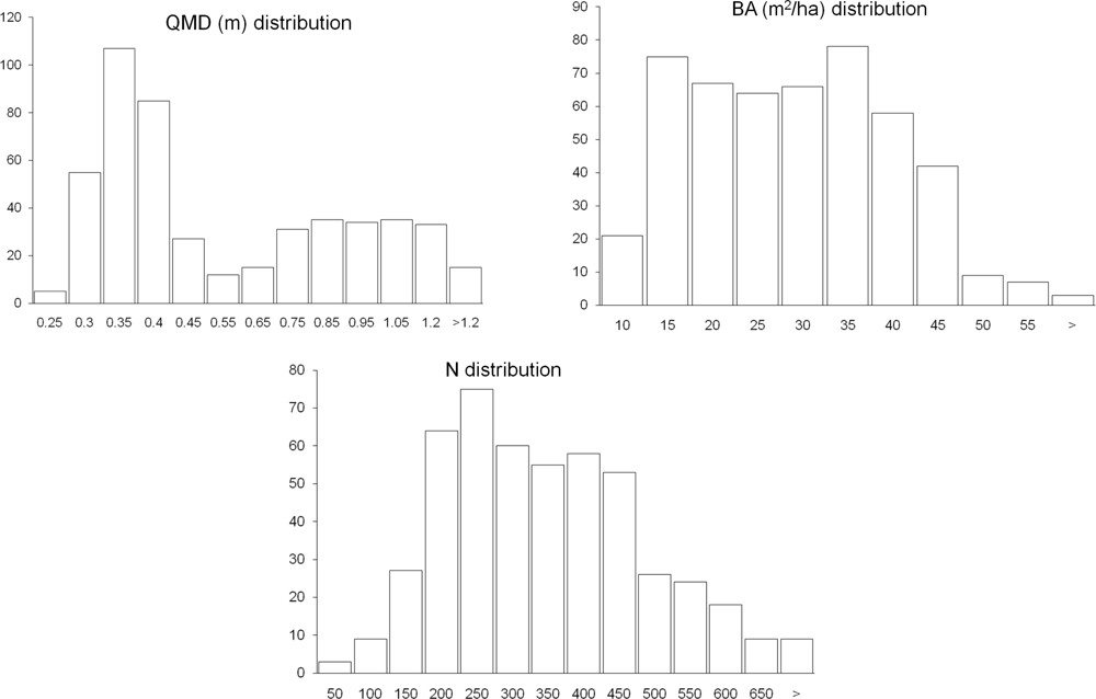
- To model the relation between structural parameters (quadratic mean diameter, basal area, and number of stems per hectare) measured via field sampling and a set of spectral and spatial variables derived from HSR multispectral and panchromatic imagery.
- To test and verify the ability of Classification and Regression Trees (CART) as the statistical technique for modeling structural parameters.
- To identify the image derived variables with the greatest informative capacity in the modeling of structural parameters, assessing in particular the inclusion of image textural metrics in the models.
2. Background
2.1. High Spatial Resolution (HSR) Imagery
2.2. HSR Related to Forest Structure
2.3. Status in the Use of Remote Sensing for Estimation of Forest Structure in Spain
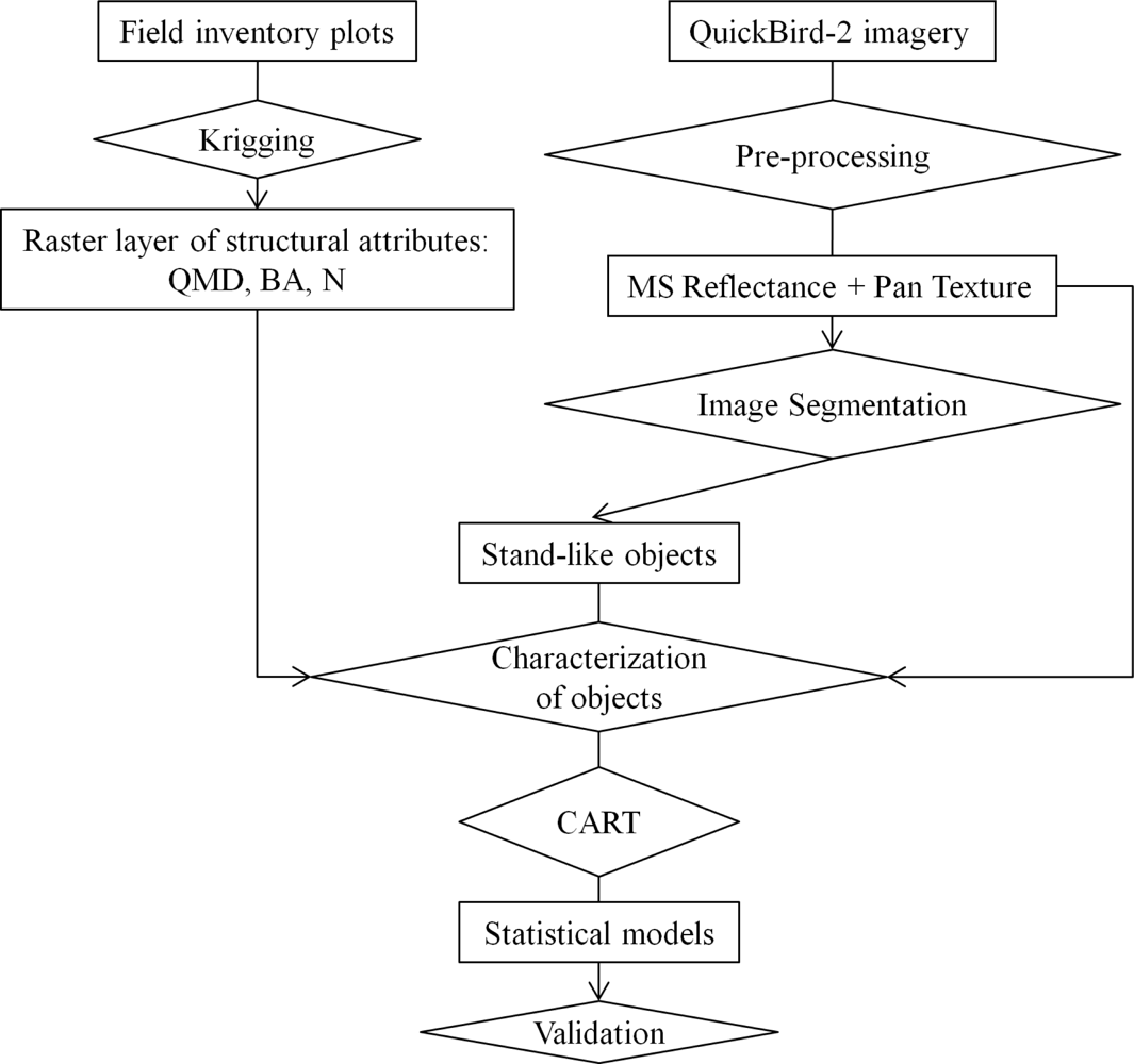
3. Methods
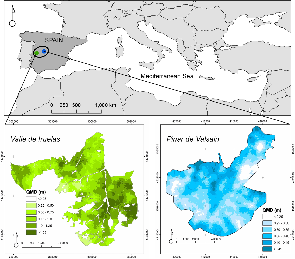
3.1. Study Area and Field Data
3.2. HSR Imagery
3.3. Image Segmentation
3.4. Image Texture Metrics
3.5. Decision Tree
3.6. Applied Decision Tree
4. Results
4.1. Stand-Like Areas Produced by Segmentation of the QuickBird-2 Imagery
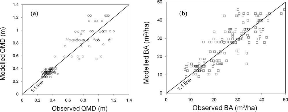
4.2. Regression Trees
5. Discussion
6. Conclusions
Acknowledgments
References
- European Forest Institute, Mediterranean Regional Office, A Mediterranean Forest Research Agenda-MFRA 2010–2020; EFIMED: Barcelona, Spain, 2009.
- Chirici, G.; Barbati, A.; Corona, P.; Marchetti, M.; Travaglini, D.; Maselli, F.; Bertini, R. Non-parametric and parametric methods using satellite images for estimating growing stock volume in alpine and Mediterranean forest ecosystems. Remote Sens. Environ 2008, 112, 2686–2700. [Google Scholar] [Green Version]
- Bravo, F.; Montero, G. High-grading effects on Scots pine volume and basal area in pure stands in northern Spain. Ann. For. Sci 2003, 60, 11–18. [Google Scholar]
- Bellassen, V.; Maire, G.; Dhote, J.F.; Ciais, P.; Viovy, N. Modelling forest management within a global vegetation model-Part 2: Model validation from a tree to a continental scale. Ecol. Model 2011, 222, 57–75. [Google Scholar]
- McRoberts, R.E.; Tomppo, E.O. Remote sensing support for national forests inventories. Remote Sens. Environ 2007, 110, 412–419. [Google Scholar]
- Falkowski, M.J.; Wulder, M.A.; White, J.C.; Gillis, M.D. Supporting large-area, sample-based forest inventories with very high spatial resolution satellite imagery. Prog. Phys. Geog 2009, 33, 403–423. [Google Scholar]
- Wulder, M.A. Optical remote sensing techniques for the assessment of forest inventory and biophysical parameters. Prog. Phys. Geog 1998, 22, 449–476. [Google Scholar]
- Wulder, M.A.; White, J.C.; Han, T.; Coops, N.C.; Cardille, J.A.; Holland, T.; Grills, D. Monitoring Canada forests. Part 2: National forest fragmentation and pattern. Can. J. Remote Sens 2008, 34, 563–584. [Google Scholar]
- Wulder, M.A.; Hall, R.J.; Coops, N.C.; Franklin, S.E. High spatial resolution remotely sensed data for ecosystem characterization. Bioscience 2004, 54, 511–521. [Google Scholar]
- Andersson, K.; Evans, T.P.; Richards, K.R. National forest carbon inventories: Policy needs and assessment capacity. Climatic Change 2009, 93, 69–101. [Google Scholar]
- Cohen, W.; Goward, S. Landsat’s role in ecological applications of remote sensing. BioScience 2004, 54, 535–545. [Google Scholar]
- Wulder, M.A.; White, J.C.; Goward, S.N.; Masek, J.G.; Irons, J.R.; Herold, M.; Cohen, W.B.; Loveland, T.R.; Woodcock, C.E. Landsat continuity: Issues and opportunities for land cover monitoring. Remote Sens. Environ 2008, 112, 955–969. [Google Scholar]
- Kayitakire, F.; Hamel, C.; Defourny, P. Retrieving forest structure variables based on image texture analysis and IKONOS-2 imagery. Remote Sens. Environ 2006, 102, 390–401. [Google Scholar]
- Colombo, R.; Bellingeri, D.; Fasolini, D.; Marino, C.M. Retrieval of leaf area index in different vegetation types using high resolution satellite data. Remote Sens. Environ 2003, 83, 120–131. [Google Scholar]
- Ouma, Y.O.; Ngigi, T.G.; Tateishi, R. On the optimization and selection of wavelet texture for feature extraction from high resolution satellite imagery with application towards urban tree delineation. Int. J. Remote Sens 2006, 27, 73–104. [Google Scholar]
- Song, C.; Dickinson, M.B.; Su, L.; Zhang, S.; Yaussey, D. Estimating average tree crown size using spatial information from IKONOS and QuickBird images: Across-sensor and across-site comparisons. Remote Sens. Environ 2010, 114, 1099–1107. [Google Scholar]
- Lu, D.; Mausel, P.; Brondizio, E.; Moran, E. Above-Ground Biomass estimation of Successional and Mature Forests Using TM Images in the Amazon Basin. Proceedings of Symposium on Geospatial Theory, Processing and Applications, Otawa, ON, Canada, 9–12 July 2002.
- Ozdemir, I. Estimating stem volume by tree crown area and tree shadow area extracted from pan-sharpened QuickBird imagery in open Crimean juniper forests. Int. J. Remote Sens 2008, 29, 5643–5655. [Google Scholar]
- Pu, R.; Landry, S.; Yu, Q. Object-based urban detailed land cover classification with high spatial resolution IKONOS imagery. Int. J. Remote Sens 2011, 32, 3285–3308. [Google Scholar]
- Wulder, M.A.; Ortlepp, S.M.; White, J.C.; Coops, N.C. Impact of sun-surface sensor geometry upon multitemporal high spatial resolution satellite imagery. Can. J. Remote Sens 2008, 34, 455–461. [Google Scholar]
- Lefsky, M.A.; Cohen, W.B.; Acker, S.A.; Parker, G.G.; Spies, T.A.; Harding, D. Lidar remote sensing of the canopy structure and biophysical properties of Douglas-fir Western Hemlock forests. Remote Sens. Environ 1999, 70, 339–361. [Google Scholar]
- Lim, K.; Treitz, P.; Baldwin, K.; Morrison, I.; Green, J. Lidar remote sensing of biophysical properties of tolerant northern hardwood forests. Can. J. Remote Sens 2003, 29, 658–678. [Google Scholar]
- Riaño, D.; Chuvieco, E.; Condés, S.; González-Matesanz, J.; Ustin, S.L. Generation of crown bulk density for Pinus sylvestris L. from lidar. Remote Sens. Environ 2004, 92, 345–352. [Google Scholar]
- Zhao, K.; Popescu, S.; Meng, X.; Pang, Y.; Agca, M. Characterizing forest canopy structure with lidar composite metrics and machine learning. Remote Sens. Environ 2011, 115, 1978–1996. [Google Scholar]
- Wulder, M.A.; White, J.C.; Hay, G.J.; Castilla, G. Towards automated segmentation of forest inventory polygons on high spatial resolution satellite imagery. Forest. Chron 2008, 84, 221–230. [Google Scholar]
- Gougeon, F.A.; Leckie, D.G. The individual tree crown approach applied to IKONOS images of a coniferous plantation area. Photogram. Eng. Remote Sensing 2006, 72, 1287–1297. [Google Scholar]
- Hirata, Y. Estimation of stand attributes in Cryptomeria japonica and Chamaecyparis obtusa stands using QuickBird panchromatic data. J. Forest Res 2008, 13, 147–154. [Google Scholar]
- Leboeuf, A.; Beaudoin, A.; Fournier, R.A.; Guindon, L.; Luther, J.E.; Lambert, M.C. A shadow fraction method for mapping biomass of northern boreal black spruce forests using QuickBird imagery. Remote Sens. Environ 2007, 110, 488–500. [Google Scholar]
- Franklin, S.E.; Wulder, M.A.; Gerylo, G.R. Texture analysis of IKONOS panchromatic data for Douglas-fir forest age class separability in British Columbia. Int. J. Remote Sens 2001, 22, 2627–2632. [Google Scholar]
- Ozdemir, I.; Norton, D.A.; Ozkan, U.Y.; Mert, A.; Senturk, O. Estimation of tree size diversity using object oriented texture analysis and ASTER imagery. Sensors 2008, 8, 4709–4724. [Google Scholar]
- Song, C. Estimating tree crown size with spatial information of high resolution optical remotely sensed imagery. Int. J. Remote Sens 2007, 28, 3305–3322. [Google Scholar]
- Feng, Y.; Li, Z.; Tokola, T. Estimation of stand mean crown diameter from high-spatial-resolution imagery based on a geostatistical method. Int. J. Remote Sens 2010, 31, 363–378. [Google Scholar]
- Merino de Miguel, S.; Solana Gutiérrez, J.; González Alonso, F. Análisis de la estructura espacial de las masas de Pinus pinaster Aiton de la Comunidad de Madrid mediante imágenes de alta resolución espacial. Forest Syst 2010, 19, 18–35. [Google Scholar]
- Duncanson, L.I.; Niemann, K.O.; Wulder, M.A. Integration of GLAS and Landsat TM data for aboveground biomass estimation. Can. J. Remote Sens 2010, 36, 129–141. [Google Scholar]
- Greenberg, J.A.; Dobrowsky, S.Z.; Ustin, S.L. Shadow allometry: Estimating tree structural parameters using hyperspatial image analysis. Remote Sens. Environ 2005, 97, 15–25. [Google Scholar]
- Hyde, P.; Dubayah, R.; Walker, W.; Blair, B.; Hofton, M.; Hunsaker, C. Mapping forest structure for wildlife habitat analysis using multi-sensor (LiDAR, SAR/InSAR, ETM+, Quickbird) synergy. Remote Sens. Environ 2006, 102, 63–73. [Google Scholar]
- Chubey, M.S.; Franklin, S.E.; Wulder, M.A. Object-based analysis of IKONOS-2 imagery for extraction of forest inventory parameters. Photogramm. Eng. Remote Sensing 2006, 72, 383–394. [Google Scholar]
- Proisy, Ch.; Couteron, P.; Fromard, F. Predicting and mapping mangrove biomass from canopy grain analysis using Fourier-based textural ordination of IKONOS images. Remote Sens. Environ 2007, 109, 379–392. [Google Scholar]
- Palace, M.; Keller, M.; Asner, G.P.; Hagen, S.; Braswell, B. Amazon forest structure from IKONOS satellite data and the automated characterization of forest canopy properties. Biotropica 2008, 40, 141–150. [Google Scholar]
- Mora, B.; Wulder, M.A.; White, J.C. Segment-constrained regression tree estimation of forest stand height from very high spatial resolution panchromatic imagery over a boreal environment. Remote Sens. Environ 2010, 114, 2474–2484. [Google Scholar]
- Arozarena, A. El Plan Nacional de Observación del territorio en España como sistema básico de información Medio Ambiental. Congreso Nacional del Medio Ambiente, Cumbre del Desarrollo Sostenible, Madrid, Spain, 1–5 December 2008.
- Villa, G.; Arozarena, A.; Peces, J.J.; Domenech, E. Plan nacional de teledetección: estado actual y perspectivas futuras. Proceedings of Teledetección: agua y desarrollo sostenible. XIII Congreso de la Asociación Española de Teledetección, Calatayud, Spain, 23–26 September 2009; pp. 521–524.
- IGN, Plan Nacional de Teledetección (PNT); Versión 2.3; Ministerio de Fomento, Gobierno de España: Madrid, Spain, 2009.
- Vázquez de la Cueva, A. Structural attributes of three forest types in central Spain and Landsat ETM+ information evaluated with redundancy analysis. Int. J. Remote Sens 2008, 29, 5657–5676. [Google Scholar]
- Pascual, C.; García Abril, A.; García Montero, L.G.; Martín Fernández, S.; Cohen, W.B. Object-based semi-automatic approach for forest structure characterization using lidar data in heterogeneous Pinus sylvestris stands. Forest Ecol. Manag 2008, 255, 3677–3685. [Google Scholar]
- Montes, F.; Sánchez, M.; Río, M.; Cañellas, I. Using historic management records to characterize the effects of management on the structural diversity of forests. Forest Ecol. Manag 2004, 207, 279–293. [Google Scholar]
- Bravo, F.; Río, M.; Pando, V.; San Martín, R.; Montero, G.; Ordoñez, C.; Cañellas, I. El diseño de las parcelas del inventario forestal nacional y la estimación de variables dasómetricas. In El Inventario Forestal Nacional, Elemento Clave para la Gestión Forestal Sostenible; Bravo, F., Rio, M., Peso, C., Eds.; Fundación General de la Universidad de Valladolid: Valladolid, Spain, 2002; pp. 19–35. [Google Scholar]
- Curtis, R.O.; Marshall, D.D. Why quadratic mean diameter? West. J. Appl. For 2000, 15, 137–139. [Google Scholar]
- Chica-Olmo, M. La geoestadística como herramienta de análisis en la gestión forestal. Cuad. Soc. Esp. Cienc. For 2005, 19, 47–55. [Google Scholar]
- Curran, P.J.; Atkinson, P.M. Geostatistics and remote sensing. Prog. Phys. Geog 1998, 22, 61–78. [Google Scholar]
- Clark, I. Practical Geostatistics; Geostokos Limited: Scotland, UK, 2001. Available online: http://w3eos.whoi.edu/12.747/resources/pract_geostat/pg1979_latex.pdf (accessed on 17 May 2011).
- DigitalGlobe. QuickBird Imagery Products FAQ; Houston, TX, USA, 2005. Available online: http://www.satimagingcorp.com/satellite-sensors/quickbird_imagery_products.pdf (accessed on 17 October 2011).
- Chavez, P.S. Image-based atmospheric corrections—Revisited and improved. Photogramm. Eng. Remote Sensing 1996, 62, 1025–1036. [Google Scholar]
- Chavez, P. An improved dark object subtraction technique for atmospheric scattering correction of multispectral data. Remote Sens. Environ 1988, 24, 459–479. [Google Scholar]
- Devereux, B.J.; Amable, G.S.; Costa Posada, C. An efficient image segmentation algorithm for landscape analysis. Int. J. Appl. Earth Obs. Geoinf 2004, 6, 47–61. [Google Scholar]
- Hay, G.J.; Castilla, G.; Wulder, M.A.; Ruiz, J.R. An automated object-based approach for the multiscale image segmentation of forest scenes. Int. J. Appl. Earth Obs. Geoinf 2005, 7, 339–359. [Google Scholar]
- Baatz, M.; Schäpe, M. Multiresolution segmentation—An optimization approach for high quality multi-scale image segmentation. In Angewandte Geographische Informations-Verarbeitung XII; Strobl, J., Blaschke, T., Griesebner, G., Eds.; Wichmann Verlag: Karlsruhe, Germany, 2000; pp. 12–23. [Google Scholar]
- Definiens, Definiens Professional 5 User Guide; Definiens: Munich, Germany, 2006.
- Salvador, R.; Pons, X. On the applicability of Landsat TM images to Mediterranean forest inventories. Forest Ecol. Manag 1998, 104, 193–208. [Google Scholar]
- Haralick, R.M.; Bryant, W.F. Documentation of Procedures for Textural/Spatial Pattern Recognition Techniques; Technical Report 278-1; Remote Sensing Laboratory, University of Kansas: Lawrence, KS, USA, 1976. [Google Scholar]
- Wulder, M.A.; LeDrew, E.F.; Franklin, S.E.; Lavigne, M.B. Aerial texture information in the estimation of northern deciduous and mixed wood forest leaf area index (LAI). Remote Sens. Environ 1998, 64, 64–76. [Google Scholar]
- Lu, D. The potential and challenge of remote sensing-based biomass estimation. Int. J. Remote Sens 2006, 27, 1297–1328. [Google Scholar]
- Franklin, S.E.; Hall, R.J.; Moskal, L.M.; Maudie, A.J.; Lavigne, M.B. Incorporating texture into classification of forest species composition from airborne multispectral images. Int. J. Remote Sens 2000, 21, 61–79. [Google Scholar]
- Couteron, P.; Pelissier, R.; Nicolini, E.A.; Paget, D. Predicting tropical forest stand structure parameters from Fourier transform of very high-resolution remotely sensed canopy images. J. App. Ecol 2005, 42, 1121–1128. [Google Scholar]
- Lu, D.; Batistella, M. Exploring TM image texture and its relationships with biomass estimation in Rondonia, Brazilian Amazon. Acta Amazonica 2005, 35, 249–257. [Google Scholar]
- Haralick, R.M.; Shanmugan, K.; Dinstein, I. Texture features for image classification. IEEE T. Syst. Man Cyb 1973, 3, 610–621. [Google Scholar]
- Caridade, C.M.R.; Marca, A.R.S.; Mendonca, T. The use of texture for image classification of black & white air photographs. Int. J. Remote Sens 2008, 29, 593–607. [Google Scholar]
- Hall-Beyer, M. GLCM Tutorial Home Page. 2007. Available online: http://www.fp.ucalgary.ca/mhallbey/tutorial.htm (accessed on 13 October 2011).
- Ahearn, S.C. Combining Laplacian images of different spatial frequencies (scales): Implications for remote sensing analysis. IEEE Trans. Geosci. Remote Sens 1988, 26, 826–831. [Google Scholar]
- Ferro, C.; Warner, T. Scale and texture in digital image classification. Photogramm. Eng. Remote Sensing 2002, 68, 51–63. [Google Scholar]
- Johansen, K.; Coops, N.C.; Gergel, S.E.; Stange, Y. Application of high spatial resolution satellite imagery for riparian and forest ecosystem classification. Remote Sens. Environ 2007, 110, 29–44. [Google Scholar]
- Nijland, W.; Addink, E.A.; de Jong, S.M.; Van der Meer, F.D. Optimizing spatial image support for quantitative mapping of natural vegetation. Remote Sens. Environ 2009, 113, 771–780. [Google Scholar]
- Montes, F.; Rubio, A.; Barbeito, I.; Cañellas, I. Characterization of the spatial structure of the canopy in Pinus sylvestris L. stands in Central Spain from hemispherical photographs. Forest Ecol. Manag 2008, 255, 580–590. [Google Scholar]
- Pal, M.; Mather, P.M. An assessment of the effectiveness of decision tree methods for land cover classification. Remote Sens. Environ 2003, 86, 554–565. [Google Scholar]
- Baccini, A.; Laporte, N.; Goetz, S.J.; Sun, M.; Dong, H. A first map of tropical Africa’s above-ground biomass derived from satellite imagery. Environ. Res. Let 2008, 3, 045011. [Google Scholar]
- Breiman, L.; Friedman, J.H.; Olshen, R.A.; Stone, C.J. Classification and Regression Trees; Chapman and Hall/CRC: Boca Raton, FL, USA, 1984; p. 358. [Google Scholar]
- Brown de Colstoun, E.C.; Story, M.H.; Thompson, C.; Commisso, K.; Smith, T.G.; Irons, J.R. National Park vegetation mapping using multitemporal Landsat 7 data and a decision tree classifier. Remote Sens. Environ 2003, 85, 316–327. [Google Scholar]
- Mcdermid, G.J.; Smith, I.U. Mapping the distribution of whitebark pine (Pinus albicaulis) in Waterton Lakes National Park using logistic regression and classification tree analysis. Can. J. Remote Sens 2008, 34, 356–366. [Google Scholar]
- Ke, Y.; Quackenbush, L.J.; Im, J. Synergistic use of QuickBird multispectral imagery and LIDAR data for object-based forest species classification. Remote Sens. Environ 2010, 114, 1141–1154. [Google Scholar]
- Andrew, M.E.; Ustin, S.L. Habitat Suitability Modeling of an invasive plant with advanced remote sensing data. Divers. Distrib 2009, 15, 627–640. [Google Scholar]
- Im, J.; Jensen, J.R. A change detection model based on neighborhood correlation image analysis and decision tree classification. Remote Sens. Environ 2005, 99, 326–340. [Google Scholar]
- Lozano, F.J.; Suárez-Seoane, S.; Kelly, M.; Luis, E. A multi-scale approach for modeling fire occurrence probability using satellite data and classification trees: A case study in a mountainous Mediterranean region. Remote Sens. Environ 2008, 112, 708–719. [Google Scholar]
- Falkowski, M.J.; Evans, J.; Martinuzzi, S.; Gessler., P.E.; Hudak, A.T. Characterizing forest succession with lidar data: an evaluation for the Inland Northwest, USA. Remote Sens. Environ 2009, 113, 946–956. [Google Scholar]
- Goetz, S.J.; Wright, R.K.; Smith, A.J.; Zinecker, E.; Schaub, E. IKONOS imagery for resource management: tree cover, impervious surfaces, and riparian buffer analyses in the mid-Atlantic region. Remote Sens. Environ 2003, 88, 195–208. [Google Scholar]
- Biondini, M.E.; Mielke, P.W., Jr.; Berry, K.J. Data-dependent permutation techniques for the analysis of ecological data. Vegetatio 1988, 75, 161–168. [Google Scholar]
- Mielke, P.W., Jr.; Berry, K.J. Permutation Methods: A Distance Function Approach; Springer Series in Statistics; Springer: New York, NY, USA, 2001. [Google Scholar]
- Foody, G.M.; Cutler, M.E.; McMorrow, J.; Pelz, D.; Tangki, H.; Boyd, D.S.; Douglas, I. Mapping the biomass of Bornean tropical rain forest from remotely sensed data. Global Ecol. Biogeogr 2001, 10, 379–387. [Google Scholar]
- Wulder, M.A.; Niemann, K.O.; Goodenough, D.G. Error reduction methods for local maximum filtering. Can. J. Remote Sens 2002, 28, 667–671. [Google Scholar]
- Bernués, D. La gestión forestal sostenible en Aragon. Foresta 2008, 43, 104–107. [Google Scholar]
- MMA, Anuario de Estadística Forestal 2008; Ministerio de Medio Ambiente y Medio Rural y Marino: Madrid, Spain, 2008; p. 96.
- Wulder, M.A.; Kurz, W.A.; Gillis, M. National level forest monitoring and modeling in Canada. Prog. Phys. Plan 2004, 61, 365–381. [Google Scholar]
- Culvenor, D.S. Extracting individual tree information: A survey of techniques for high spatial resolution imagery. In Remote Sensing of Forest Environments: Concepts and Case Studies; Wulder, M.A., Franklin, S.E., Eds.; Kluwer Academic Publishers: Boston, MA, USA, 2003; pp. 255–277. [Google Scholar]
- Aguilar, M.A.; Agüera, F.; Aguilar, F.J.; Carvajal, F. Geometric accuracy assessment of the orthorectification process from very high resolution satellite imagery for common agricultural policy purposes. Int. J. Remote Sens 2008, 29, 7181–7197. [Google Scholar]
- Bruniquel-Pinel, V.; Gastellu-Etchegorry, J.P. Sensitivity of texture of high resolution images of forest to biophysical and acquisition parameters. Remote Sens. Environ 1998, 65, 61–85. [Google Scholar]
- Maselli, F. Monitoring forest conditions in a protected Mediterranean coastal area by the analysis of multiyear NDVI data. Remote Sens. Environ 2004, 89, 423–433. [Google Scholar]
- Leckie, D.G.; Gougeon, F.A.; Walsworth, N.; Paradine, D. Stand delineation and composition estimation using semi-automated individual tree crown analysis. Remote Sens. Environ 2003, 85, 355–369. [Google Scholar]
- Lamonaca, A.; Corona, P.; Barbati, A. Exploring forest structural complexity by multi-scale segmentation of VHR imagery. Remote Sens. Environ 2008, 112, 2839–2849. [Google Scholar] [Green Version]


| Study | Attribute | Environment | Sensor | Statistical Analysis | Best Result |
|---|---|---|---|---|---|
| Location | Data (spa. res., m) | Parameter | |||
| [29] | Age class | Sooke River watershed | IKONOS | ANOVA | Homogeneity in large window sizes performs better than variance |
| British Columbia (Canada) | Pan (0.82) | Texture measures | |||
| [26] | Stem density | Conifer plantation | IKONOS | Delineation | 83% accuracy |
| Ontario (Canada) | Pan (0.87) | Tree crown delineation | |||
| [35] | Diameter | Lake Tanoe Basin | IKONOS | Linear regression | R = 0.67 |
| Crown area | California (USA) | Pan-sharpened (1) | Crown shadow | R = 0.77 | |
| R = 0.87 | |||||
| Stem density | |||||
| [13] | Circumference | Even aged Norway spruce forest | IKONOS-2 | Linear regression | R2 = 0.82 |
| Height | R2 = 0.76 | ||||
| Stand density | Hautes-Fagnes (Belgium) | Pan (0.87) | GLCM textural metrics | R2 = 0.82 | |
| Age | R2 = 0.81 | ||||
| Basal area | R2 = 0.35 | ||||
| [36] | Maximum height | Conifers | QuickBird | Linear regression | R2=0.66 |
| Sierra Nevada mountains California (USA) | MS (2) | Reflectance | |||
| [37] | Height | Mature forest in the foothills of the Rocky Mountains | IKONOS | Decision tree | Accuracy 49% |
| Age | Accuracy 57% | ||||
| Crown closure | Accuracy 85% | ||||
| Alberta (Canada) | MS (4) and Pan (1) | Reflectance and texture | |||
| [28] | Biomass | Boreal spruce forest | QuickBird | Linear regression | R2 = 0.87 |
| Canada | Pansharpened (0.6) | Shadow fraction | |||
| [31] | Mean crown size | Conifer and hardwood | IKONOS | Linear regression | R2 = 0.73 |
| North Carolina (USA) | Pan (not reported) | Variogram Image variance ratio | |||
| RMSE = 0.10 | |||||
| [38] | Biomass | Mangrove | IKONOS | Linear regression | R2 = 0.92 |
| French Guiana | NIR (4) Pan (1) | Fourier textural ordination indices | |||
| [27] | Stand density | Coniferous plantations in slopes | QuickBird | Modeling-allometry | R = 0.82 density |
| Shikoku Iskland (Japan) | Pan (0.61) | Reflectance | |||
| Stand volume | R = 0.78 volume | ||||
| [39] | Crown width | Tropical forest | IKONOS | Allometric equations | Crown within 3% of field measures |
| Brazil | Pan (1.00) | Local extreme filter | |||
| Tree diameter | |||||
| Stem frequency | |||||
| [18] | Volume | Open Juniperus forest | QuickBird | Linear regression | R2 = 0.67 |
| Turkey | Pansharpened (0.61) | Shadow area | |||
| Crown area | R2 = 0.51 | ||||
| [32] | Mean crown size | Pine and poplar plant. | QuickBird | Variogram | Error: 2.52–42% |
| Beijing and Shanxi, (China) | Pan (0.61–0.67) | Reflectance | |||
| [16] | Mean crown size | Hardwoods | IKONOS and QuickBird | Linear regression | R2 = 0.60 regression CD∼variance ratio (RMSE = 0.82) |
| Ohio and North Carolina (USA) | Pan (1) Pan (0.73) | Image variance ratio | |||
| R2 = 0.74 across site comparison | |||||
| R2 = 0.52 across sensors | |||||
| [40] | Mean stand height | Boreal forest | QuickBird | Regression tree | R2 = 0.53 |
| Yukon, Canada | Pan (0.68) | Reflectance | |||
| RMSE=2.84 m | |||||
| QuickBird-2 Imagery | ||
|---|---|---|
| Spatial resolution | Multispectral | 2.4 m |
| Panchromatic | 0.68 m | |
| Bands | Blue | 0.45–0.52 μm |
| Green | 0.52–0.60 μm | |
| Red | 0.63–0.69 μm | |
| NIR | 0.76–0.90 μm | |
| Pan | 0.45–0.90 μm | |
| Valsaín | Iruelas | |
| Date (dd/mm/yyyy) | 19/05/2004 | 05/08/2005 |
| Sun elevation (°) | 58.4 | 72.0 |
| Predictor Variable | Description |
|---|---|
| Reflectance | |
| B1 (Blue) | Reflectance band 1 |
| B2 (Green) | Reflectance band 2 |
| B3 (Red) | Reflectance band 3 |
| B4 (NIR) | Reflectance band 4 |
| Textural | |
| H_S | Homogeneity Small window |
| Con_S | Contrast Small window |
| E_S | Entropy Small window |
| H_M | Homogeneity Medium window |
| Con_M | Contrast Medium window |
| E_M | Entropy Medium window |
| H_L | Homogeneity Large window |
| Con_L | Contrast Large window |
| E_L | Entropy Large window |
| Topographic | |
| Aspect | Orientation |
| QMD(m) | BA(m2/ha) | N(n/ha) | Aspect (θ°) | |
|---|---|---|---|---|
| Mean | 0.5715 | 26.5344 | 323.2064 | 168.5636 |
| Standard Error | 0.0138 | 0.5044 | 6.4277 | 4.3050 |
| Median | 0.3918 | 26.5148 | 306.461 | 155.2855 |
| Standard Deviation | 0.3062 | 11.1671 | 142.2839 | 95.2968 |
| Kurtosis | −0.7460 | −0.6941 | 0.1987 | −1.2352 |
| Skewness | 0.7943 | 0.2266 | 0.6035 | 0.1926 |
| Range | 1.2407 | 53.8552 | 805.0587 | 337.2344 |
| Minimum | 0.2148 | 5.8128 | 39.1273 | 10.1746 |
| Maximum | 1.4555 | 59.6681 | 844.186 | 347.4090 |
| Samples | Stand-Like Segments |
|---|---|
| Total | 490 |
| Calibration | 327 |
| Validation | 163 |
| Structural Parameter | Validation | Fitting | |||
|---|---|---|---|---|---|
| RMSE | % Average Error | R2 | Rho | p-value | |
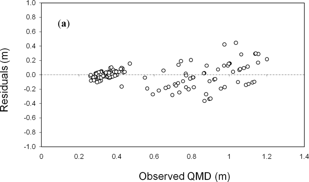
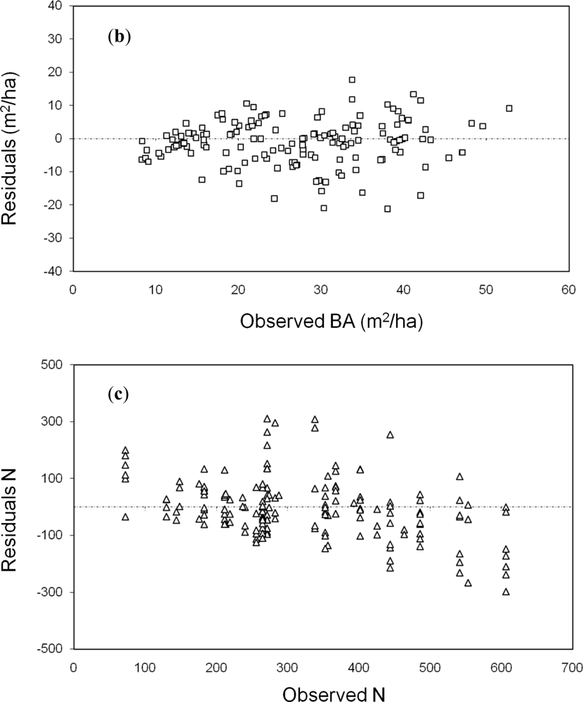
| QMD | 0.13 | 17 | 0.80 | 0.89 | 1.81 e-59 |
| BA | 5.79 | 22 | 0.70 | 0.85 | 7.08 e-47 |
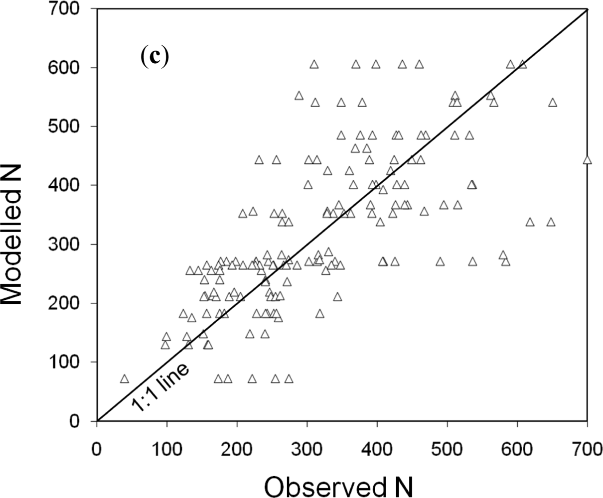
| N | 98.86 | 31 | 0.46 | 0.71 | 1.80 e-26 |
| Structural Parameter | Relevant Predictors | Terminal Nodes |
|---|---|---|
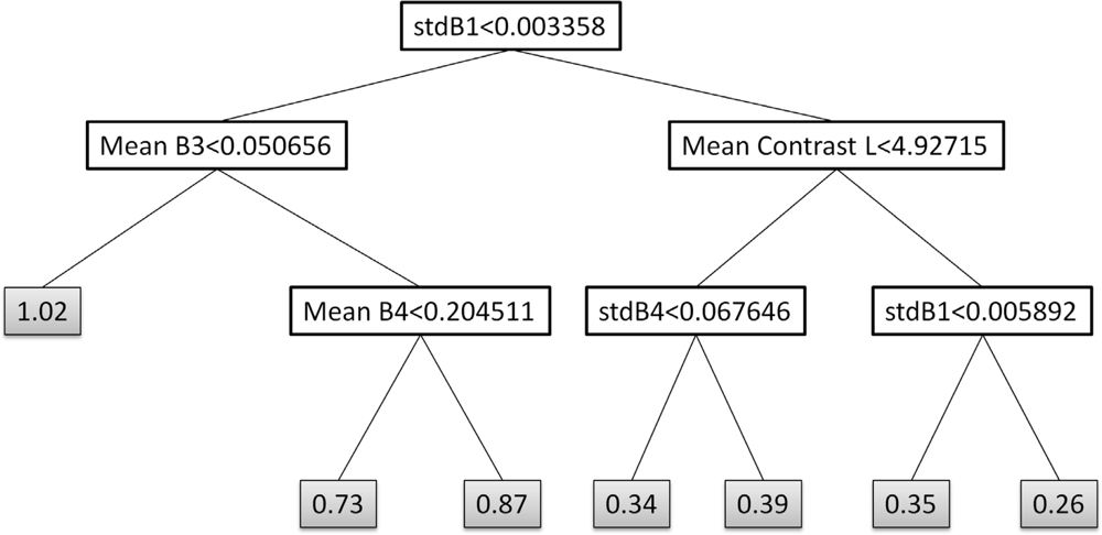
| QMD | Stdev B1 | 7 |
| Mean B3 | ||
| Mean Contrast Larger window | ||
| Mean B4 | ||
| Standard deviation B4 | ||
| BA | Stdev B1 | 7 |
| Mean B3 | ||
| Mean B1 | ||
| Standard deviation B2 | ||
| Mean Entropy Small window | ||
| N | Stdev B1 | 8 |
| Mean B1 | ||
| Standard deviation B4 | ||
| Mean Entropy Medium window | ||
| Mean B2 | ||
| Mean B3 | ||
Share and Cite
Gómez, C.; Wulder, M.A.; Montes, F.; Delgado, J.A. Modeling Forest Structural Parameters in the Mediterranean Pines of Central Spain using QuickBird-2 Imagery and Classification and Regression Tree Analysis (CART). Remote Sens. 2012, 4, 135-159. https://doi.org/10.3390/rs4010135
Gómez C, Wulder MA, Montes F, Delgado JA. Modeling Forest Structural Parameters in the Mediterranean Pines of Central Spain using QuickBird-2 Imagery and Classification and Regression Tree Analysis (CART). Remote Sensing. 2012; 4(1):135-159. https://doi.org/10.3390/rs4010135
Chicago/Turabian StyleGómez, Cristina, Michael A. Wulder, Fernando Montes, and José A. Delgado. 2012. "Modeling Forest Structural Parameters in the Mediterranean Pines of Central Spain using QuickBird-2 Imagery and Classification and Regression Tree Analysis (CART)" Remote Sensing 4, no. 1: 135-159. https://doi.org/10.3390/rs4010135