Object-Based Image Analysis of Downed Logs in Disturbed Forested Landscapes Using Lidar


Abstract
:1. Introduction
1.1. Remote Sensing and Lidar in Forest Science
1.2. Object-Based Image Analysis and Forest Science

| Remotely Sensed Input Data | Location | Application | Reference |
|---|---|---|---|
| Landsat ETM+ | British Columbia, Canada | Land cover & logging scar classification | [61] |
| DAIS | Point Reyes, California. USA | Vegetation species classification | [71] |
| IKONOS | Flanders, Belgium | Forest land cover classification | [67] |
| IKONOS | Marin County, California, USA | Forest edge mapping | [72] |
| IKONOS | Western Alberta, Canada | Forest inventory mapping | [60] |
| IKONOS | British Columbia, Canada | Forest inventory mapping | [68] |
| IKONOS | North Carolina, USA | Forest type mapping | [42] |
| ADAR | China Camp State Park, California, USA | Tree mortality classification | [19,21] |
| QuickBird | Madrid, Spain | Fire fuel type mapping | [77] |
| QuickBird + Lidar (discrete, 4 return) | Central Queensland, Australia | Riparian biodiversity and wildlife habitats | [73,74] |
| CIR digital aerial photography (0.5m) | Great Smoky Mountains National Park, USA | Forest type mapping | [78] |
| Lidar (discrete, 4 returns) | Olympia, Washington, USA | Forest stand mapping | [70] |
| Lidar (discrete, 2 returns) | Central Spain | Forest inventory mapping | [75] |
| Lidar (discrete, 2 returns) | Victoria, Australia | Riparian forest mapping | [76] |
| SPOT + Lidar (discrete, 2 returns) | Garonne & Allier rivers, France | Land cover & forest age classification | [31] |
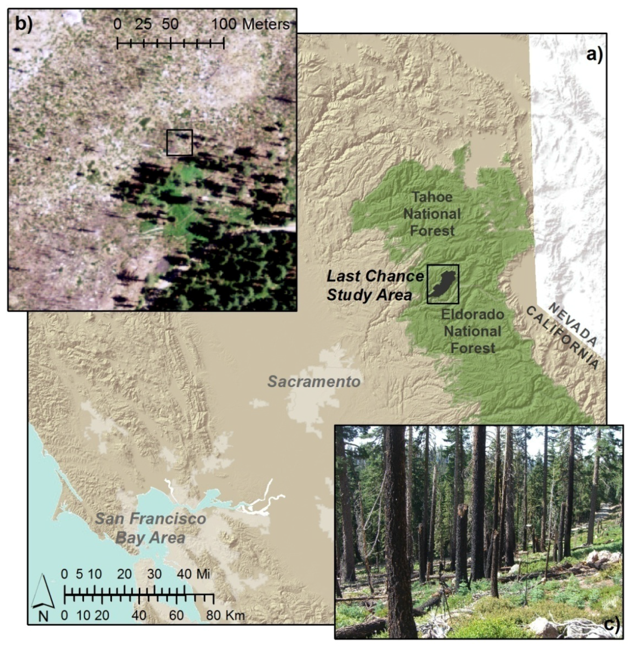
2. Study Area
3. Data
3.1. Lidar Data
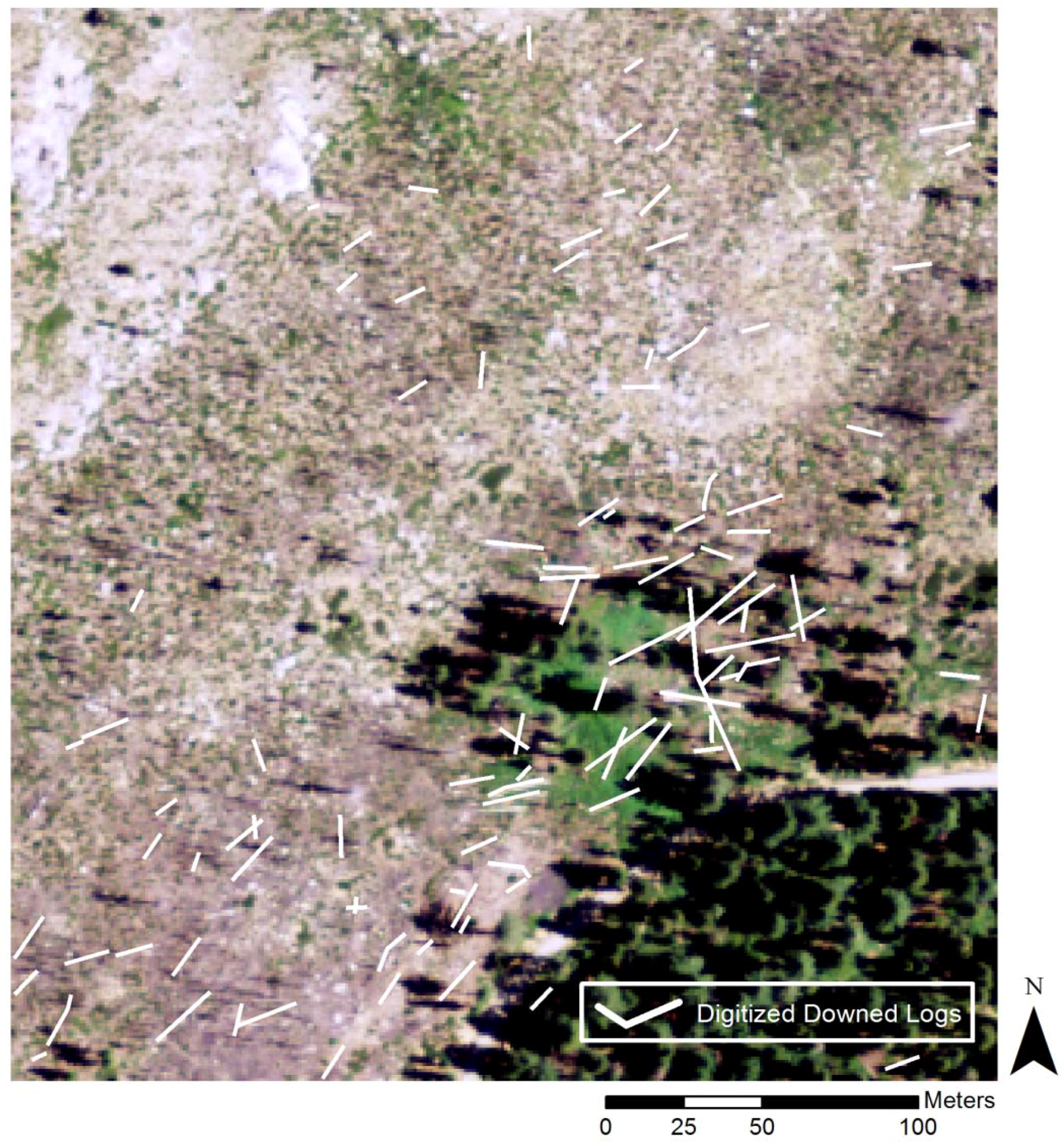
3.2. Downed Log Validation Data
4. Methods
4.1. Object-Based Image Analysis Input Layers
| Rank | Data | Post-Processing | OBIA Application |
|---|---|---|---|
| 1 | Lidar data TIN* surface | Vector thematic layer | |
| 2 | Elevation standard deviation | 3 × 3 high pass filter & boolean reclassification | Raster data layer |
| 3 | Elevation minimum | Boolean reclassification | Raster data layer |
| 4 | Total number of points | Raster data layer | |
| 5 | Total number of points | 3 × 3 low pass filter | Raster data layer |
| 6 | Total number of points | 3 × 3 median filter | Raster data layer |
| 7 | Total number of points | 3 × 3 Sobel filter | Raster data layer |
| 8 | Absolute roughness | Raster data layer | |
| 9 | Intensity | Raster data layer | |
| 10 | Point density | Raster data layer | |
| 11 | Slope | Raster data layer |
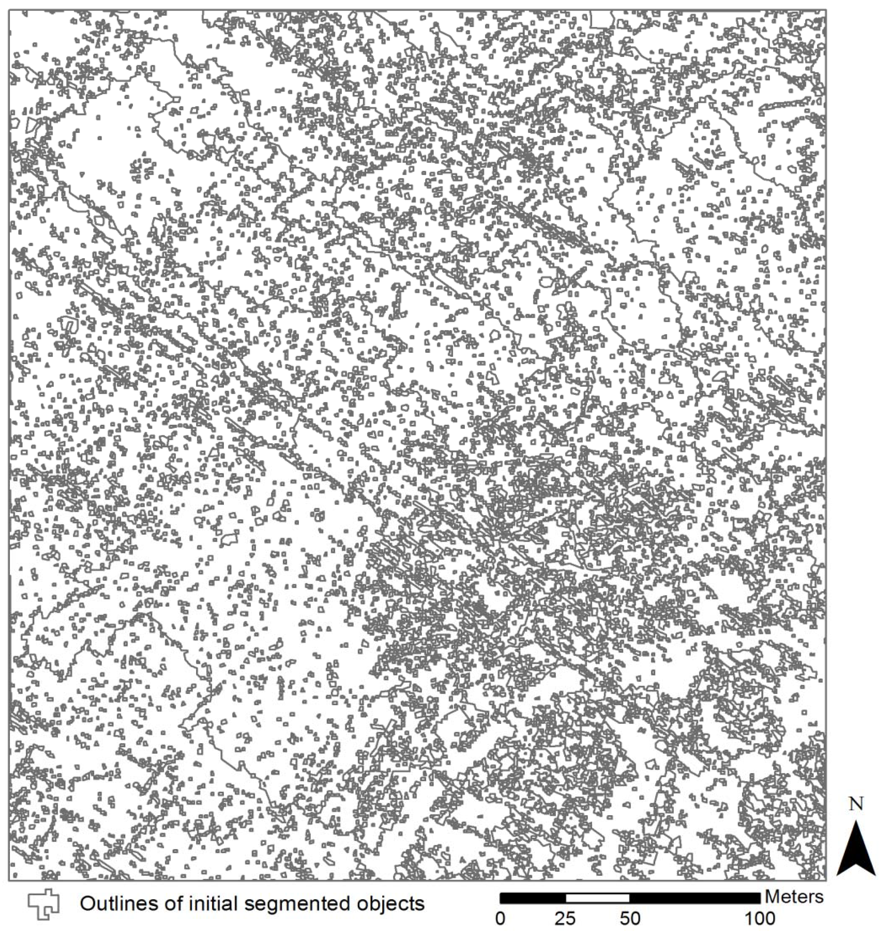
4.2. Object-Based Image Analysis
4.3. Object-Based Image Analysis Classification Accuracy Assessment
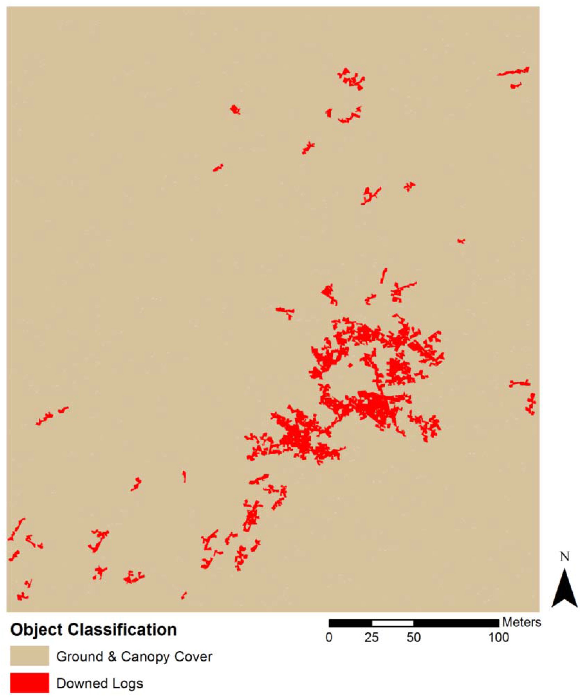
5. Results
| Class | Statistic | Data Layer | |||||||||
|---|---|---|---|---|---|---|---|---|---|---|---|
| Elevation standard deviation1 | Elevation minimum2 | Total number of points | Total number of points3 | Total number of points4 | Total number of points5 | Absolute roughness | Intensity | Point density | Slope | ||
| Downed logs | Min. | 0.34 | 0.34 | 0.50 | 0.44 | 0.24 | 3.90 | 0.05 | 99.67 | 13.16 | 8.63 |
| Max. | 1 | 0.86 | 2.61 | 2.55 | 2.35 | 13.69 | 0.19 | 153.42 | 24.32 | 25.06 | |
| Mean | 0.87 | 0.68 | 1.40 | 1.31 | 1.10 | 7.86 | 0.13 | 118.97 | 16.65 | 18.92 | |
| Ground & canopy cover | Min. | 0 | 0 | 0 | 0 | 0 | 0 | −1 | −1 | −1 | −1 |
| Max. | 1 | 1 | 13 | 11.51 | 12.80 | 68 | 0.54 | 968.42 | 60 | 55.45 | |
| Mean | 0.79 | 0.68 | 1.54 | 1.39 | 1.16 | 8.28 | 0.14 | 115.79 | 18.22 | 20 | |

6. Discussion
7. Conclusion
Acknowledgments
References
- Kueppers, L.M.; Southon, J.; Baer, P.; Harte, J. Dead wood biomass and turnover time, measured by radiocarbon, along a subalpine elevation gradient. Oecologia 2004, 141, 641–651. [Google Scholar] [CrossRef] [PubMed]
- Schiegg, K. Effects of dead wood volume and connectivity on saproxylic insect species diversity. Ecoscience 2000, 7, 290–298. [Google Scholar]
- Dixon, R.K.; Solomon, A.; Brown, S.; Houghton, R.; Trexier, M.; Wisniewski, J. Carbon pools and flux of global forest ecosystems. Science 1994, 263, 185. [Google Scholar] [CrossRef] [PubMed]
- Scott, J.H.; Burgan, R.E. Standard Fire Behavior Fuel Models: A Comprehensive Set for Use with Rothermel’s Surface Fire Spread Model; USDA Forest Service, Rocky Mountain Research Station: Fort Collins, CO, USA, 2005; p. 72.
- van Wagtendonk, J.W.; Benedict, J.M.; Sydoriak, W.M. Fuel bed characteristics of Sierra Nevada conifers. Western J. Appl. Forest. 1998, 13, 73–84. [Google Scholar]
- Janisch, J.; Harmon, M. Successional changes in live and dead wood carbon stores: Implications for net ecosystem productivity. Tree Physiol. 2002, 22, 77. [Google Scholar] [CrossRef] [PubMed]
- Pesonen, A.; Maltamo, M.; Eerikainen, K.; Packalen, P. Airborne laser scanning-based prediction of coarse woody debris volumes in a conservation area. Forest Ecol. Manage. 2008, 255, 3288–3296. [Google Scholar] [CrossRef]
- Rouvinen, S.; Kuuluvainen, T. Amount and spatial distribution of standing and downed dead trees in two areas of different fire history in a boreal Scots pine forest. Ecol. Bull. 2001, 49, 115–127. [Google Scholar]
- Bobiec, A. Living stands and dead wood in the Biaowiea forest: Suggestions for restoration management. Forest Ecol. Manage. 2002, 165, 125–140. [Google Scholar] [CrossRef]
- Christensen, M.; Hahn, K.; Mountford, E.P.; Odor, P.; Standovar, T.; Rozenbergar, D.; Diaci, J.; Wijdeven, S.; Meyer, P.; Winter, S. Dead wood in European beech (Fagus sylvatica) forest reserves. Forest Ecol. Manage. 2005, 210, 267–282. [Google Scholar] [CrossRef]
- Butler, R.; Angelstam, P.; Ekelund, P.; Schlaepfer, R. Dead wood threshold values for the three-toed woodpecker presence in boreal and sub-Alpine forest. Biol. Conserv. 2004, 119, 305–318. [Google Scholar] [CrossRef]
- Jordan, G.J.; Ducey, M.J.; Gove, J.H. Comparing line-intersect, fixed-area, and point relascope sampling for dead and downed coarse woody material in a managed northern hardwood forest. Can. J. Forest Res. 2004, 34, 1766–1775. [Google Scholar] [CrossRef]
- Pasher, J.; King, D.J. Mapping dead wood distribution in a temperate hardwood forest using high resolution airborne imagery. Forest Ecol. Manage. 2009, 258, 1536–1548. [Google Scholar] [CrossRef]
- Wilson, E.H.; Sader, S.A. Detection of forest harvest type using multiple dates of Landsat TM imagery. Remote Sens. Environ. 2002, 80, 385–396. [Google Scholar] [CrossRef]
- Sader, S.A. Spatial characteristics of forest clearing and vegetation regrowth as detected by Landsat Thematic Mapper imagery. Photogramm. Eng. Remote Sensing 1995, 61, 1145–1151. [Google Scholar]
- Asner, G.P.; Palace, M.; Keller, M.; Pereira Jr, R.; Silva, J.N.M.; Zweede, J.C. Estimating canopy structure in an Amazon forest from Laser Range Finder and IKONOS satellite observations. Biotropica 2002, 34, 483–492. [Google Scholar] [CrossRef]
- Kayitakire, F.; Hamel, C.; Defourny, P. Retrieving forest structure variables based on image texture analysis and IKONOS-2 imagery. Remote Sens. Environ. 2006, 102, 390–401. [Google Scholar] [CrossRef]
- Wulder, M.A.; Dymond, C.C.; White, J.C.; Leckie, D.G.; Carroll, A.L. Surveying mountain pine beetle damage of forests: A review of remote sensing opportunities. Forest Ecol. Manage. 2006, 221, 27–41. [Google Scholar] [CrossRef]
- De Chant, T.; Kelly, M. Individual object change detection for monitoring the impact of a forest pathogen on a hardwood forest. Photogramm. Eng. Remote Sensing 2009, 75, 1005–1014. [Google Scholar] [CrossRef]
- Clark, D.B.; Castro, C.S.; Alvarado, L.D.A.; Read, J.M. Quantifying mortality of tropical rain forest trees using high spatial resolution satellite data. Ecol. Lett. 2004, 7, 52–59. [Google Scholar] [CrossRef]
- Guo, Q.C.; Kelly, M.; Gong, P.; Liu, D. An object-based classification approach in mapping tree mortality using high spatial resolution imagery. GISci. Remote Sens. 2007, 44, 24–47. [Google Scholar] [CrossRef]
- Lefsky, M.A.; Cohen, W.B.; Spies, T.A. An evaluation of alternate remote sensing products for forest inventory, monitoring, and mapping of Douglas-fir forests in western Oregon. Can. J. Forest Res. 2001, 31, 78–87. [Google Scholar] [CrossRef]
- Lefsky, M.A.; Cohen, W.B.; Parker, G.G.; Harding, D.J. Lidar remote sensing for ecosystem studies. BioScience 2002, 52, 19–30. [Google Scholar] [CrossRef]
- Vierling, K.T.; Vierling, L.A.; Gould, W.A.; Martinuzzi, S.; Clawges, R.M. Lidar: Shedding new light on habitat characterization and modeling. Front. Ecol. Environ. 2008, 6, 90–98. [Google Scholar] [CrossRef]
- Seavy, N.E.; Viers, J.H.; Wood, J.K. Riparian bird response to vegetation structure: A multiscale analysis using LiDAR measurements of canopy height. Ecol. Appl. 2009, 19, 1848–1857. [Google Scholar] [CrossRef] [PubMed]
- Dubayah, R.; Drake, J. Lidar remote sensing for forestry. J. Forest. 2000, 98, 44–46. [Google Scholar]
- Lefsky, M.A.; Cohen, W.B.; Harding, D.J.; Parker, G.G.; Acker, S.A.; Gower, S.T. Lidar remote sending of above-ground biomass in three biomes. Global Ecol. Biogeogr. 2002, 11, 393–399. [Google Scholar] [CrossRef]
- Reutebuch, S.; Andersen, H.; McGaughey, R. Light detection and ranging (LIDAR): An emerging tool for multiple resource inventory. J. Forest. 2005, 103, 286–292. [Google Scholar]
- Hummel, S.; Hudak, A.; Uebler, E.; Falkowski, M.; Megown, K. A comparison of accuracy and cost of LiDAR versus stand exam data for landscape management on the Malheur National Forest. J. Forest. 2011, 109, 267–273. [Google Scholar]
- Guo, Q.; Li, W.; Yu, H.; Alvarez, O. Effects of topographic variability and lidar sampling density on several DEM interpolation methods. Photogramm. Eng. Remote Sensing 2010, 76, 701–712. [Google Scholar] [CrossRef]
- Antonarakis, A.S.; Richards, K.S.; Brasington, J. Object-based land cover classification using airborne LiDAR. Remote Sens. Environ. 2008, 112, 2988–2998. [Google Scholar] [CrossRef]
- Hyyppä, J.; Kelle, O.; Lehikoinen, M.; Inkinen, M. A segmentation-based method to retrieve stem volume estimates from 3-D tree height models produced by laser scanners. IEEE Trans. Geosci. Remote Sens. 2001, 39, 969–975. [Google Scholar] [CrossRef]
- Popescu, S.C.; Wynne, R.H.; Nelson, R.F. Measuring individual tree crown diameter with lidar and assessing its influence on estimating forest volume and biomass. Can. J. Remote Sens. 2003, 29, 564–577. [Google Scholar] [CrossRef]
- Naesset, E.; Gobakken, T. Estimation of above- and blow-ground biomass across regions of the boreal forest zone using airborne laser. Remote Sens. Environ. 2008, 112, 3079–3090. [Google Scholar] [CrossRef]
- Morsdorf, F.; Kötz, B.; Meier, E.; Itten, K.I.; Allgöwer, B. Estimation of LAI and fractional cover from small footprint airborne laser scanning data based on gap fraction. Remote Sens. Environ. 2006, 104, 50–61. [Google Scholar] [CrossRef]
- Brandtberg, T.; Warner, T.A.; Landenberger, R.E.; McGraw, J.B. Detection and analysis of individual leaf-off tree crowns in small footprint, high sampling density lidar data from the eastern deciduous forest in North America. Remote Sens. Environ. 2003, 85, 290–303. [Google Scholar] [CrossRef]
- Chen, Q.; Baldocchi, D.; Gong, P.; Kelly, M. Isolating individual trees in a savanna woodland using small footprint LIDAR data. Photogramm. Eng. Remote Sensing 2006, 72, 923–932. [Google Scholar] [CrossRef]
- Koch, B.; Heyder, U.; Weinacker, H. Detection of individual tree crowns in airborne lidar data. Photogramm. Eng. Remote Sensing 2006, 72, 357–363. [Google Scholar] [CrossRef]
- Popescu, S.C.; Wynne, R.H. Seeing the trees in the forest: Using lidar and multispectral data fusion with local filtering and variable window size for estimating tree height. Photogramm. Eng. Remote Sensing 2004, 70, 589–604. [Google Scholar] [CrossRef]
- Suarez, J.C.; Ontiveros, C.; Smith, S.; Snape, S. Use of airborne LiDAR andaerial photography in the estimation of individual tree heights in forestry. Comput. Geosci. 2005, 31, 253–262. [Google Scholar] [CrossRef]
- Wing, M.G.; Eklund, A.; Sessions, J. Applying LiDAR technology for tree measurements in burned landscapes. Int. J. Wildland Fire 2010, 19, 104–114. [Google Scholar] [CrossRef]
- Kim, Y.; Yang, Z.; Cohen, W.B.; Pflugmacher, D.; Lauver, C.L.; Vankat, J.L. Distinguishing between live and dead standing tree biomass on the North Rim of Grand Canyon National Park, USA using small-footprint lidar data. Remote Sens. Environ. 2009, 113, 2499–2510. [Google Scholar] [CrossRef]
- Seielstad, C.A.; Queen, L.P. Using airborne laser altimetry to determine fuel models for estimating fire behavior. J. Forest. 2003, 101, 10–15. [Google Scholar]
- Andersen, H.-E.; McGaughey, R.J.; Reutebuch, S.E. Estimating forest canopy fuel parameters using LIDAR data. Remote Sens. Environ. 2005, 94, 441–449. [Google Scholar] [CrossRef]
- Erdody, T.L.; Moskal, L.M. Fusion of LiDAR and imagery for estimating forest canopy fuels Remote Sens. Environ. 2010, 114, 725–737. [Google Scholar]
- Riaño, D.; Meier, E.; Allgöwer, B.; Chuvieco, E.; Ustin, S.L. Modeling airborne laser scanning data for the spatial generation of critical forest parameters in fire behavior modeling. Remote Sens. Environ. 2003, 86, 177–186. [Google Scholar] [CrossRef]
- Garcia-Feced, C.; Temple, D.J.; Kelly, M. Characterizing California Spotted Owl nest sites and their associated forest stands using Lidar data. J. Forest. 2011, in press. [Google Scholar]
- Hinsley, S.; Hill, R.; Bellamy, P.; Balzter, H. The application of lidar in woodland bird ecology: Climate, canopy structure, and habitat quality. Photogramm. Eng. Remote Sensing 2006, 72, 1399. [Google Scholar] [CrossRef]
- Nelson, R.; Keller, C.; Ratnaswamy, M. Locating and estimating the extent of Delmarva fox squirrel habitat using an airborne LiDAR profiler. Remote Sens. Environ. 2005, 96, 292–301. [Google Scholar] [CrossRef]
- Hyde, P.; Dubayah, R.; Walker, W.; Blair, J.B.; Hofton, M.; Hunsaker, C. Mapping forest structure for wildlife habitat analysis using multi-sensor (LiDAR, SAR/InSAR, ETM+, Quickbird) synergy. Remote Sens. Environ. 2006, 102, 63–73. [Google Scholar] [CrossRef]
- Goetz, S.; Steinberg, D.; Dubayah, R.; Blair, B. Laser remote sensing of canopy habitat heterogeneity as a predictor of bird species richness in an eastern temperate forest, USA. Remote Sens. Environ. 2007, 108, 254–263. [Google Scholar] [CrossRef]
- Müller, J.; Stadler, J.; Brandl, R. Composition versus physiognomy of vegetation as predictors of bird assemblages: The role of lidar. Rem Sens. Environ. 2010, 114, 490–495. [Google Scholar] [CrossRef]
- Martinuzzi, S.; Vierling, L.A.; Gould, W.A.; Falkowski, M.J.; Evans, J.S.; Hudak, A.T.; Vierling, K.T. Mapping snags and understory shrubs for a LiDAR-based assessment of wildlife habitat suitability. Remote Sens. Environ. 2009, 113, 2533–2546. [Google Scholar] [CrossRef]
- Bunting, P.; Lucas, R.M.; Jones, K.; Bean, A.R. Characterisation and mapping of forest communities by clustering individual tree crowns. Remote Sens. Environ. 2010, 114, 2536–2547. [Google Scholar] [CrossRef]
- Omasa, K.; Qiu, G.Y.; Watanuki, K.; Yoshimi, K.; Akiyama, Y. Accurate estimation of forest carbon stocks by 3-D remote sensing of individual trees. Environ. Sci. Technol. 2003, 37, 1198–1201. [Google Scholar] [CrossRef] [PubMed]
- Liu, D.; Kelly, M.; Gong, P. A spatial-temporal approach to monitoring forest disease spread using multi-temporal high spatial resolution imagery. Remote Sens. Environ. 2006, 101, 167–180. [Google Scholar] [CrossRef]
- Kelly, M.; Meentemeyer, R.K. Landscape dynamics of the spread of sudden oak death. Photogramm. Eng. Remote Sensing 2002, 68, 1001–1009. [Google Scholar]
- Benz, U.C.; Hofmann, P.; Willhauck, G.; Lingenfelder, I.; Heynen, M. Multi-resolution, object-oriented fuzzy analysis of remote sensing data for GIS-ready information. ISPRS J. Photogramm. 2004, 58, 239–258. [Google Scholar] [CrossRef]
- Blaschke, T. Object based image analysis for remote sensing. ISPRS J. Photogramm. 2010, 65, 2–16. [Google Scholar] [CrossRef]
- Chubey, M.S.; Franklin, S.E.; Wulder, M.A. Object-based analysis of Ikonos-2 imagery for extraction of forest inventory parameters. Photogramm. Eng. Remote Sensing 2006, 72, 383–394. [Google Scholar] [CrossRef]
- Flanders, D.; Hall-Beyer, M.; Pereverzoff, J. Preliminary evaluation of eCognition object-based software for cut block delineation and feature extraction. Can. J. Remote Sens. 2003, 29, 441–452. [Google Scholar] [CrossRef]
- Su, W.; Zhang, C.; Yang, J.; Wu, H.; Chen, M.; Yue, A.; Zhang, Y.; Sun, C. Knowledge-based object oriented land cover classification using SPOT5 imagery in forest-agriculture ecotones. Sens. Lett. 2010, 8, 22–31. [Google Scholar]
- Cleve, C.; Kelly, M.; Kearns, F.; Moritz, M. Classification of urban environments for fire management support: A comparison of pixel- and object-based classifications using high-resolution aerial photography. Comput. Environ. Urban Syst. 2008, 32, 317–326. [Google Scholar] [CrossRef]
- Liu, Y.; Guo, Q.; Kelly, M. A framework of region-based spatial relationships for non-overlapping features and its application in object based image analysis. ISPRS J. Photogramm. 2008, 63, 461–475. [Google Scholar] [CrossRef]
- Burnett, C.; Blaschke, T. A multi-scale segmentation/object relationship modeling methodology for landscape analysis. Ecol. Model. 2003, 168, 233–249. [Google Scholar] [CrossRef]
- Hay, G.J.; Castilla, G. Object-Based Image Analysis: Strengths, Weaknesses, Opportunities and Threats (SWOT). In Proceedings of 1st International Conference on Object-Based Image Analysis (OBIA 2006), Salzburg, Austria, 4–5 July 2006; In IAPRS. 2006; Volume XXXVI. [Google Scholar]
- Van Coillie, F.M.B.; Verbeke, L.P.C.; Wulf, R.R.D. Feature selection by genetic algorithms in object-based classification of IKONOS imagery for forest mapping in Flanders, Belgium. Remote Sens. Environ. 2007, 110, 476–487. [Google Scholar] [CrossRef]
- Hay, G.J.; Castilla, G.; Wulder, M.A.; Ruiz, J.R. An automated object-based approach for the multiscale image segmentation of forest scenes. Int. J. Appl. Earth Obs. Geoinf. 2005, 7, 339–359. [Google Scholar] [CrossRef]
- Kim, M.; Madden, M.; Warner, T.A. Forest type mapping using object-specific texture measures from multispectral Ikonos imagery: Segmentation quality and image classification issues. Photogramm. Eng. Remote Sensing 2009, 75, 819–830. [Google Scholar] [CrossRef]
- Sullivan, A.A.; McGaughey, R.J.; Andersen, H.E.; Schiess, P. Object-oriented classification of forest structure from light detection and ranging data for stand mapping. Western J. Appl. Forest. 2009, 24, 198–204. [Google Scholar]
- Yu, Q.; Gong, P.; Clinton, N.; Kelly, M.; Schirokauer, D. Object-based detailed vegetation classification with airborne high spatial resolution remote sensing imagery. Photogramm. Eng. Remote Sensing 2006, 72, 799–811. [Google Scholar] [CrossRef]
- De Chant, T.; Gallego, A.H.; Saornil, J.V.; Kelly, M. Urban influence on changes in linear forest edge structure. Landscape Urban Plan. 2010, 96, 12–18. [Google Scholar] [CrossRef]
- Arroyo, L.A.; Johansen, K.; Armston, J.; Phinn, S. Integration of LiDAR and QuickBird imagery for mapping riparian biophysical parameters and land cover types in Australian tropical savannas. Forest Ecol. Manage. 2010, 259, 598–606. [Google Scholar] [CrossRef]
- Johansen, K.; Arroyo, L.; Armston, J.; Phinn, S.; Witte, C. Mapping riparian condition indicators in a sub-tropical savanna environment from discrete return LiDAR data using object-based image analysis. Ecol. Indic. 2010, 10, 796–807. [Google Scholar] [CrossRef]
- Pascual, C.; García-Abril, A.; García-Montero, L.G.; Martín-Fernandez, S.; Cohen, W.B. Object-based semi-automatic approach for forest structure characterization using lidar data in heterogeneous Pinus sylvestris stands. Plant Ecol. Manage. 2008, 255, 3677–3685. [Google Scholar] [CrossRef]
- Johansen, K.; Tiede, D.; Blaschke, T.; Arroyo, L.A.; Phinn, S. Automatic geographic object based mapping of streambed and riparian zone extent from LiDAR data in a temperate rural urban environment, Australia. Remote Sens. 2011, 3, 1139–1156. [Google Scholar] [CrossRef]
- Arroyo, L.A.; Healey, S.P.; Cohen, W.B.; Cocero, D.; Manzanera, J.A. Using object-oriented classification and high-resolution imagery to map fuel types in a Mediterranean region. J. Geophys. Res. 2006. [Google Scholar] [CrossRef]
- Kim, M.; Madden, M.; Xu, B. GEOBIA vegetation mapping in Great Smoky Mountains National Park with spectral and non-spectral ancillary information. Photogramm. Eng. Remote Sensing 2010, 76, 137–149. [Google Scholar] [CrossRef]
- SNAMP Sierra Nevada Adaptive Management Program (SNAMP). Available online: http://snamp.cnr.berkeley.edu/ (accessed on 8 March 2011).
- NCALM National Center for Airborne Laser Mapping (NCALM). Available online: http://www.ncalm.cive.uh.edu/ (accessed on 8 March 2011).
- Terrasolid TerraScan. Available online: http://www.terrasolid.fi/en (accessed on 8 March 2011).
- USDA National Agriculture Imagery Program (NAIP). Available online: http://www.fsa.usda.gov/FSA/apfoapp?area=home&subject=prog&topic=nai (accessed on 8 March 2011).
- Trimble eCognition. Available online: http://www.ecognition.com/ (accessed on 8 March 2011).
- Trimble. eCognition Developer 8.64.0: User Guide, 8.64.0 ed.; Trimble: Munich, Germany, 2010. [Google Scholar]
- Yao, T.; Yang, X.; Zhao, F.; Wang, Z.; Zhang, Q.; Jupp, D.; Lovell, J.; Culvenor, D.; Newnham, G.; Ni-Meister, W. Measuring forest structure and biomass in New England forest stands using Echidna ground-based lidar. Remote Sens. Environ. 2011. [Google Scholar] [CrossRef]
© 2011 by the authors; licensee MDPI, Basel, Switzerland. This article is an open access article distributed under the terms and conditions of the Creative Commons Attribution license (http://creativecommons.org/licenses/by/3.0/).
Share and Cite
Blanchard, S.D.; Jakubowski, M.K.; Kelly, M. Object-Based Image Analysis of Downed Logs in Disturbed Forested Landscapes Using Lidar. Remote Sens. 2011, 3, 2420-2439. https://doi.org/10.3390/rs3112420
Blanchard SD, Jakubowski MK, Kelly M. Object-Based Image Analysis of Downed Logs in Disturbed Forested Landscapes Using Lidar. Remote Sensing. 2011; 3(11):2420-2439. https://doi.org/10.3390/rs3112420
Chicago/Turabian StyleBlanchard, Samuel D., Marek K. Jakubowski, and Maggi Kelly. 2011. "Object-Based Image Analysis of Downed Logs in Disturbed Forested Landscapes Using Lidar" Remote Sensing 3, no. 11: 2420-2439. https://doi.org/10.3390/rs3112420