Erosion Relevant Topographical Parameters Derived from Different DEMs—A Comparative Study from the Indian Lesser Himalayas

Abstract
:1. Introduction

2. Materials and Methodology
2.1. Study Area
2.2. Remote Sensing and GIS Data Processing
2.2.1. DEM Source and Information
2.2.2. DEM Data Processing
2.2.3. DEM Horizontal Accuracy


2.3. Dataset Generation
2.3.1. Field Sampling
2.3.2. Elevation
2.3.3. Slope, Aspect and Channels
2.3.4. LS Factor
3. Results
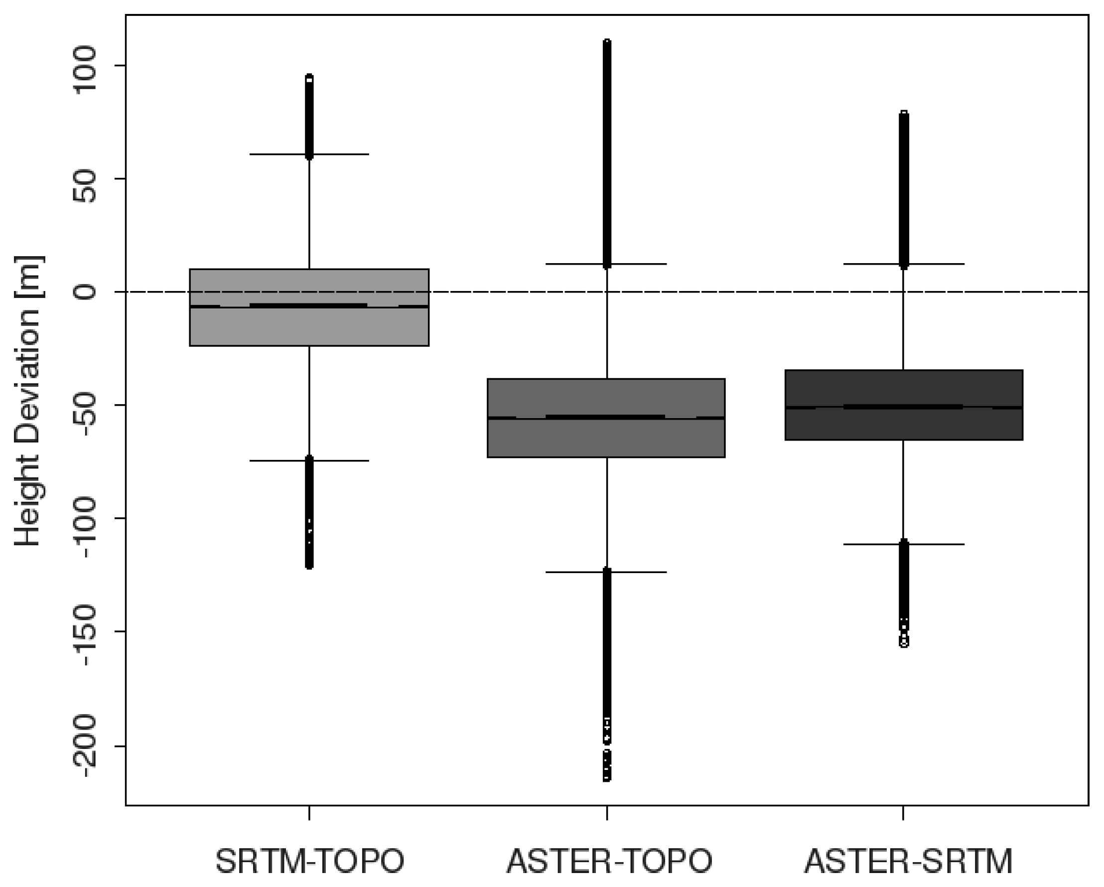
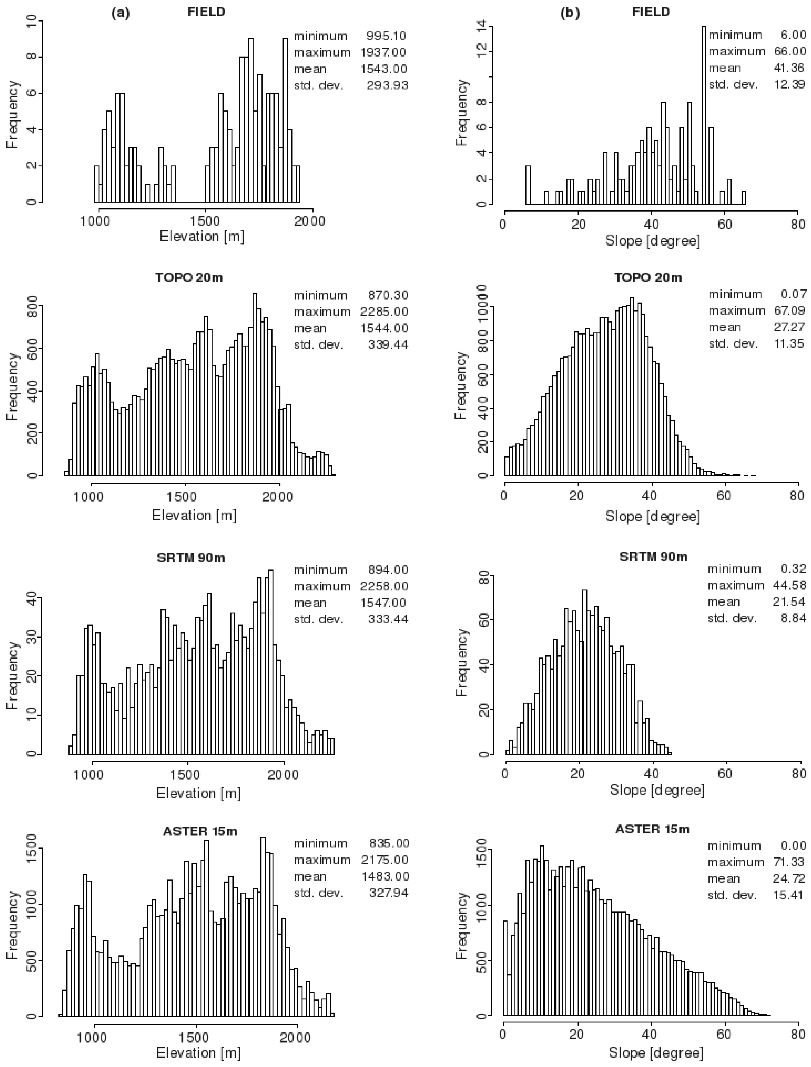
3.1. Elevation

| RMSE | TOPO DEM | SRTM DEM | ASTER DEM | ||
|---|---|---|---|---|---|
| Resolution | 20-m | 20-m | 90-m | 20-m | 15-m |
| Elevation [m] | 53.47 | 50.60 | 52.72 | 69.76 | 70.94 |
| Slope [°] | 19.60 | 18.15 | 21.39 | 20.89 | 21.31 |
| LS factor | 47.75 | 47.65 | 41.67 | 35.88 | 33.10 |
| Minimum | Maximum | Mean | Standard deviation | |
|---|---|---|---|---|
| TOPO 20m | −155.00 | 105.20 | 4.40 | 53.46 |
| SRTM 20m | −155.50 | 76.70 | −13.21 | 49.00 |
| SRTM 90m | −164.30 | 96.33 | −12.56 | 51.37 |
| ASTER 20m | −161.70 | 10.15 | −57.20 | 39.83 |
| ASTER 15m | −156.80 | 7.41 | −58.66 | 40.02 |
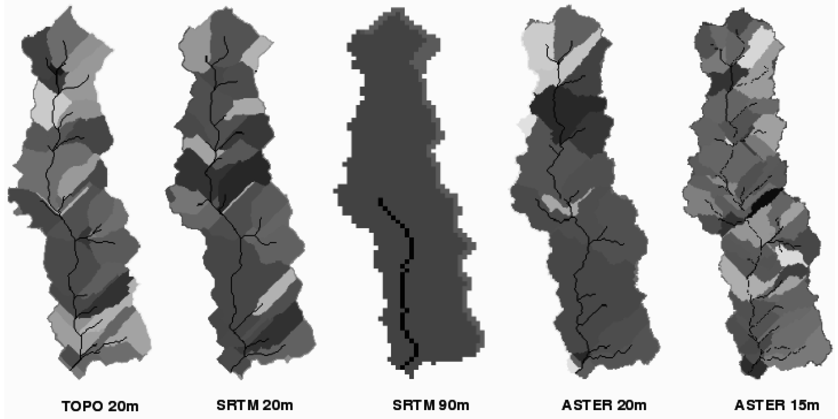
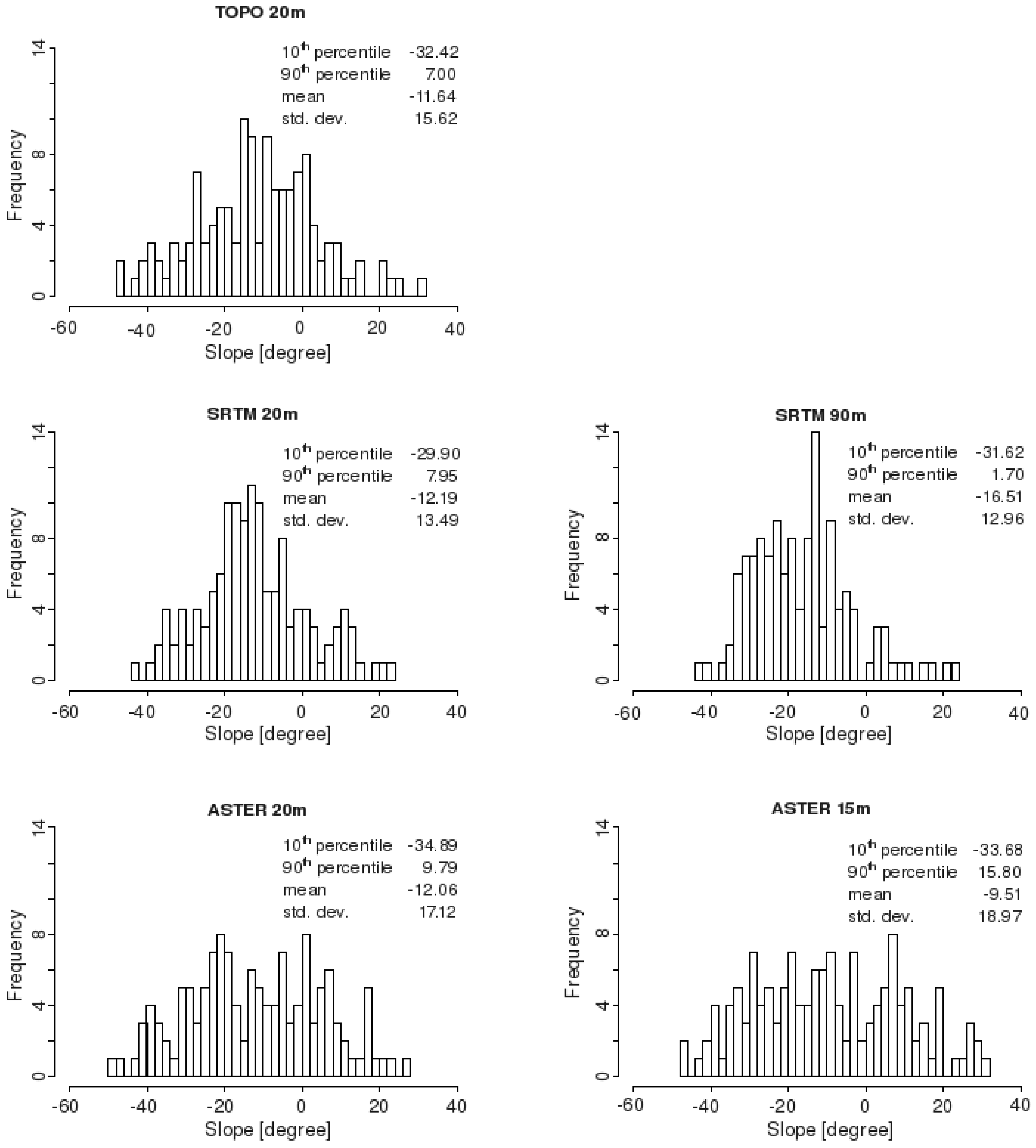
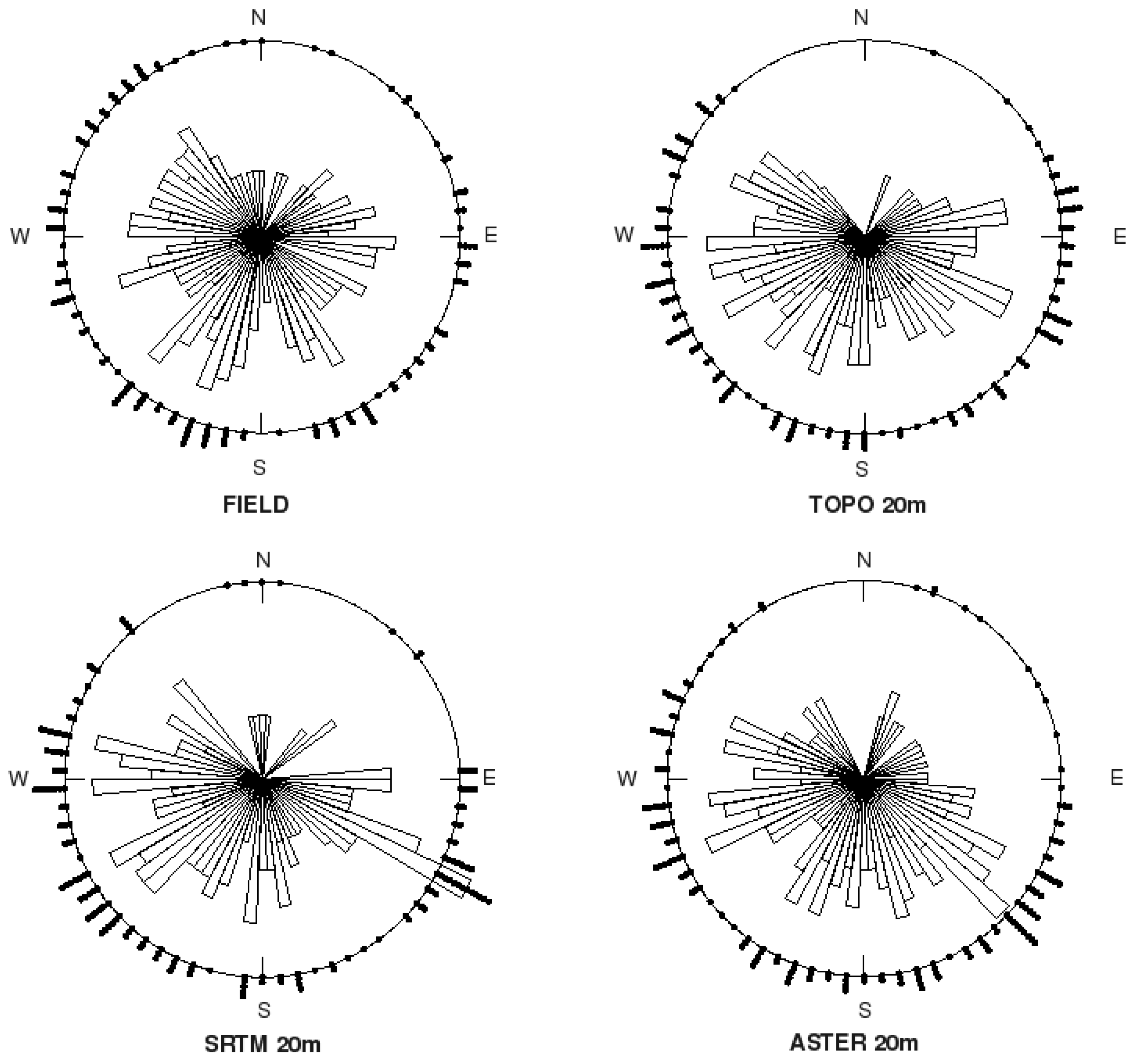
3.2. Slope, Aspect and Channels


| DEM | Area (ha) | No. of hillslopes | No. of channels |
|---|---|---|---|
| TOPO 20m | 1249.6 | 21 | 37 |
| SRTM 20m | 1276.4 | 21 | 26 |
| SRTM 90m | 1275.1 | 3 | 1 |
| ASTER 20m | 1226.3 | 23 | 29 |
| ASTER 15m | 1227.7 | 28 | 53 |
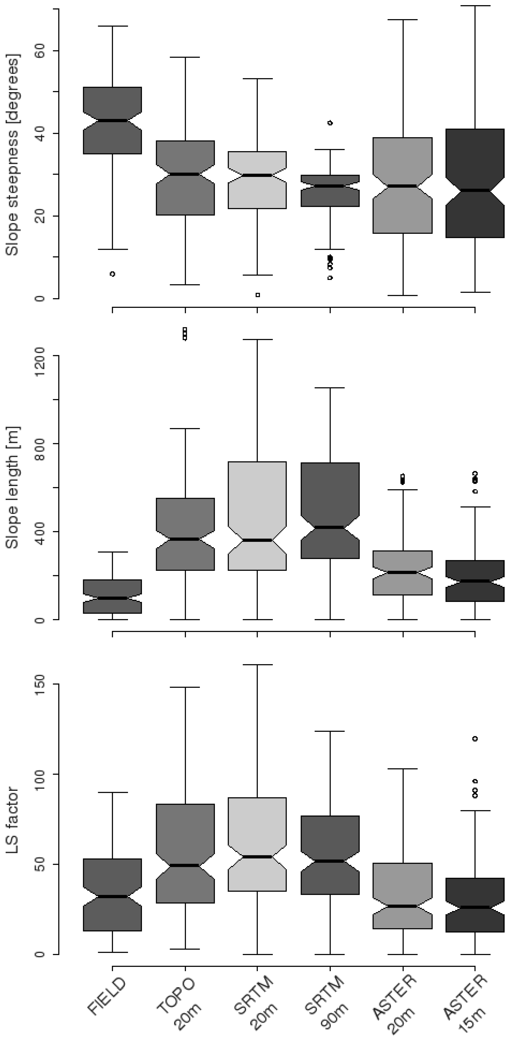
3.3. RUSLE LS Factors

| Minimum | Maximum | Mean | Median | Standard deviation | |
|---|---|---|---|---|---|
| FIELD | 0.95 | 89.56 | 34.62 | 31.92 | 23.52 |
| TOPO 20m | 2.75 | 148.20 | 57.26 | 48.71 | 36.42 |
| SRTM 20m | 0 | 160.80 | 61.32 | 53.80 | 36.22 |
| SRTM 90m | 0 | 123.40 | 54.09 | 51.52 | 29.27 |
| ASTER 20m | 0 | 102.70 | 34.39 | 26.54 | 25.28 |
| ASTER 15m | 0 | 119.60 | 30.27 | 25.60 | 23.18 |
4. Discussion
4.1. DEM Elevation
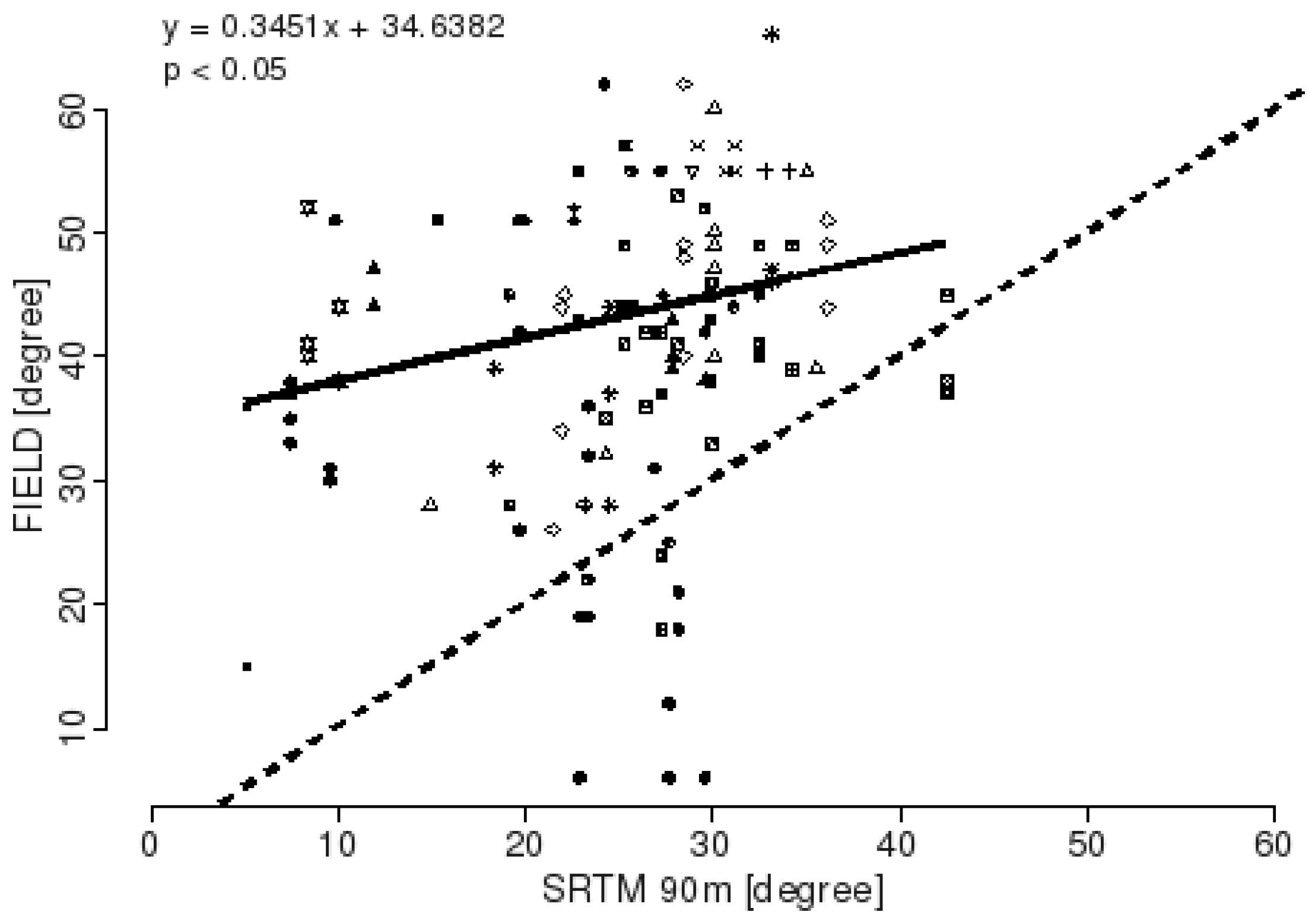
4.2. Slope and Aspect
4.3. RUSLE LS Factor
5. Conclusions
Acknowledgements
References
- Lal, R. Soil degradation by erosion. Land Degrad. Dev. 2001, 12, 519–539. [Google Scholar] [CrossRef]
- Zhang, J.X.; Chang, K.-T.; Wu, J.Q. Effects of DEM resolution and source on soil erosion modelling: A case study using the WEPP model. Int. J. Geogr. Inf. Sci. 2008, 22, 925–942. [Google Scholar] [CrossRef]
- Sefercik, U.; Jacobsen, K.; Oruc, M.; Marangoz, A. Comparison of SPOT, SRTM and ASTER DEMs. In Proceedings of the ISPRS Workshop on High-Resolution Earth Imaging for Geospatial Information, Hannover, Germany, 29 May–1 June 2007.
- Rabus, B.; Eineder, M.; Roth, A.; Bamler, R. The shuttle radar topography mission—A new class of digital elevation models acquired by spaceborne radar. ISPRS J. Photogramm. Remote Sens. 2003, 57, 241–262. [Google Scholar] [CrossRef]
- Abrams, M. ASTER: Data products for the high spatial resolution imager on NASA’s Terra platform. Int. J. Remote Sens. 2000, 21, 847–853. [Google Scholar] [CrossRef]
- Eckholm, E. The deterioration of mountain environments. Science 1975, 189, 764–770. [Google Scholar] [CrossRef] [PubMed]
- Reiger, H.C. Man versus mountain: The destruction of the Himalayan ecosystem. In The Himalaya: Aspects of Change; Lal, J.S., Moddie, A.D., Eds.; Oxford University Press: New Delhi, India, 1981; pp. 351–376. [Google Scholar]
- Myers, N. Environmental repercussions of deforestation in the Himalayas. J. World Forest Resource Manag. 1986, 2, 63–72. [Google Scholar]
- Shrestha, D.P. Assessment of soil erosion in the Nepalese Himalaya, a case study in Likhu Khola valley, Middle Mountain region. In Land Husbandry; Oxford & IBH Publishing Co. Pvt. Ltd.: New Delhi, India, 1997; Volume 2, pp. 59–80. [Google Scholar]
- Morgan, R.P.C.; Morgan, D.D.V.; Finney, H.J. A predictive model for the assessment of soil erosion risk. J. Agr. Eng. Res. 1984, 30, 245–253. [Google Scholar] [CrossRef]
- Kumar, S.; Sharma, S. Soil erosion risk assessment based on MMF model using remote sensing and GIS. Hydrology J. 2005, 28, 47–58. [Google Scholar]
- Jain, S.K.; Kumar, S.; Varghese, J. Estimation of soil erosion for a Himalayan watershed using GIS technique. Water Resour. Manag. 2001, 15, 41–54. [Google Scholar] [CrossRef]
- Wischmeier, W.H.; Smith, D.D. Predicting Rainfall Erosion Losses—A Guide to Conservation Planning; Agricultural Handbook No. 537; U.S. Department of Agriculture, Agricultural Research Service: Washington, DC, USA, 1978.
- Hessel, R.; Gupta, M.K.; Datta, P.S.; Gelderman, E. Application of the LISEM soil erosion model to a forested catchment in the Indian Himalayas. Int. J. Ecol. Environ. Sci. 2007, 33, 129–142. [Google Scholar]
- De Roo, A.P.J.; Wesseling, C.G.; Ritsema, C.J. LISEM: A single-event physically based hydrological and soil erosion model for drainage basins. I: Theory, input and output. Hydrol. Process. 1996, 10, 1107–1117. [Google Scholar] [CrossRef]
- Jetten, V.; De Roo, A.P.J. Spatial analysis of erosion conservation measures with LISEM. In Landscape Erosion and Evolution Modeling; Harmon, R., Doe, W.W., Eds.; Kluwer Academic/Plenum: New York, NY, USA, 2001; pp. 429–445. [Google Scholar]
- de Vente, J.; Poesen, J.; Govers, G.; Boix-Fayos, C. The implications of data selection for regional erosion and sediment yield modelling. Earth Surf. Process. Landf. 2009, 34, 1994–2007. [Google Scholar] [CrossRef]
- Jenson, S.K. Applications of hydrological information automatically extracted from digital elevation models. Hydrol. Process. 1991, 5, 31–44. [Google Scholar] [CrossRef]
- Wolock, D.M.; McCabe, G. Differences in topographic characteristics computed from 100- and 1000-m resolution digital elevation model data. Hydrol. Process. 2000, 14, 987–1002. [Google Scholar] [CrossRef]
- Raina, A.K.; Gupta, M.K. Geology and geomorphology of Arnigad watershed in Lesser Himalayas, Missoorie Forest Division, Uttaranchal. Ann. Forest. 2006, 14, 255–267. [Google Scholar]
- Sharma, S.D.; Singh, B.R.; Sitaula, B.; Gupta, M.K. Influence of land cover on soil properties in a watershed in Lesser Himalayas. Ann. Forest. 2006, 14, 16–34. [Google Scholar]
- Chandra, R.; Soni, P.; Yadav, V. Fuelwood, fodder and livestock status in a Himalayan watershed in Mussoorie Hills (Uttarakhand), India. Indian Forest. 2008, 134, 894–905. [Google Scholar]
- Hirano, A.; Welch, R.; Lang, H. Mapping from ASTER stereo image data: DEM validation and accuracy assessment. ISPRS J. Photogramm. Remote Sens. 2003, 57, 356–370. [Google Scholar] [CrossRef]
- USGS. Shuttle Radar Topography Mission, 3 Arc Second Scene SRTM_ff03_p146r039, Filled Finished-A; Global Land Cover Facility, University of Maryland: College Park, MD, USA, February 2000.
- Mitasova, H.; Hofierka, J. Interpolation by regularized spline with tension: II. Application to terrain modeling and surface geometry analysis. Math. Geol. 1993, 25, 657–669. [Google Scholar] [CrossRef]
- Mitasova, H.; Mitas, L. Interpolation by regularised spline with tension: I. Theory and implementation. Math. Geol. 1993, 25, 641–655. [Google Scholar] [CrossRef]
- Jenson, S.K.; Domingue, J.O. Extracting topographic structure from digital elevation data for geographic information system analysis. Photogramm. Eng. Remote Sensing 1988, 54, 1593–1600. [Google Scholar]
- Neteler, M.; Mitasova, H. Open Source GIS—A GRASS GIS Approach, 3rd ed.; Springer: New York, NY, USA, 2007; Volume 773. [Google Scholar]
- Nikolakopoulos, K.G.; Kamaratakis, E.K.; Chrysoulakis, N. SRTM vs ASTER elevation products. Comparison for two regions in Crete, Greece. Int. J. Remote Sens. 2006, 27, 4819–4838. [Google Scholar] [CrossRef]
- Horn, B. Hill shading and the reflectance map. Proc. IEEE 1981, 69, 14–47. [Google Scholar] [CrossRef]
- Renard, K.G.; Foster, G.R.; Weesies, G.A.; McCool, D.K.; Yoder, D.C. Predicting Soil Erosion by Water: A Guide to Conservation Planning with the Revised Universal Soil Loss Equation (RUSLE); Agriculture Handbook No. 703; US Department of Agriculture, Agricultural Research Service: Washington, DC, USA, 1997.
- Renard, K.G.; Ferreira, V.A. RUSLE model description and database sensitivity. J. Environ. Qual. 1993, 22, 458–466. [Google Scholar] [CrossRef]
- McCool, D.K.; Foster, G.R.; Mutchler, C.K.; Meyer, L.D. Revised slope length factor for the Universal Soil Loss Equation. Trans. ASAE 1989, 32, 1571–1576. [Google Scholar] [CrossRef]
- McCool, D.K.; Brown, C.L.; Foster, G.R.; Mutchler, C.K.; Meyer, L.D. Revised slope steepness factor for the Universal Soil Loss Equation. Trans. ASAE 1987, 30, 1387–1396. [Google Scholar] [CrossRef]
- Eckert, S.; Kellenberger, T. Qualitätanalyse automatisch generierter digitaler Geländenodelle aus ASTER Daten. In Proceedings of Wissenschaftlich-Technische Jahrestagung der Deutschen Gesellschaft für Photogrammetrie und Fernerkundung, Neubrandenburg, Germany; 2002; pp. 337–341. [Google Scholar]
- Eckert, S.; Kellenberger, T.; Itten, K. Accuracy assessment of automatically derived digital elevation models from aster data in mountainous terrain. Int. J. Remote Sens. 2005, 26, 1943–1957. [Google Scholar] [CrossRef]
- Kamp, U.; Bolch, T.; Olsenholler, J. Geomorphometry of Cerro Sillajhuay (Andes, Chile/Bolivia): Comparison of digital elevation models (DEMs) from ASTER remote sensing data and contour maps. Geocarto Int. 2005, 20, 23–33. [Google Scholar] [CrossRef]
- Toutin, Th. 3D topographic mapping with ASTER stereo data in rugged topography. IEEE Trans. Geosci. Remote Sens. 2002, 40, 2241–2247. [Google Scholar] [CrossRef]
- Gallant, J.C.; Wilson, J.P. Primary topographic attributes. In Terrain Analysis: Principles and Applications; Wilson, J.P., Gallant, J.C., Eds.; John Wiley and Sons: New York, NY, USA, 2000; pp. 51–85. [Google Scholar]
- Huggel, C.; Schneider, D.; Miranda, P.J.; Granados, H.D.; Kääb, A. Evaluation of ASTER and SRTM DEM data for lahar modelling: A case study on lahars from Popocatépetl volcano, Mexico. J. Volcan. Geotherm. Res. 2008, 170, 99–110. [Google Scholar] [CrossRef] [Green Version]
- Gorokhovich, Y.; Voustianiouk, A. Accuracy assessment of the processed SRTM-based elevation data by CGIAR using field data from USA and Thailand and its relation to the terrain characteristics. Remote Sens. Environ. 2006, 104, 409–415. [Google Scholar] [CrossRef]
- Kääb, A. Combination of SRTM3 and repeat ASTER data for deriving alpine glacier flow velocities in the Bhutan Himalaya. Remote Sens. Environ. 2005, 94, 463–474. [Google Scholar] [CrossRef]
- Wolock, D.M.; Price, C.V. Effects of digital elevation map scale and data resolution on a topographically-based watershed model. Water Resour. Res. 1994, 30, 3041–3052. [Google Scholar] [CrossRef]
- Zhang, W.H.; Montgomery, D.R. Digital elevation model grid size, landscape representation, and hydrologic simulations. Water Resour. Res. 1994, 30, 1019–1028. [Google Scholar] [CrossRef]
- Kienzle, S. The effect of DEM raster resolution on first order, second order and compound terrain derivatives. Trans. GIS 2004, 8, 83–111. [Google Scholar] [CrossRef]
- Bolstad, P.V.; Stowe, T. An evaluation of DEM Accuracy: Elevation, slope, and aspect. Photogramm. Eng. Remote Sensing 1994, 60, 1327–1332. [Google Scholar]
- SAS Institute Inc. SAS/STAT Software Version 9.1; SAS Institute Inc.: Cary, NC, USA, 2008. [Google Scholar]
- van Remortel, R.D.; Hamilton, M.E.; Hickey, R.J. Estimating the LS factor for RUSLE through iterative slope length processing of digital elevation data within ArcInfo grid. Cartography 2001, 30, 27–35. [Google Scholar] [CrossRef]
© 2010 by the authors; licensee MDPI, Basel, Switzerland. This article is an Open Access article distributed under the terms and conditions of the Creative Commons Attribution license (http://creativecommons.org/licenses/by/3.0/).
Share and Cite
Datta, P.S.; Schack-Kirchner, H. Erosion Relevant Topographical Parameters Derived from Different DEMs—A Comparative Study from the Indian Lesser Himalayas. Remote Sens. 2010, 2, 1941-1961. https://doi.org/10.3390/rs2081941
Datta PS, Schack-Kirchner H. Erosion Relevant Topographical Parameters Derived from Different DEMs—A Comparative Study from the Indian Lesser Himalayas. Remote Sensing. 2010; 2(8):1941-1961. https://doi.org/10.3390/rs2081941
Chicago/Turabian StyleDatta, Pawanjeet S., and Helmer Schack-Kirchner. 2010. "Erosion Relevant Topographical Parameters Derived from Different DEMs—A Comparative Study from the Indian Lesser Himalayas" Remote Sensing 2, no. 8: 1941-1961. https://doi.org/10.3390/rs2081941