Article

Investigation on the Patterns of Global Vegetation Change Using a Satellite-Sensed Vegetation Index

1
Institute of Mountain Hazards and Environment, Chinese Academy of Sciences, Chengdu, Sichuan 610041, China
2
Department of Geography, University of Maryland, College Park, MD 20742, USA
*
Author to whom correspondence should be addressed.
Remote Sens. 2010, 2(6), 1530-1548; https://doi.org/10.3390/rs2061530
Submission received: 2 April 2010 / Revised: 18 May 2010 / Accepted: 21 May 2010 / Published: 3 June 2010
(This article belongs to the Special Issue Ecological Status and Change by Remote Sensing)

Abstract

:
The pattern of vegetation change in response to global change still remains a controversial issue. A Normalized Difference Vegetation Index (NDVI) dataset compiled by the Global Inventory Modeling and Mapping Studies (GIMMS) was used for analysis. For the period 1982–2006, GIMMS-NDVI analysis indicated that monthly NDVI changes show homogenous trends in middle and high latitude areas in the northern hemisphere and within, or near, the Tropic of Cancer and Capricorn; with obvious spatio-temporal heterogeneity on a global scale over the past two decades. The former areas featured increasing vegetation activity during growth seasons, and the latter areas experienced an even greater amplitude in places where precipitation is adequate. The discussion suggests that one should be cautious of using the NDVI time-series to analyze local vegetation dynamics because of its coarse resolution and uncertainties.

1. Introduction

Vegetation is the dominant component of terrestrial ecosystems, which play a vital role in the cycle of global resources and energy [1]. Furthermore, it has an irreplaceable function in regulating global carbon balance and maintaining global climate stability [2,3]. As a global change issue, the vegetation growth response to climate change has gained much more attention [4], since it has become an urgent necessity for countries to estimate carbon uptake on a continental scale.
In recent years, various approaches have proved the existence of a terrestrial carbon sink, with a geographical distribution and magnitude that is still under discussion [5,6]. Studies of the ecosystem response to gas exchange at the site level [7], forest inventories at the continental level [8], and tracer transport inversion methods at the global level [9,10] have all suggested a net gain of carbon in terrestrial ecosystems. Meanwhile, some research studies (e.g., [11]) have revealed that the response of vegetation to global change has obvious geographical heterogeneity and different phases. For instance, vegetation activities at mid-high latitude in the northern hemisphere increased dramatically during the past decades [12,13]. This phenomenon is attributed to two factors: (1) carbon dioxide accumulation in the atmosphere causing a rise in temperature; and (2) sequestration of soil nitrogen and phosphorus leading to vegetation vigor varied with greater periodic oscillation [14]. On the other hand, global warming resulted in earlier and prolonged vegetation growth seasons [15]. However, a few time-series data for a 100 year period indicated that the spring phenophase was prone to delay during certain periods of time [16]. That is to say, the response of vegetation in some regions to global change is mainly reflected by longer growing periods, while in other regions, ecosystems respond with greater amplitude in vegetation vigor, or include both features mentioned above. Obviously, on a global spatial scale and decadal temporal scale, differing theories on the vegetation response to global change still exist. While the earth’s surface has undergone unprecedented warming over the last two decades, since reliable instrumental measurements became available in the late 19th Century [17], there are still some reports on regional cooling. Therefore, investigating the spatial-temporal pattern of vegetation change over the world in recent decades is necessary for obtaining a greater understanding of global change and the corresponding vegetation response.
Among satellite remote sensing data, the NOAA-AVHRR sensor provides the longest time-series of satellite images for global vegetation dynamics analysis. The Normalized Difference Vegetation Index (NDVI), a spectral index linearly related to the fraction of the photosynthetically active radiation (400–700 nm) intercepted by the canopy [18,19], has proven to be a proxy for the status of the aboveground biomass at the landscape level. This is due to the high correlation with green-leaf density, photosynthesis intensity, net primary production and carbon dioxide fluxes [20,21]. Therefore, it is usually applied directly for study of vegetation dynamics. More frequently, the well-known maximum value composites of daily NDVI data [22] are used to reduce the influence of atmospheric effects on images. Many researchers (e.g., [23,24,25,26]) have successfully utilized the AVHRR time-series NDVI to study vegetation growth in terms of time and space.
Typically an NDVI time-series is characterized by patterns like seasonality, trends and localized abrupt changes, or discontinuities, resulting from disturbance events [27]. The remote sensing techniques based on time-series analysis facilitates the characterization of inter-annual and intra-annual variations of the vegetation canopy [28]. The inter-annual changes in vegetation dynamics also contain valuable information on the response of vegetation to meteorological effects. However, as aforementioned, vegetation change on the global scale features high geographical heterogeneity and is non-stationary. Here we focus on those stationary changes and trends between years over the long time-series, excluding non-stationary processes, since the continuous and stable changes are likely the response to the micro global climate change [29].
The methods for analyzing the NDVI time-series include statistical approaches such as principal component analysis [30,31] and curve fitting [32], as well as spectral-frequency techniques such as Fourier analysis [33], harmonic analysis [34] and wavelet decomposition [35,36]. In this paper, we use the time-series AVHRR-NDVI archives (1982–2006) to investigate global monthly vegetation stability change trends, by means of empirical orthogonal function (EOF) analysis. The analysis seeks to prove large-scale variation and spatial-temporal heterogeneity of global vegetation vigor, and to answer the following questions: (1) where and when did the vegetation vigor change with a stable trend during the last two decades; (2) how did the vegetation change in response to global climate change? For such a purpose, the time-series NDVI was first smoothed by a Savitzky-Golay (S-G) filter to remove deviations from the vegetation cycle. The monthly NDVI anomalies were then calculated and stacked as a monthly time-series anomaly layers. Finally, an EOF analysis was conducted against the monthly NDVI anomalies to extract the overall change trend across the world in the last two decades. The likely vegetation response to the global climate change and limitations of our study are also discussed further.

2. Materials and Methods

2.1. Data and Processing
The analyses were based on NDVI data derived from the Advance Very High Resolution Radiometer (AVHRR) sensor on board the National Oceanic and Atmospheric Agency (NOAA) satellite. The NDVI was calculated as the difference between the reflectance registered by the AVHRR sensor in the near-infrared and visible portion of the electromagnetic spectrum divided by the sum of both channels. A NDVI dataset compiled by the Global Inventory Modeling and Mapping Studies (GIMMS) was adopted. The GIMMS-NDVI data were generated to provide a more than 25-year (July, 1981–December, 2006) satellite record of monthly changes in terrestrial vegetation, with a spatial resolution of 8 km × 8 km and a temporal resolution of 15-Days. The dataset can be obtained from the Global Land Cover Facility (GLCF) (ftp://ftp.glcf.umiacs.umd.edu). The geographic coordinates version supplied by GLCF as one global mosaic is convenient for researchers to model the globe during a single analysis. The GIMMS-NDVI dataset has been used in various models and appears to capture general patterns of vegetation well [37,38]. Tests on sites indicate reasonable agreement between the inter-annual variation in GIMMS NDVI and other measures of vegetation [38,39,40,41,42]. These tests show that the variation in GIMMS NDVI is realistic on specific sites.
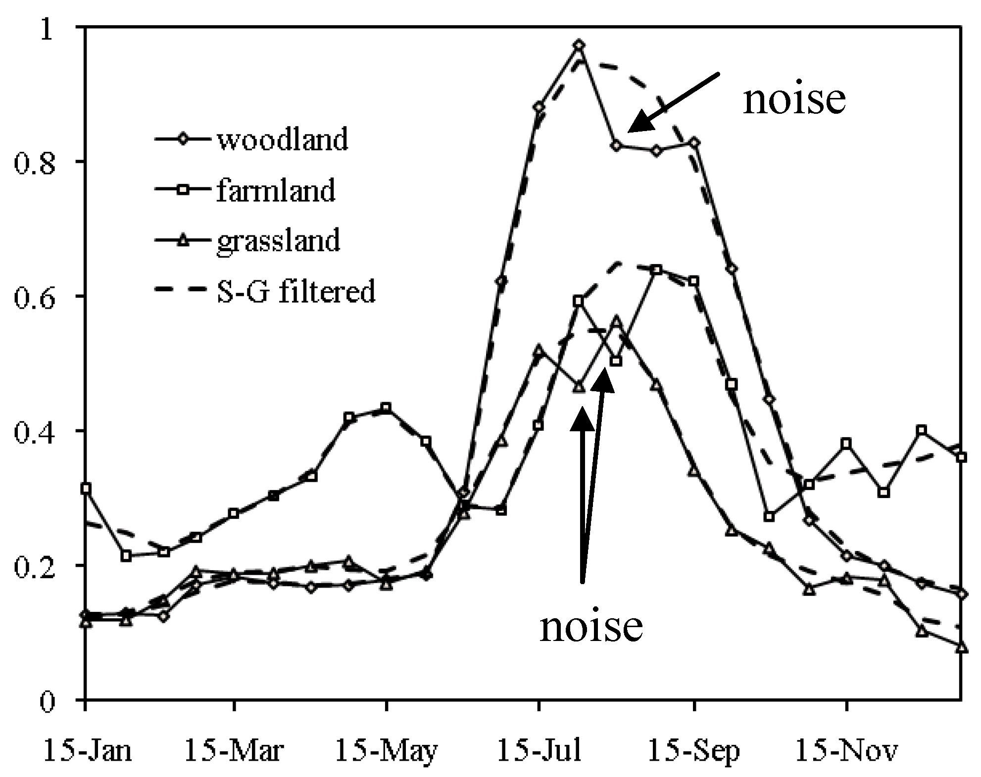
However, in the NDVI time-series, there are always disturbances created by cloud contamination, atmospheric variability, bi-directional effects and sensor malfunctions [43,44]. Although Maximum Value Composite (MVC) products can partly eliminate some disturbances [22,45], the time-series NDVI data still includes many of these deviations (see Figure 1). Thus, prior to the analysis of the time series NDVI, the dataset must be pre-processed to remove such disturbances. In this study, the Savitzky-Golay (S-G) filter is applied to smoothen the noise in the NDVI time-series. The S-G filter is a simplified least-squares-fit convolution for smoothing and computing derivatives of a set of consecutive values (a spectrum) [46], and has been successfully used to reconstruct the NDVI time-series data in several recent researches [47,48]. The general equation of the simplified least-squares convolution for an NDVI time series smoothing is given as:
Y j = i = m i = m C i Y j + i N
where Yj+i is the original NDVI value, Yj is the resultant NDVI value, Ci is the coefficient for the ith NDVI value of the filter (smoothing window). It can be obtained directly from Steinier et al. [49] as a corrected version of Savitzky and Golay’s work [46]. N is the number of convoluting integers and is equal to the smoothing window size (2m + 1). The smoothing array (filter size) consists of 2m+ 1 points, where m is the half-width of the smoothing window, and is set as 4 for our study. The typical filtered NDVI profiles obtained are shown in Figure 1.
When the NDVI value is comparatively small (close to 0), using it to detect a change can lead to relatively large errors [50]. In this study we chose the NDVI pixel values that are greater than 0.1 to represent vegetation vigor, and chose the value at the end of each month to represent the monthly NDVI data. Because the GIMMS-NDVI can only be acquired partially for 1981 (July–December), the dataset was arranged as monthly NDVI across the globe on a 8 km × 8 km regular grid and spans the period 1982–2006. The mean annual cycle was calculated by averaging the monthly data over the years, and any anomalies were then computed as a departure from the mean annual cycle in order to remove long-term variations in multi-temporal NDVI change. An anomaly is considered a deviation from an inner trend, which is the indicator for evaluating NDVI inter-annual change.
Figure 1. The GIMMS-NDVI temporal profiles for several typical vegetation classes in the north mid-high latitude area. Noise points, original profiles, and smoothed profiles from the S-G filter are shown as examples.
Remotesensing 02 01530 g001

2.2. Extracting the Spatial-Temporal Change by Using an Empirical Orthogonal Function (EOF) Method

This paper focuses primarily on revealing the spatio-temporal patterns of the NDVI stable change trend during 1982–2006, which is likely caused by the global durative micro-climate change in the last several decades. In a growth season, the change trend between months is also investigated, which can reflect the regional growth season change. Although the monthly NDVI anomaly can indicate deviation from the long term cycle, we cannot reliably identify the continuous change trend from a single anomaly image. This paper uses an empirical orthogonal function (EOF) analysis to extract monthly NDVI change tendencies from the monthly time-series NDVI anomalies, because EOF offers a clear advantage in analyzing spatial-temporal changes [51]. EOF analysis uses properties of matrix algebra to decompose a dataset into spatially orthogonal Eigen-functions and associated temporal coefficients, and is among the most widely used methods in meteorological science [52,53]. With the space-time field, EOF analysis finds a set of orthogonal spatial patterns, known as EOFs, along with a set of associated uncorrelated time-series or PCs, so that the first few PCs account for as much as possible the variation in the original field [54]. This allows for the extraction of the main change trend, which explains the maximum amount of variance in the dataset, by combining the first several PCs. Therefore, EOF has been used most recently in the NDVI time-series analysis [55,56,57,58].
Mathematically, the purpose of an EOF analysis is to replace p observed variables by a much smaller number k of uncorrelated principal components, while retaining as the most possible variation in the original p variables.
For example, let X R n × p denote a gridded dataset containing n time samples for monthly NDVI anomalies measured by their means at p grid-points. The EOFs can easily be computed by using the singular value decomposition (SVD) [59]. Assume that X has rank r with r ≤ min (n,p). Using the SVD, X can be decomposed as:
X = M Λ U = j = 1 r λ j m j u j
where M = ( m 1 , ... , m r ) R n × r and U = ( u 1 , ... , u r ) R p × r are orthonormal matrices; so that M M = U U = I r , with I r as an identity matrix of order r; and Λ R r × r is a diagonal matrix with the singular values of X, sorted in decreasing order, λ 1 λ 2 ... λ r 0 , on its main diagonal. The prime notation stands for the transpose operator. The matrix U in Equation (2) is the matrix of the EOFs, and M Λ is the matrix of PC scores. The variance of the j th PC, j = 1 , ... , r , is λ j 2 / ( n 1 ) , which is equal to the j th eigenvalue of the sample covariance matrix of X. In practice, the first leading k components, with k r , account for a substantial proportion of the total variance in the data (e.g., 60%), and the sum in the equation is therefore truncated after the first k terms. Thus, an EOF analysis is dependent upon finding a n × k real matrix of component scores of the n time samples on the k components, and a loading matrix U R p × k containing the EOF coefficients for the p grid points on the k components.
Figure 2. Overall data flow and processes of EOF analysis.
Remotesensing 02 01530 g002
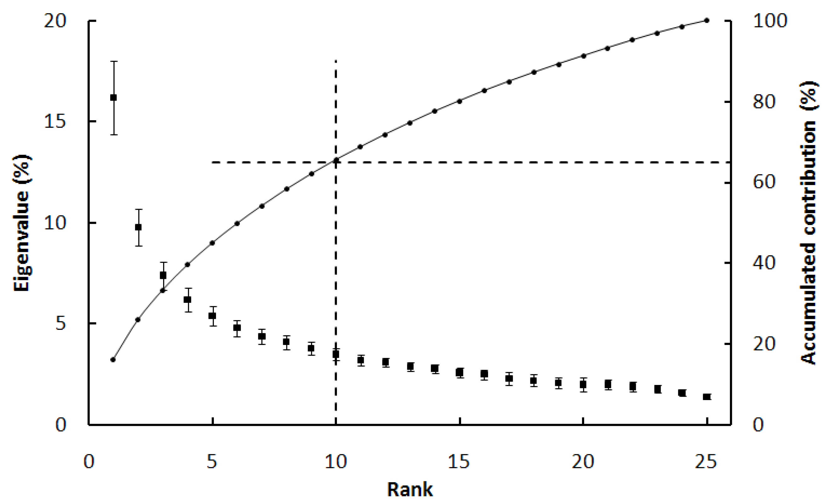
In this study, n is the 25 year period of 1982 to 2006, and p is the monthly global NDVI anomaly images, containing 4,950 columns × 2,091 rows pixels. EOF analysis is applied to decompose 25 NDVI image anomalies for each month. For instance, the NDVI anomalies of January from 1982 to 2006 were used to operate the EOF analysis to extract the homogeneous change trend in January for this period. This NDVI change pattern study is based on the composition of k components. The overall method consists of five major steps (Figure 2): GIMMS NDVI S-G filtering processing, calculating monthly NDVI anomalies, EOF analysis based on each monthly stack, leading principal components compositing, and global NDVI change pattern analysis. Figure 3 shows the result of the monthly NDVI anomaly image spectrum, expressed in percent of explained variance of the EOFs, along with the standard error computed from 12 monthly EOF analyses (from January to December). The first ten EOFs (k = 10), can explain around 65% of the total variance in the global monthly NDVI during the last two decades (see Figure 3); therefore, the first 10 PCs were composited to reflect the dominating monthly NDVI change on a global scale. On this basis, we can extract regions within a time series where similar NDVI dynamic change and spatial patterns appear.
Figure 3. Spectrum of the covariance matrix of monthly global NDVI anomalies, and the accumulated percentage of Eigenvalue. Vertical bars show the standard deviation of the percentage Eigenvalue over 12 months (January-December) by EOF analysis. The Eigenvalue percentage is the ratio of an individual Eigen-value to the sum of all Eigenvalues.
Remotesensing 02 01530 g003

2.3. The Hypotheses of Vegetation Change Analysis

In order to investigate the dominating response of vegetation activities in different regions to global change, as well as its spatial patterns, our analysis is based on the following hypotheses: (1) In regions with the highest NDVI rate increase in spring, the vegetation response to global change is primarily shown through the early start of the growing season. (2) In regions with the highest NDVI rate increase in the summer, the response is primarily shown through greater amplitude or enhanced vegetation vigor in the growth season. (3) In regions with the highest NDVI rate increase in autumn, the response shows an obvious extension of vegetation growth season. Most of these hypotheses are verified in recent related research studies [13]. Furthermore, in the temperate zone the season can be divided into spring, summer, autumn and winter (see Table 1). Normally, the growth season is from spring to autumn, and the specific dates vary with the latitude. Summer is the flourishing season and winter is non-flourishing season for vegetation growth. Vegetation grows abundantly throughout the entire year within the tropical zone, with growth season changes mainly present out of the tropical area. Therefore, the analysis of vegetation changes in the tropical zone focus on the amplitude of the vigor variation.
Table 1. The division of season for North Hemisphere and South Hemisphere according to temperate zone.
MonthJanFebMarAprMayJunJulAugSepOctNovDec
North hemisphereWinterSpringSummerAutumnWinter
South hemisphereSummerAutumnWinterSpringSummer

3. Results and Analysis

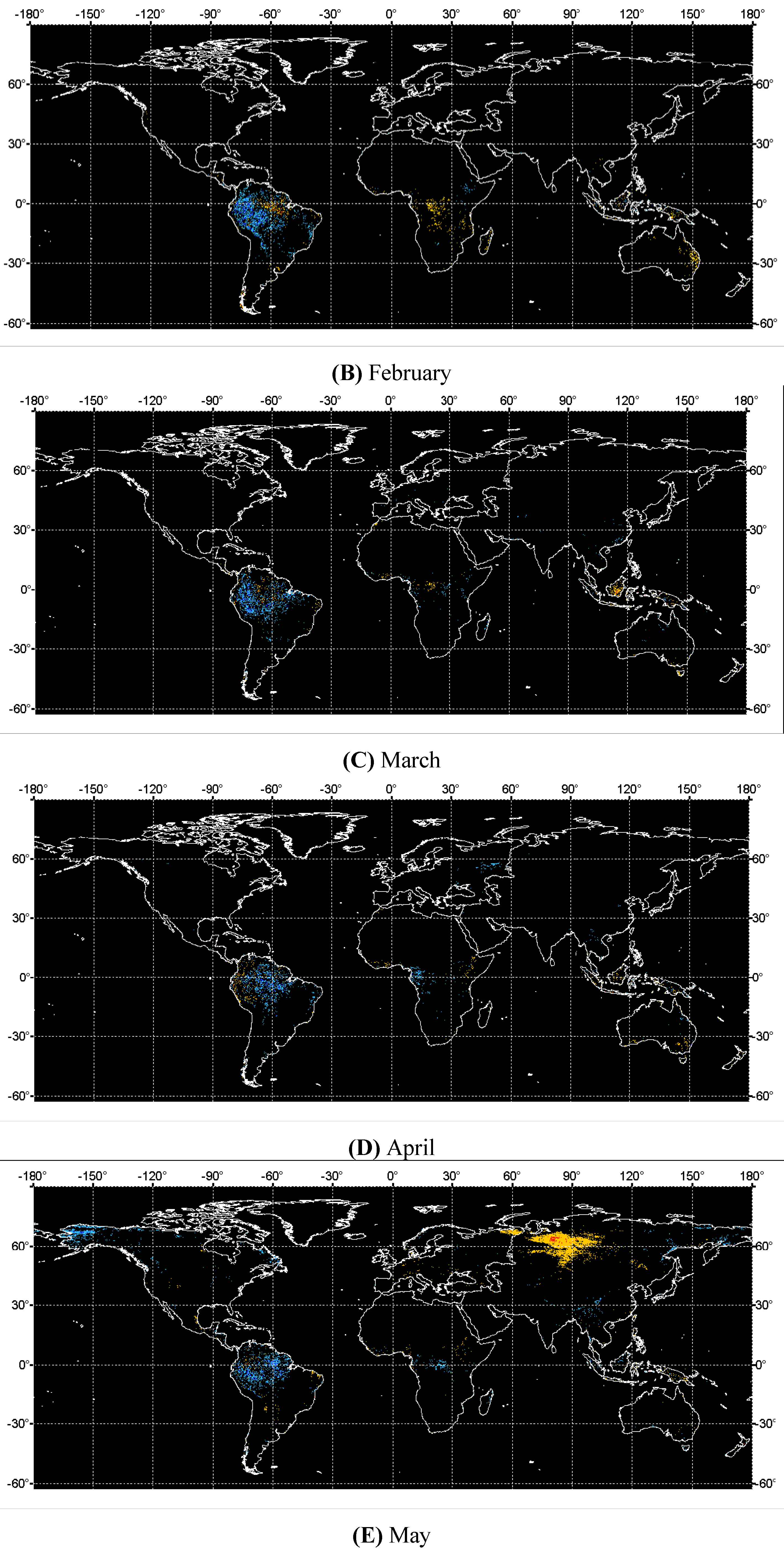
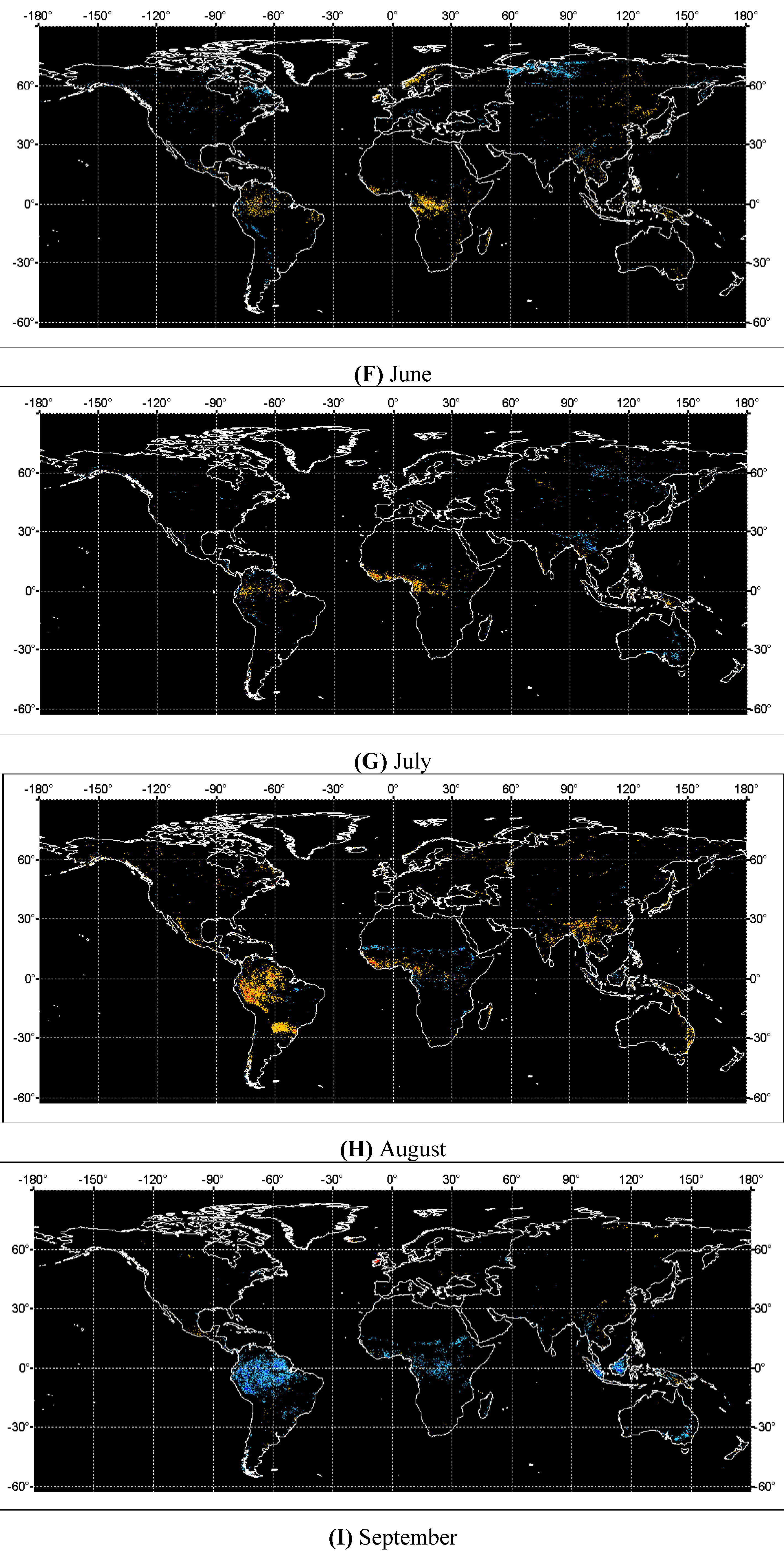
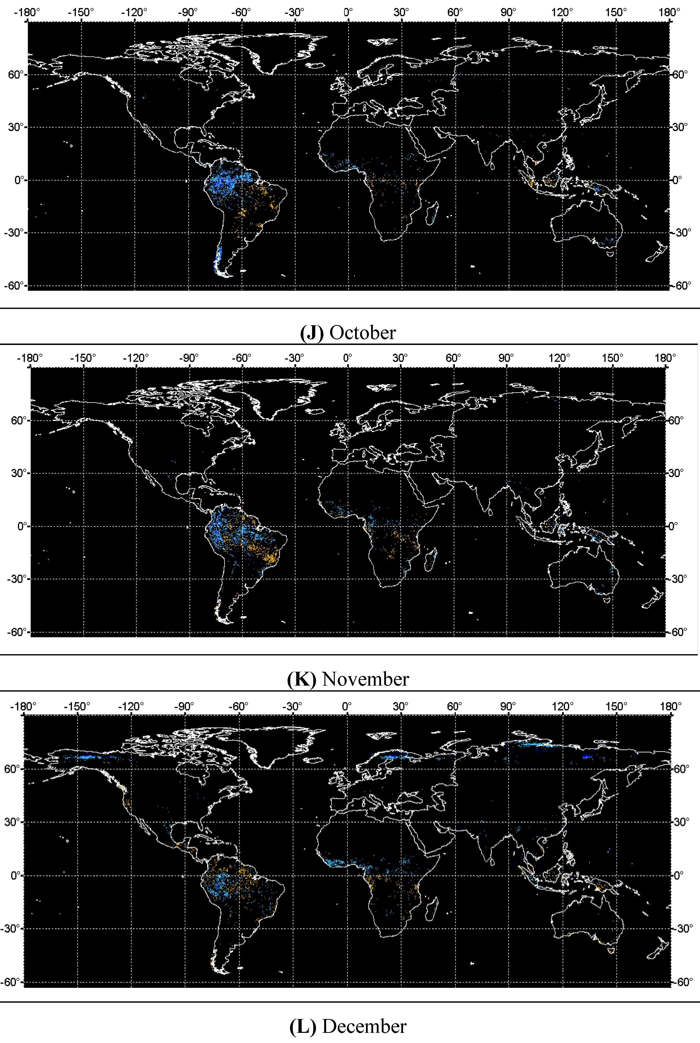
The monthly linear compositions of the first 10 principle components according to their eigenvalue percentage are listed in Figure 4 to show the dominating change tendency of NDVI anomaly values in period 1982–2006. Considering the uncertainties of time-series GIMMS data [41], changes between −0.05 and 0.05 are regarded as an unobvious change tendency, which is depicted in the figure by black. Otherwise, the change is regarded as obvious change tendency, which is shown in the figure by colors. For each month, the 10-PC composition can reflect the stable change trend during 1982–2006. It can reflect the global spatial distribution for each month. Meanwhile, comparison among months can reflect the temporal variation, showing a spatial pattern transfer between months. From Figure 4 and the aforementioned hypotheses, the stable monthly change tendency of global vegetation growth over the past two decades can be determined. The main profile of these change patterns is described as follows:
(1) The monthly change tendency of global vegetation growth shows obvious spatial heterogeneity.
The most obvious regions are embodied in the north middle or high latitudes, such as Siberia (see Figure 4(E) and (F)), northeastern China (see Figure 4(F)), western Alaska (see Figure 4(E,L)), eastern and northeastern Europe (see Figure 4(D,E,F)), as well as regions within or near the Tropic of Cancer and Capricorn (see Figure 4(A–L); such as central and northern parts of South America, central Africa, southern Africa, southeastern Australia, southern Asia, besides, southern and southwestern China.
(2) Change tendency between months also shows obvious global temporal heterogeneity over continental scale.
Eurasian Continent: In northeastern Europe (Figure 4(E)), central Siberia (Figure 4(E)), England and northwestern Europe (Figure 4(F)) and northeastern China (Figure 4(F)); strong positive phase signals appear in May or June, which are accompanied by an obvious rising tendency in vegetation activity. This indicates that the vegetation growth season in middle or high latitudes of Eurasian Continent feature signs of an earlier arrival with increasing vegetation vigor. In northern Siberia (Figure 4(F)), where the open-shrub grows [60], there is a negative phase in June, meaning decreasing vegetation vigor. In southern and southwestern China, obvious negative phase signals appear in July (Figure 4(G))—on the contrary, a positive phase emerges in August (Figure 4(H)). This development may have resulted from crop harvest and cycles in southern China during July–August [61]. In southeastern Asia, which is close to the Equator, vegetation vigor basically remains in a positive phase year round, except in September.
North America: In Alaska and northeastern Canada where open-shrub grows [60,62], there are negative phases in May and June (Figure 4(E) and (F)), revealing a possible delay to the start of the growth season. While in the continental United States, no obvious phase is found from the analysis.
South America: The northwestern areas of South America mainly feature a negative phase from September until the following May (Figure 4(A–E) and 4(I–L)) with an occasional positive phase in the eastern parts; an obvious positive phase appears from June to August (Figure 4(F–H)). This phenomenon shows that vegetation vigor in the northern South America region decreases during flourishing seasons. However, in non-flourishing seasons like June to August, vegetation activity shows signs of increasing. That is, vegetation vigor increases in winter and decreases during growth seasons.
Africa: the central region of Africa closest to the southern Sahara has a nearly negative phase over the course of an entire year (Figure 4), and is mainly characterized by open-shrub land [60]. This implies that drought area vegetation vigor has the tendency to decline under the environmental conditions of global warming. In the northern regions of Africa and around the Equator area, where woods grow [60], the NDVI change shows a positive phase in winter (Figure 4(F–H)), while in other seasons the NDVI change is primarily negative.
Australia: an obvious NDVI change phase is found primarily in the southeastern areas. A positive phase appears from January to April (Figure 4(A–D)), with increasing vegetation activity during the growth season. A negative phase appears from September to October (Figure 4(I–J)), with a decreasing tendency for vegetation activity during the non-flourishing season. No obvious vegetation activity tendency is found in other months.
Figure 4. The spatial patterns of the 10t ten principal components linear composition of monthly global NDVI anomaly transformation during 1982–2006 by EOF method, showing global vegetation total changing patterns and trends. The obvious change tendency is represented by the colors or in black.
Remotesensing 02 01530 g004aRemotesensing 02 01530 g004bRemotesensing 02 01530 g004cRemotesensing 02 01530 g004d
As stated above, vegetation growth vigor shows obvious spatial-temporal heterogeneity on a global scale. In the middle and high latitude areas of the north hemisphere, the difference among change tendencies is obvious in the time phase. This indicates that vegetation vigor change patterns have stronger heterogeneity in terms of tendency and are more complex. However, in central Siberia and northeastern China, there is a clear increasing tendency in May and June. In the land around the Arctic Ocean, the open-shrubs appear to have a decreasing tendency at the onset of the growth season. In the regions of Africa and South America within the Tropic of Cancer and Capricorn, vegetation changes almost always feature the same phase, including a shortened flourishing period, possibly attributed to certain global factors [11,63]. Meanwhile, in the southern hemisphere, vegetation activity during the non-flourishing period shows signs of an increase.

4. Discussions

In recent years, the fact that global warming is currently occurring has largely been accepted within the scientific community, and it has had an obvious impact on vegetation growth [64]. Many plants have changed their related activities when spring and autumn arrives in order to adapt to longer growing seasons created by global warming [15]. Additionally, vegetation activity has shown greater amplitude during seasonal changes [4]. However, the global warming trend has also featured clear heterogeneity on the global scale [65]. In some regions, the past few decades have shown a declining temperature trend, or less clear warming tendency [17,64]. A number of research studies have explored the spatial correlation between NDVI and climate variables [56,57,66], but different vegetation types show different responses to climate change [67]. Normally, vegetation activity is closely correlated to surface temperature [68]. However, the relationship between vegetation growth and temperature in low latitudes is relatively complex, where temperature does not inhibit vegetation growth [25]. Precipitation and carbon dioxide concentrations also affect vegetation growth [69,70]. There is a time lag for vegetation growth in response to precipitation [71]. This lag causes significant variation in regional vegetation’s sensitivity to precipitation—thus contributing to heterogeneity and complexity in the response of vegetation growth to global change. In addition, the spatio-temporal pattern of global vegetation growth is also influenced by large-scale regional climate oscillation [72,73]. For example, regions with obvious NDVI dynamic change have been found to have certain spatial connections to regions where vegetation is sensitive to the impact of North Atlantic Oscillation [74]. The connection between macro-climatic oscillation and regional vegetation activity can extend geographically to a global scope under certain laws.
Beyond climate change, land cover change and land use conversion also likely change the local or sub-regional NDVI. For instance, the tropical forest degradation caused by logging and burning leads to an obvious decreasing trend in temporal NDVI [75]. The logging in the mature forests of North America also caused a NDVI decrease in the 1990s [76]. Globally, the rate of deforestation has accelerated from the 1980s to the 1990s, especially in tropical Asia and Latin America [77]. On the other hand, forestation and regeneration could facilitate an increasing NDVI trend. For example, the “Grain for Green” Program launched in 1999 resulted in a significant increase of the forest cover in western China by planting trees and sowing grasses on steep slope agricultural cropland [78,79]. Partial disturbances such as forest rotation or farmland rotation generally cannot show an obvious stable NDVI change trend in the decade’s temporal scale, but the local plant habit change is an exception. For example, because improvements in hybrid rice breeding, the farmer’s practice of the three-crop per year thorough turned to two or one-crop a year in the past decade in southern China [80], which likely change the NDVI trend. However, for such local vegetation changes, only large-scale stable changes can be detected in this study by a coarse resolution time-series NDVI.
Most of results in this study support the conclusions of a variety of different reports of relevant regional to global research, while some inconsistencies can be found in local studies. For instance, middle and high latitude areas in the northern hemisphere have increased vegetation activity during growing seasons. Vegetation activity in low latitudes experiences a tendency for enlarged amplitude. However, quite different conclusions were drawn from some regional studies in the past, like on vegetation cover change in northwestern China. Ma et al. [81] analyzed 21-year NOAA/AVHRR NDVI images, ranging from 1981 to 2001, by using the EOS Pathfinder database and found that vegetation cover in northwestern China over the last 21 years is suffering a general degradation. Piao and Fang [82] also found that vegetation degradation primarily appeared in northwestern China and Qinghai-Tibet Plateau. However, other studies reported that over the past two decades, vegetation activity in the northern hemisphere and China was increasing, especially in the western part of China [83]. Most of these studies focused on vegetation changes on regional scales, but the results are controversial. Our finding in this paper is that the tendency of vegetation growth and variation in the frequent drought conditions of northwestern China and alpine regions is not obvious or it’s hard to detect, which is consistent with findings from other research on NDVI records concerning vegetation changes in the alpine regions along Yangtze and Yellow Rivers by using Pathfinder NOAA-AVHRR/NDVI time-series data [84]. Therefore, in areas with relatively low NDVIs, using time-series NDVI to analyze vegetation growth and variation on a regional scale, it still should be conducted carefully because of the disturbance from the soil background [85]. For instance, McCloy et al. [86] used three temporal NDVI datasets (Pathfinder, GIMMS and Fasir) to conduct a trend analysis, and found that the regional differences between the datasets are of such magnitude that these datasets cannot be used for regional mapping or monitoring. The other study on alpine grassland phenology using AVHRR, VEGETATION and MODIS NDVI also resulted in significant differences [87]. Though the AVHRR-NDVI has been used to analyze vegetation changes, including phenology, since early 1980s [88], greater numbers of similar studies have recently used finer resolution remotely sensed NDVI to conduct such an analysis. 250 m, 500 m and 1 km MODIS and VEGETATION NDVI are the most frequently used data to retrieve and monitor the global vegetation phenology [89,90,91]. Research on regional vegetation growth and its variation should consider the impact of the data spatial scale. In order to improve accuracy, future studies need to use remotely sensed data with a finer spatial resolution, or combine the data with field observations. Moreover, studies should take into consideration the impact of NDVI sensitivity on low vegetation cover in bare areas. However, though the AVHRR NDVI dataset with 8 km resolution has some limitations as described above, it is still applicable in studying global change issues, because of its reliable, extended history of more than 20 years.

5. Conclusions

GIMMS-NDVI time-series data are applied to analyze global vegetation vigor dynamics in this paper. The empirical orthogonal function (EOF) is used to extract the phase changes of the NDVI from a long sequence cycle from the 25 year period of 1982–2006, and the monthly NDVI change phase is connected to the specific vegetation activities. Spatial-temporal change patterns are summarized.
Change in global vegetation vigor has a high spatial-temporal heterogeneity. Regions with the most obvious monthly change trend are distributed geographically at the middle and high latitude of north hemisphere, including northeastern Europe, Siberia, northeastern China, and regions within or near the Tropic of Cancer and Capricorn; like southern and southwestern China, northwestern parts of South America, central and southern Africa, and southeastern Australia. Over the last two decades, the inter-annual spatial and phase transfer of global vegetation growth seasons show obvious laws. In middle and high latitude areas of the northern hemisphere, the phases of vegetation activity are more positive in growth seasons, revealing signs that the vegetation growth season is increasing in duration. In low latitude areas, vegetation activities decrease in flourishing seasons, while they increase in non-flourishing seasons.
A wealth of research shows that the regional climate change caused by global warming is a leading factor influencing vegetation growth and change tendencies on a global scale over the past two decades. This tendency can also be influenced by vegetation type and regional climate oscillation on macro scales. Our analysis strongly supports a variety of different reports in existing literature, such as earlier growing seasons at higher northern latitudes, which is directly linked to increasing surface temperatures. However, investigating vegetation activity in those regions like drought and alpine, should be fully cautious when using NDVI time-series datasets.

Acknowledgements

The authors wish to express their gratitude to the NASA Global Inventory Modeling and Mapping Studies (GIMMS) group for the AVHRR GIMMS NDVI dataset. This work was supported partly by the Western Light Talent Culture project (No. O8R2130130), the Knowledge Innovation Program of the Chinese Academy of Sciences (Grant No. KZCX2-YW-QN313), the State Key Development Program for Basic Research of China (Grant No. 2006CB403301), and a NASA grant. We are grateful to the anonymous reviewers for their comments.

References

  1. Walker, B.H. Landscape to regional-scale responses of terrestrial ecosystems to global change. Ambio 1994, 23, 67–73. [Google Scholar]
  2. Friedlingstin, P.; Dufrene, J.-L.; Cox, P.M.; Rayner, P. How positive is the feedback between climate change and the carbon cycle? Tellus 2003, 55B, 692–700. [Google Scholar] [CrossRef]
  3. Houghton, J.T.; Ding, Y.; Griggs, D.J.; Noguer, M.; van der Linden, P.J.; Xiaosu, D. Climate Change 2001: The Scientific Basis Contribution of Working Group I to the Third Assessment Report of the Intergovernmental Panel on Climate Change (IPCC); Cambridge University Press: Cambridge, UK, 2001. [Google Scholar]
  4. Fang, X.Q.; Yu, W.H. Progress in the studies on the phenological responding to globalwarming. Adv. Earth Sci. 2002, 17, 714–719. [Google Scholar]
  5. Houghton, J.T. Counting terrestrial sources and sinks of carbon. Climatic Change 2001, 48, 525–534. [Google Scholar] [CrossRef]
  6. Gurney, K.; Law, R.M.; Ddenning, A.S.; Rayner, P.J.; Baker, D.; Bousquet, P.; Bruhwiler, L.; Chen, Y.-H.; Ciais, P.; Fan, S.; Fung, I.Y.; Gloor, M.; Heimann, M.; Higuchi, K.; John, J.; Maki, T.; Maksyutov, S.; Masarie, K.; Peylin, P.; Prather, M.; Pak, B.C.; Randerson, J.; Sarmiento, J.; Taguchi, S.; Takahashi, T.; Yuen, C.-W. Towards robust regional estimates of CO2 sources and sinks using atmospheric transport models. Nature 2002, 415, 626–630. [Google Scholar] [CrossRef] [PubMed]
  7. Goulden, M.L.; Munger, J.W.; Fan, S.M.; Daube, B.C.; Wofsy, S.C. Exchange of carbon dioxide by a deciduous forest: Response to interannual climate variability. Science 1996, 271, 1576–1578. [Google Scholar] [CrossRef]
  8. Fang, J.Y.; Chen, A.; Peng, C.; Zhao, S.; Ci, L. Changes in forest biomass carbon storage in China between 1949 and 1998. Science 2001, 292, 2320–2322. [Google Scholar] [CrossRef] [PubMed]
  9. Fan, S.; Gloor, M.; Mahlman, J.; Pacala, S.; Sarmiento, J.; Takahashi, T.; Tans, P. A large terrestrial carbon sink in North America implied by atmospheric and oceanic carbon dioxide data and models. Science 1998, 282, 442–446. [Google Scholar] [CrossRef] [PubMed]
  10. Pacala, S.; Hurtt, G.C.; Baker, D.; Peylin, P.; Houghton, R.A.; Birdsey, R.A.; Health, L.; Sundquist, E.T.; Stallard, R.F.; Ciais, P.; Moorcroft, P.; Caspersen, J.; Shevliakova, E.; Moore, B.; Kohlmaier, G.; Holland, E.; Gloor, M.; Harmon, M.E.; Fan, S.M.; Sarmiento, J.L.; Goodale, C.L.; Schimel, D.; Field, C.B. Consistent land-and atmosphere-based US carbon sink estimates. Science 2001, 292, 2316–2319. [Google Scholar] [CrossRef] [PubMed]
  11. Foley, J.A.; Levis, S.; Costa, M.H.; Cramer, W.; Pollard, D. Incorporating dynamic vegetation cover within global climate models. Ecol. Appl. 2000, 10, 1620–1632. [Google Scholar] [CrossRef]
  12. Bogaert, J.; Zhou, L.; Tucker, C.J. Evidence for a persistent and extensive greening trend in Eurasia inferred from satellite vegetation index data. J. Geophys. Res. 2002, 107, 4119–4135. [Google Scholar] [CrossRef]
  13. Zhou, L.; Tucker, C.J.; Kaufmann, R.K. Variations in northern vegetation activity inferred from satellite data of vegetation index during 1981 to 1999. J. Geophys. Res. 2001, 106, 20069–20083. [Google Scholar] [CrossRef]
  14. Burkett, V.R.; Wilcox, D.A.; Stottlemyer, R.; Barrow, W.; Fagre, D.; Baron, J.; Price, J.; Nielsen, J.L.; Allen, C.D.; Peterson, D.L.; Ruggerone, G.; Doyle, T. Nonlinear dynamics in ecosystem response to climatic change: Case studies and policy implications. Ecol. Complex. 2005, 2, 357–394. [Google Scholar] [CrossRef]
  15. Keeling, C.D.; Chin, J.F.S.; Whorf, T.P. Incressed activity of northern vegetation in inferred from atmospheric CO2 measurements. Nature 1996, 382, 146–149. [Google Scholar] [CrossRef]
  16. Menzel, A. Phenology: Its importance to the global change community. Climate Change 2002, 54, 379–395. [Google Scholar] [CrossRef]
  17. IPCC. Climate Change 2007: Synthesis Report; Cambridge University Press: Cambridge, UK; New York, NY, USA, 2007. [Google Scholar]
  18. Tucker, C.J. Red and photographic infrared linear combinations for monitoring vegetation. Remote Sens. Environ. 1979, 8, 127–150. [Google Scholar] [CrossRef]
  19. Liang, S. Quantitative Remote Sensing of Land Surfaces; John Wiley & Sons: Hoboken, NJ, USA, 2004. [Google Scholar]
  20. Myneni, R.B.; Hall, F.G.; Sellers, P.J.; Marshak, A.L. The interpretation of spectral vegetation indexes. IEEE Trans. Geosci. Remot. Sens. 1995, 33, 481–486. [Google Scholar] [CrossRef]
  21. Tucker, C.J.; Fung, I.Y.; Hall, C.D. Relationship between atmospheric CO2 variations and a satellite-derived vegetation index. Nature 1986, 319, 195–199. [Google Scholar] [CrossRef]
  22. Holben, B.N. Characteristics of maximum-value composite images from Temporal AVHRR Data. Int. J. Remote Sens. 1986, 7, 1417–1434. [Google Scholar] [CrossRef]
  23. Li, A.; Liang, S.; Wang, A.; Qin, J. Estimating crop yield from multi-temporal satellite data using multivariate regression and neural network techniques. Photogramm. Eng. Remote Sensing 2007, 73, 1149–1159. [Google Scholar] [CrossRef]
  24. Doktor, D.; Bondeau, A.; Koslowski, D.; Badeck, F.-W. Influence of heterogeneous landscapes on computed green-up dates based on daily AVHRR NDVI observations. Remote Sens. Environ. 2009, 113, 2618–2632. [Google Scholar] [CrossRef]
  25. Bajgiran, P.R.; Darvishsefat, A.A.; Khalili, A.; Makhdoum, M.F. Using AVHRR-based vegetation indices for drought monitoring in the northwest of Iran. J. Arid Environ. 2008, 72, 1086–1096. [Google Scholar] [CrossRef]
  26. Paruelo, J.M.; Aguiar, M.R.; Golluscio, R.A.; Leon, R.J.C.; Pujol, G. Environmental controls of NDVI dynamics in patagonia based on noaa-avhrr satellite data. J. Veg. Sci. 1993, 4, 425–428. [Google Scholar] [CrossRef]
  27. de Beurs, K.M.; Henebry, G.M. A statistical framework for the analysis of long image time-series. Int. J. Remote Sens. 2005, 26, 1551–1573. [Google Scholar] [CrossRef]
  28. Bradley, B.A.; Jacob, R.W.; Hermance, J.F.; Mustard, J.F. A curve fitting procedure to derive inter-annual phenologies from time-series of noisy satellite NDVI data. Remote Sens. Environ. 2007, 106, 137–145. [Google Scholar] [CrossRef]
  29. Walker, B.; Steffen, W. An overview of the implications of global change for natural and managed terrestrial ecosystems. Conserv. Ecol. 1997, 1. Available online: http://www.ecologyandsociety.org/vol1/iss2/art2/ (accessed on 20 April 2010). [Google Scholar]
  30. Eastman, J.R.; Fulk, M. Long sequence time-series evaluation using standardized principal components. Photogramm. Eng. Remote Sensing 1993, 59, 991–996. [Google Scholar]
  31. Townshed, J.R.G.; Goff, T.E.; Tucker, C.J. Multitemporal dimensionality of images of Normalized Difference Vegetation Index at continental scales. IEEE Trans. Geosci. Remot. Sen. 1985, GE-23, 888–895. [Google Scholar] [CrossRef]
  32. Jönsson, P.; Eklundh, L. TIMESAT—A program for analyzing time-series of satellite sensor data. Comput. Geosci. 2004, 30, 833–845. [Google Scholar] [CrossRef]
  33. Azzali, A.; Menenti, M. Mapping vegetation—Soil complexes in southern Africa using temporal Fourier analysis of NOAA AVHRR NDVI data. Int. J. Remote Sens. 2000, 21, 973–996. [Google Scholar] [CrossRef]
  34. Jakubauskas, M.E.; Legates, D.R.; Kastens, J.H. Harmonic analysis of time-series AVHRR NDVI data. Photogramm. Eng. Remote Sensing 2001, 67, 461–470. [Google Scholar]
  35. Galford, G.L.; Mustard, J.F.; Melillo, J.; Gendrin, A.; Cerri, C.C.; Cerri, C.E.P. Wavelet analysis of MODIS time-series to detect expansion and intensification of row-crop agriculture in Brazil. Remote Sensi. Environ. 2008, 112, 576–587. [Google Scholar] [CrossRef]
  36. Martínez, B.; Gilabert, M.A. Vegetation dynamics from NDVI time-series analysis using the wavelet transform. Remote Sensi. Environ. 2009, 113, 1823–1842. [Google Scholar] [CrossRef]
  37. Suzuki, R.; Masuda, K.; Dye, D.G. Interannual covariability between actual evapotranspiration and PAL and GIMMS NDVIs of northern Asia. Remote Sensi. Environ. 2007, 106, 387–398. [Google Scholar] [CrossRef]
  38. Heumann, B.W.; Seaquist, J.W.; Eklundh, L.; Jönsson, P. AVHRR derived phenological change in the Sahel and Soudan, Africa, 1982–2005. Remote Sensi. Environ. 2007, 108, 385–392. [Google Scholar] [CrossRef]
  39. Slayback, D.A.; Pinzon, J.E.; Los, S.O. Northern hemisphere photosynthetic trends 1982–99. Glob. Change Biol. 2003, 9, 1–15. [Google Scholar] [CrossRef]
  40. Davenport, M.L.; Nicholson, S.E. On the Relation between rainfall and the Normalized Difference Vegetation Index for diverse vegetation types in East Africa. Int. J. Remote Sens. 1993, 14, 2369–2389. [Google Scholar] [CrossRef]
  41. Fensholt, R.; Rasmussen, K.; Nielsen, T.T.; Mbow, C. Evaluation of earth observation based long term vegetation trends—Intercomparing NDVI time-series trend analysis consistency of Sahel from AVHRR GIMMS, Terra MODIS and SPOT VGT data. Remote Sens. Environ. 2009, 113, 1886–1898. [Google Scholar] [CrossRef]
  42. Tucker, C.J.; Pinzon, J.E.; Brown, M.E.; Slayback, D.A.; Pak, E.W.; Mahoney, R.; Vermote, E.F.; El Saleous, N. An extended AVHRR 8-km NDVI dataset compatible with MODIS and SPOT vegetation NDVI data. Int. J. Remote Sens. 2005, 26, 4485–4498. [Google Scholar] [CrossRef]
  43. Cihlar, J.; Chen, J.; Li, Z.; Huang, F.; Pokrant, H. Can interannual land surface signal be discerned in composite AVHRR data? J. Geophys. Res. 1998, 103, 23163–23172. [Google Scholar] [CrossRef]
  44. Nagol, J.R.; Vermote, E.F.; Prince, S.D. Effects of atmospheric variation on AVHRR NDVI data. Remote Sens. Environ. 2009, 113, 392–397. [Google Scholar] [CrossRef]
  45. Diwakar, P.G.; Prabhakar, P.; Venkataramana, I.; Devarajan, R. Derivation of maximum value composite images using multidate NOAA-AVHRR data. J. Indian Soc. Remote Sens. 1989, 17, 1–6. [Google Scholar] [CrossRef]
  46. Savitzky, A.; Golay, M.J.E. Smoothing and differentiation of data by simplified least squares procedures. Anal. Chem. 1964, 36, 1627–1639. [Google Scholar] [CrossRef]
  47. Chen, J.; Jönsson, P.; Tamura, M.; Gu, Z.; Matsushita, B.; Eklundh, L. A simple method for reconstructing a high-quality NDVI time-series data set based on the Savitzky–Golay filter. Remote Sens. Environ. 2004, 91, 332–344. [Google Scholar] [CrossRef]
  48. Bian, J.; Li, A.; Song, M.; Ma, L.; Jiang, J. Reconstructing NDVI time-series data set based on the Savitzky-Golay filter. J. Remote Sens. 2010, 14, 001–009. [Google Scholar]
  49. Steinier, J.; Termonia, Y.; Deltour, J. Comments on smoothing and differentiation of data by simplified least squares procedure. Anal. Chem. 1972, 44, 1906–1909. [Google Scholar] [CrossRef] [PubMed]
  50. Richardson, A.J.; Wiegand, C.L. Distinguishing vegetation from soil background information. Photogramm. Eng. Remote Sensing 1977, 43, 1541–1552. [Google Scholar]
  51. Hannachi, A.; Unkel, S.; Trendafilov, N.T.; Jolliffe, I.T. Independent component analysis of climate data: A new look at EOF rotation. J. Climate 2009, 22, 2797–2812. [Google Scholar] [CrossRef]
  52. Obukhov, A.M. Statistically homogeneous fields on a sphere. Uspekhi Matematicheskikh Nauk 1947, 2, 196–198. [Google Scholar]
  53. Carleton, A.M. Methodology in climatology. Ann. Assn. Amer. Geogr. 1999, 89, 713–735. [Google Scholar] [CrossRef]
  54. Jolliffe, I.T. Principal Component Analysis; Springer: Berlin, Germany, 2002. [Google Scholar]
  55. Prasad, A.K.; Sarkar, S.; Singh, R.P.; Kafatos, M. Inter-annual variability of vegetation cover and rainfall over india. Adv. Space Res. 2007, 39, 79–87. [Google Scholar] [CrossRef]
  56. Nezlin, N.P.; Kostianoy, A.G.; Li, B.-L. Inter-annual variability and interaction of remote-sensed vegetation index and atmospheric precipitation in the Aral Sea region. J. Arid Environ. 2005, 62, 677–700. [Google Scholar] [CrossRef]
  57. Sarkar, S.; Kafatos, M. Interannual variability of vegetation over the Indian sub-continent and its relation to the different meteorological parameters. Remote Sens. Environ. 2004, 90, 268–280. [Google Scholar] [CrossRef]
  58. Lobo, A.; Maisongrande, P. Searching for trends of change through exploratory data analysis of time-series of remotely sensed images of SW Europe and NW Africa. Int. J. Remote Sens. 2008, 29, 5237–5245. [Google Scholar] [CrossRef]
  59. Golub, G.H.; van Loan, C.F. Matrix Computations; The John Hopkins University Press: Baltimore, MD, USA, 1996. [Google Scholar]
  60. Hansen, M.; DeFries, R.; Townshend, J.R.G.; Sohlberg, R. Global land cover classification at 1km resolution using a decision tree classifier. Int. J. Remote Sens. 2000, 21, 1331–1365. [Google Scholar] [CrossRef]
  61. Huang, Y.; Zhang, W.; Sun, W.; Zheng, X. Net primary production of Chinese croplands from 1950 to 1999. Ecol. Appl. 2007, 17, 692–701. [Google Scholar] [CrossRef] [PubMed]
  62. Jia, G.J.; Epstein, H.E.; Walker, D.A. Spatial characteristics of AVHRR-NDVI along latitudinal transects in northern Alaska. J. Veg. Sci. 2002, 13, 315–326. [Google Scholar] [CrossRef]
  63. Dewar, R.C.; Franklin, O.; Mäkelä, A.; Mcmurtrie, R.E.; Valentine, H.T. Optimal Function Explains Forest Responses to Global Change. BioScience 2009, 59, 127–139. [Google Scholar] [CrossRef]
  64. IPCC. Climate Change 2001: The Science of Climate Change; Contribution of Working Group I to the Third Assessment Report of the Intergovernmental Panel on Climate Change; Cambridge University Press: Cambridge, UK, 2001; p. 658. [Google Scholar]
  65. Hansen, J.; Sato, M.; Ruedy, R.; Lo, K.; Lea, D.W.; Medina-Elizade, M. Global temperature change. PNAS 2006, 103, 14288–14293. [Google Scholar] [CrossRef] [PubMed]
  66. Kawabata, A.; Yamaguchi, Y. Global monitoring of interannnual changes in vegetation activities using NDVI and its relationships to temperature and precipitation. Int. J. Remote Sens. 2001, 22, 1377–1382. [Google Scholar] [CrossRef]
  67. Piao, S.L.; Fang, J.Y.; Chen, A.P. Seasonal dynamics of terrestrial primary production in response to climate change in China. Acta Bot. Sin. 2003, 45, 269–275. [Google Scholar]
  68. Notaro, M. Response of the mean global vegetation distribution to interannual climate variability. Clim. Dynam. 2008, 30, 845–854. [Google Scholar] [CrossRef]
  69. Lotsch, A.; Friedl, M.A.; Anderson, B.T.; Tucker, C.J. Coupled vegetation-precipitation variability observed from satellite and climate records. Geophys. Res. Lett. 2003, 30, 1774. [Google Scholar] [CrossRef]
  70. Nemani, R.; White, M.; Thornton, P.; Nishida, K.; Reddy, S.; Jenkins, J.; Running, S. Recent trends in hydrologic balance have enhanced the terrestrial carbon sink in the United States. Geophys. Res. Lett. 2002, 29, 1468. [Google Scholar] [CrossRef]
  71. Shigehara, K. Phonological observation data in Japan to be utilized as an indicator of climatic variation. In Proceedings of the International Conference on Climatic Impacts on the Environment and Society; University of Tsukuba: Ibaraki, Japan, 1991; pp. C1–C6. [Google Scholar]
  72. Poveda, G.; Salazar, L.F. Annual and interannual (ENSO) variability of spatial scaling properties of a vegetation index (NDVI) in Amazonia. Remote Sens. Environ. 2004, 93, 391–401. [Google Scholar] [CrossRef]
  73. Ottersen, G.; Planque, B.; Belgravio, A. Ecological effects of the Northern Atlantic Oscillation. Oecologia 2001, 128, 1–14. [Google Scholar] [CrossRef]
  74. Li, A.; Liang, S.; Huang, C.; Wang, A. Investigating the impacts of the north Atlantic Oscillation on global vegetation changes. J. Geophys. Res. submitted.
  75. Souza, C.M.; Roberts, D.A.; Monteiro, A.L. Multitemporal analysis of degraded forests in the southern Brazilian Amazon. Earth Interactions 2005, 9, 1–25. [Google Scholar] [CrossRef]
  76. Potter, C.; Tan, P. N.; Kumar, V.; Kucharik, C.; Klooster, S.; Genovese, V.; Cohen, W.; Healey, S. Recent history of large-scale ecosystem disturbances in North America derived from the AVHRR satellite record. Ecosystems 2005, 8, 808–824. [Google Scholar] [CrossRef]
  77. Hansen, M.C.; DeFries, R.S. Detecting long-term global forest change using continuous fields of tree-cover maps from 8-km advanced very high resolution radiometer (AVHRR) data for the years 1982–99. Ecosystems 2004, 7, 695–716. [Google Scholar] [CrossRef]
  78. Zhou, H.J.; Van Rompaey, A.; Wang, J.A. Detecting the impact of the “Grain for Green” program on the mean annual vegetation cover in the Shaanxi province, China using SPOT-VGT NDVI data. Land Use Policy 2009, 26, 954–960. [Google Scholar] [CrossRef]
  79. Chen, X.G.; Zhang, X.Q.; Zhang, Y.P.; Wan, C.B. Carbon sequestration potential of the stands under the grain for green program in Yunnan province, China. Forest Ecol. Manage. 2009, 258, 199–206. [Google Scholar] [CrossRef]
  80. Erda, L. Agricultural vulnerability and adaptation to global, warming in China. Water Air Soil Pollut. 1996, 92, 63–73. [Google Scholar]
  81. Ma, M.G.; Dong, L.X.; Wang, X.M. Study on the dynamically monitoring and simulating the vegetation cover in northwest China in the past 21 years. J. Glaciol. Geocryol. 2003, 25, 232–236. [Google Scholar]
  82. Piao, S.L.; Fang, J.Y. Dynamic vegetation cover change over the last 18 years in China. Quaternary Sci. 2001, 21, 294–302. [Google Scholar]
  83. Cao, M.K.; Prince, S.D.; Li, K.P. Response of terrestrial carbon uptake to climate interannual variability in China. Glob. Change Biol. 2003, 9, 536–546. [Google Scholar] [CrossRef]
  84. Yang, J.P.; Ding, Y.J.; Chen, R.S. NDVI reflection of alpine vegetation changes in the source regions of the Yangtze and Yellow rivers. Acta Geographica Sinica 2005, 60, 467–478. [Google Scholar]
  85. Huete, A.R. A soil-adjusted vegetation index (SAVI). Remote Sens. Environ. 1988, 25, 53–70. [Google Scholar] [CrossRef]
  86. McCloy, K.R.; Los, S.; Lucht, W.; Højsgaard, S. A comparative analysis of three long-term NDVI datasets derived from AVHRR satellite data. EARSeL eProceedings 2005, 4, 52–69. [Google Scholar]
  87. Fontana, F.; Rixen, C.; Jonas, T.; Aberegg, G.; Wunderle, S. Alpine grassland phenology as seen in AVHRR, VEGETATION, and MODIS NDVI time-series—A comparison with in situ measurements. Sensors 2008, 8, 2833–2853. [Google Scholar] [CrossRef] [Green Version]
  88. Justice, C.O.; Townshend, J.R.G.; Holben, B.N.; Tucker, C.J. Analysis of the phenology of global vegetation using meteorological satellite data. Int. J. Remote Sens. 1985, 6, 1271–1318. [Google Scholar] [CrossRef]
  89. Knight, J.F.; Lunetta, R.S.; Ediriwickrema, J.; Khorrarn, S. Regional scale land cover characterization using MODIS-NDVI 250 m multi-temporal imagery: A phenology-based approach. GISci. Remote Sens. 2006, 43, 1–23. [Google Scholar] [CrossRef]
  90. van Leeuwen, W.J.D.; Davison, J.E.; Casady, G.M.; Marsh, S.E. Phenological characterization of desert sky island vegetation communities with remotely sensed and climate time-series data. Remote Sensing 2010, 2, 388–415. [Google Scholar] [CrossRef]
  91. Gu, Y.; Brown, J.F.; Miura, T.; van Leeuwen, W.J.D.; Reed, B.C. Phenological classification of the United States: A geographic framework for extending multi-sensor time-series data. Remote Sensing 2010, 2, 526–544. [Google Scholar] [CrossRef]