Geostatistics for Mapping Leaf Area Index over a Cropland Landscape: Efficiency Sampling Assessment


Abstract
:1. Introduction
2. Background
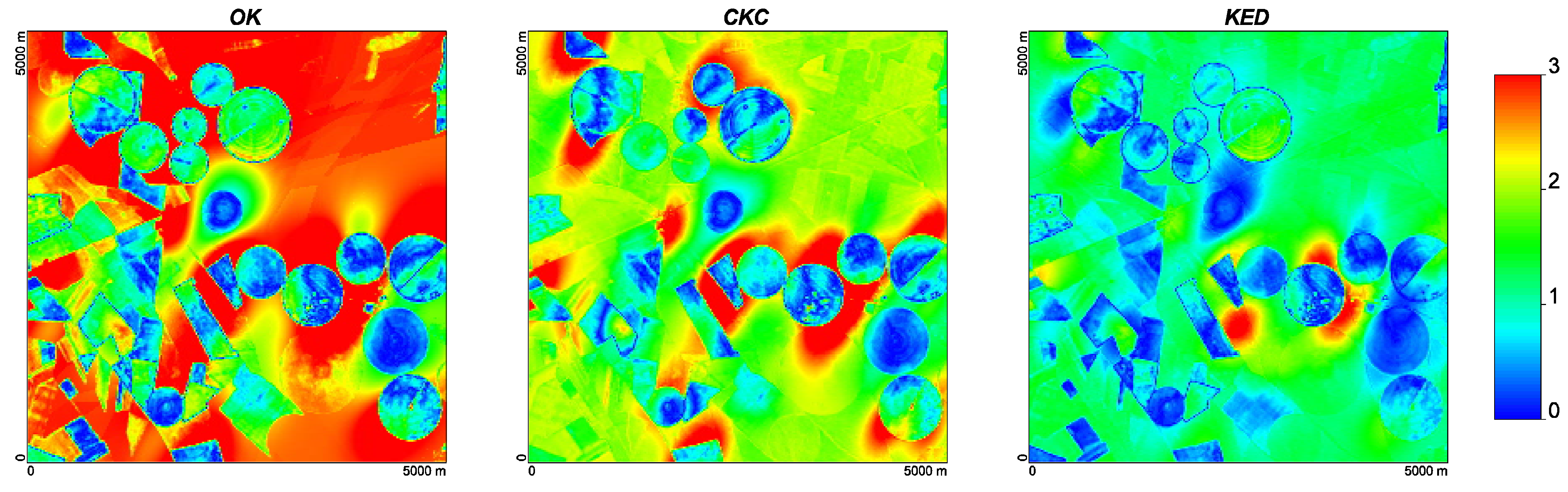
2.1. Ordinary Kriging (OK)
2.2. Kriging with an External Drift (KED)
2.3. Collocated Cokriging (CKC)

| Model trend | Non-Stationarity | Secondary variable | |
| OK | Unknown local mean m1(u) | No | No |
| CKC | Unknown local mean m1(u) | Yes | Yes |
| KED | Yes | Yes |
3. Methods
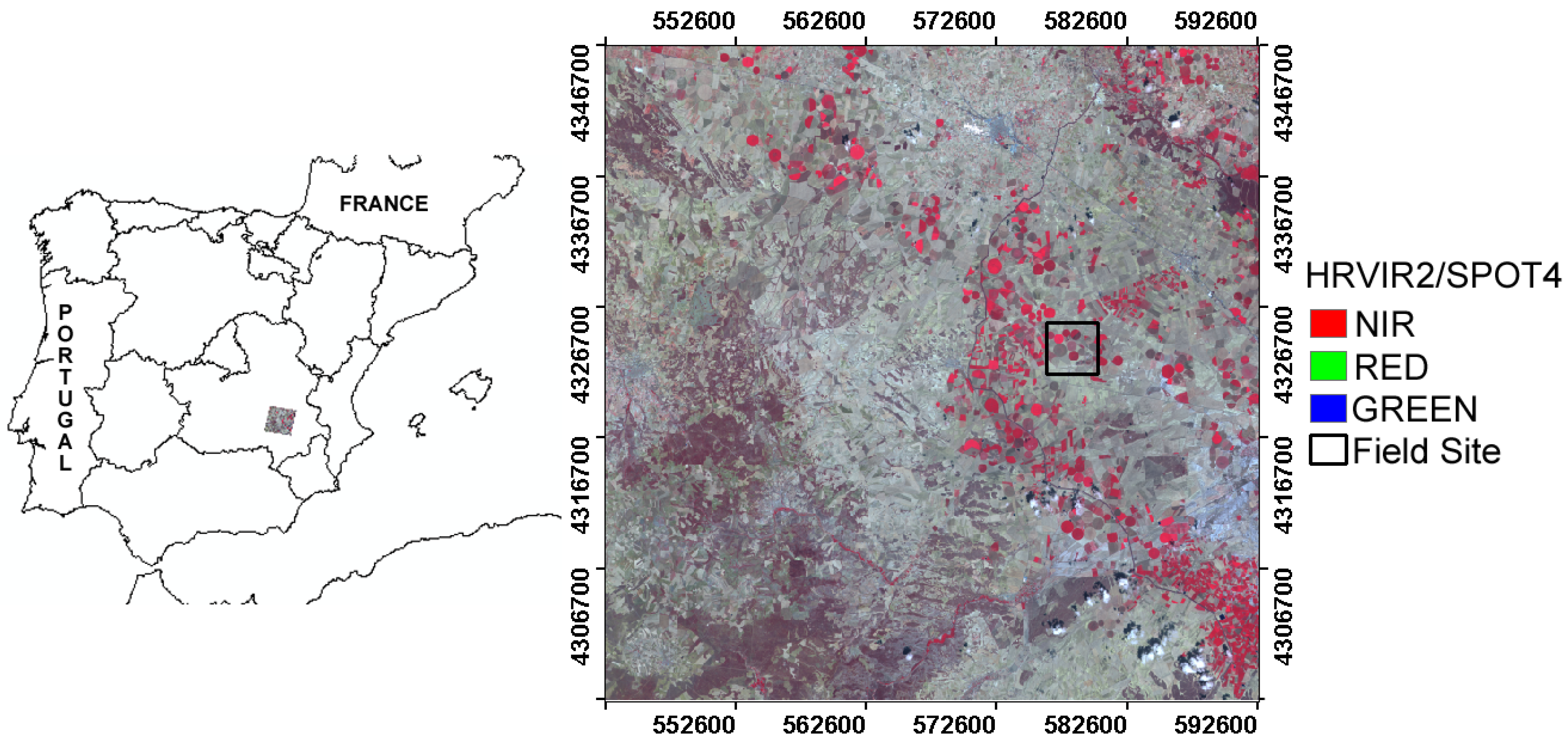
3.1. Study Area
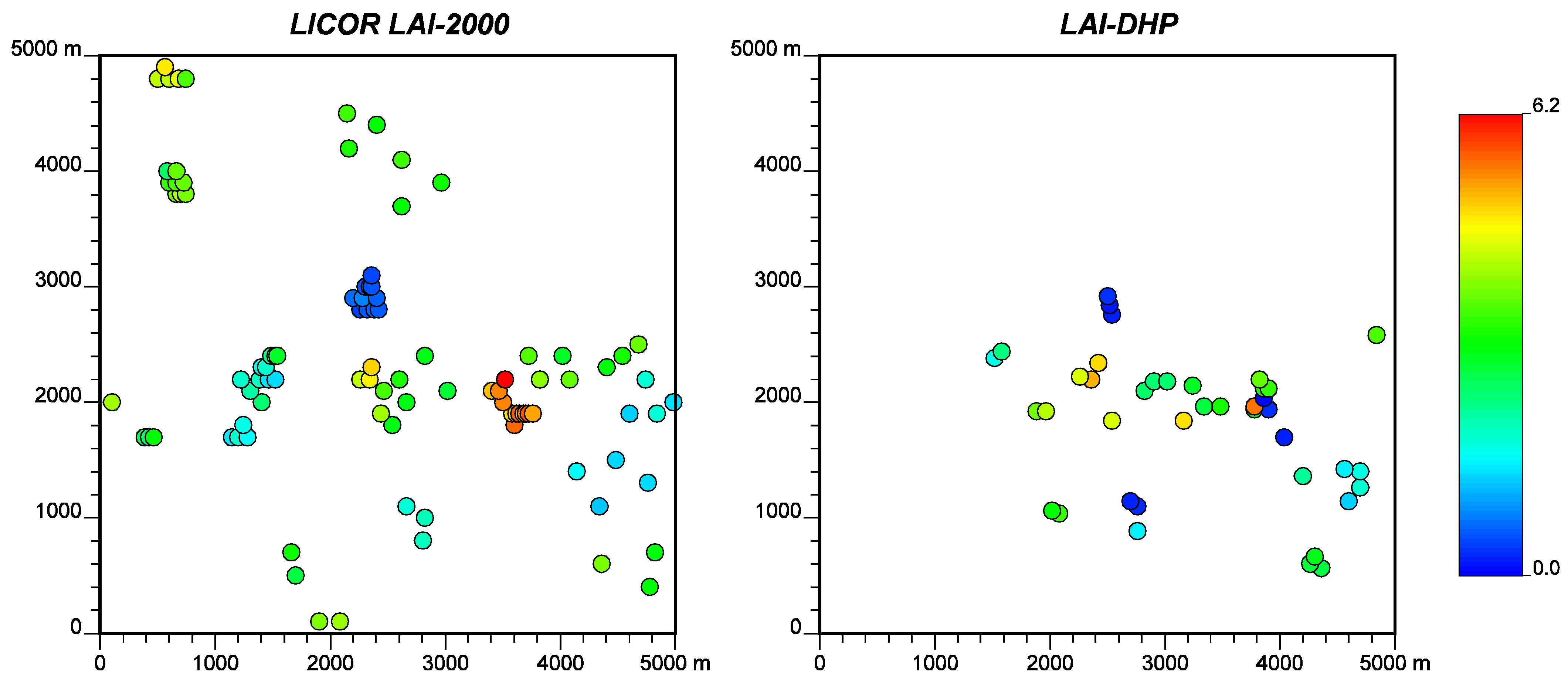
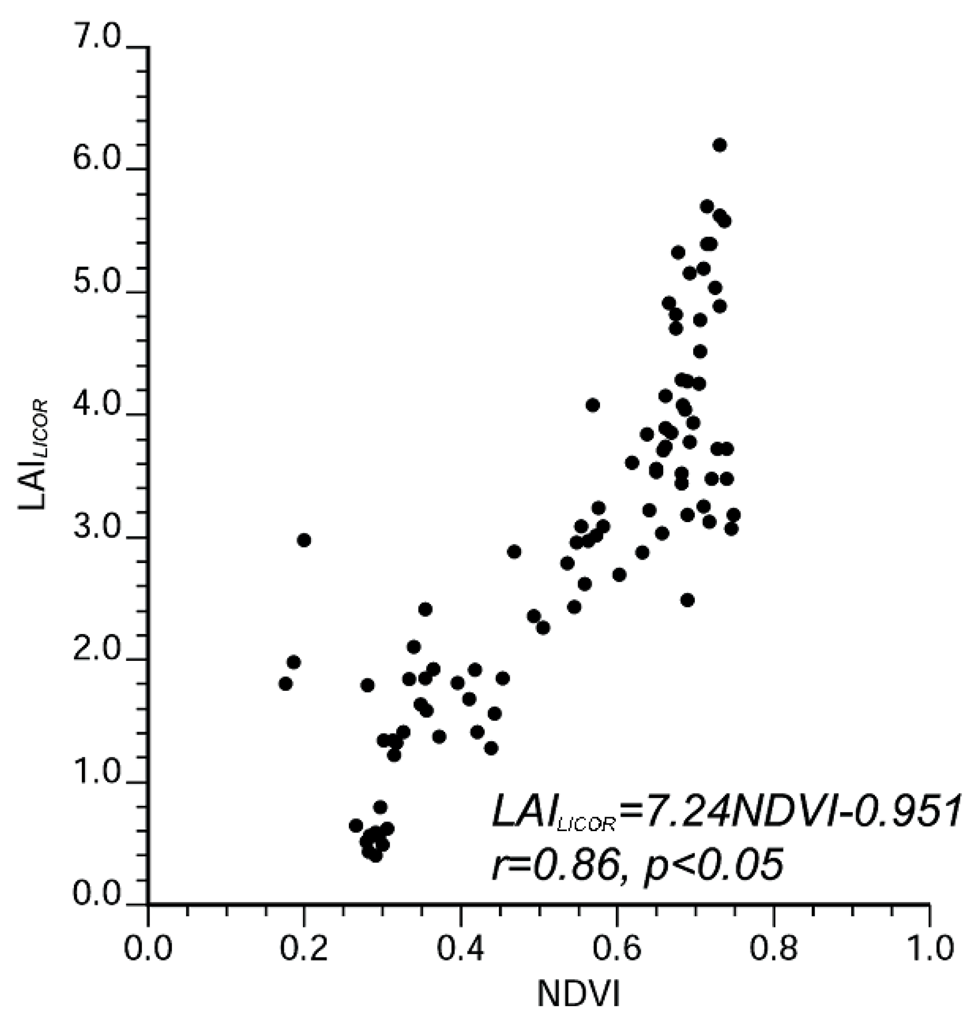
3.2. Field Measurements
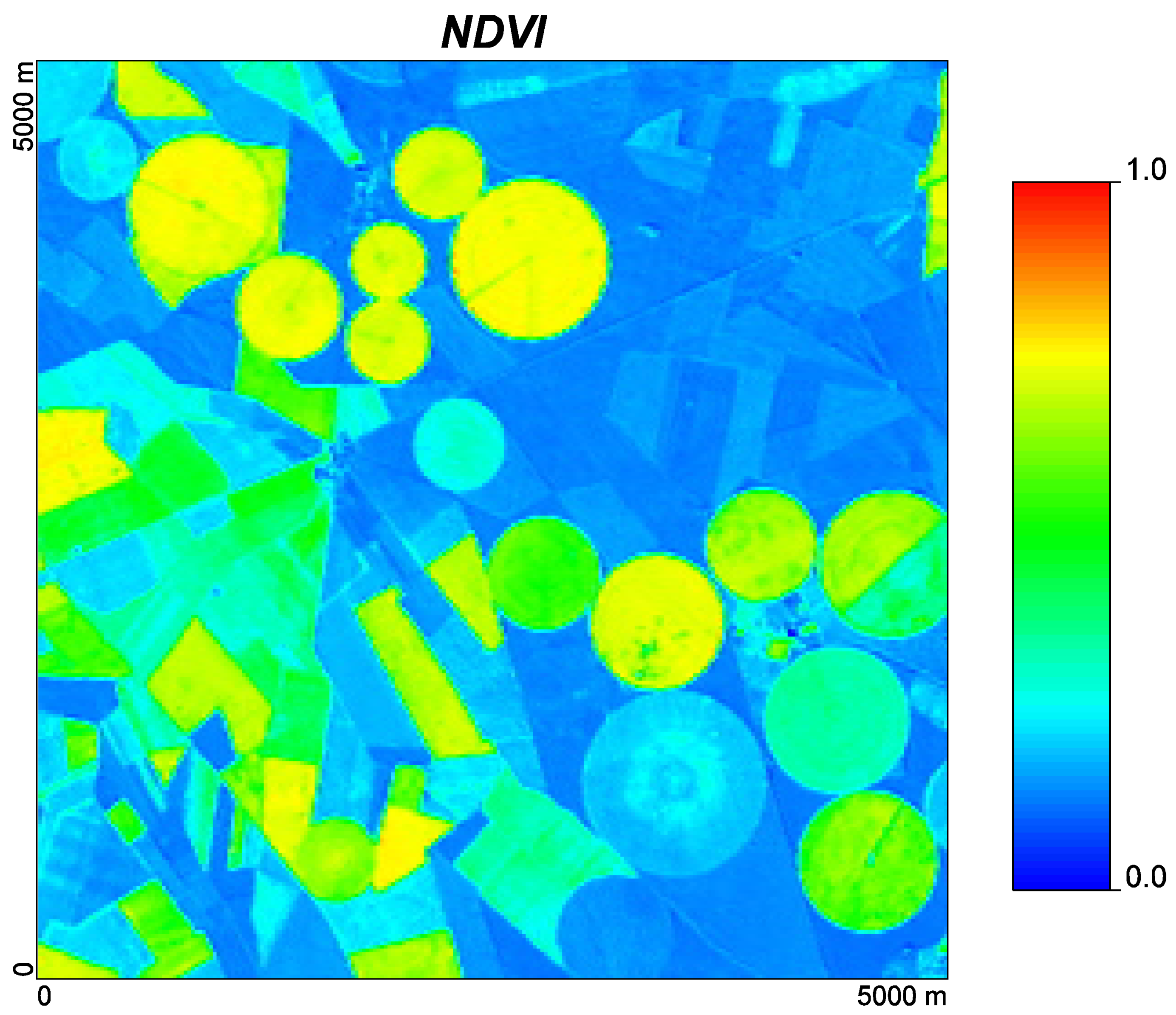
3.3. Auxiliary Information

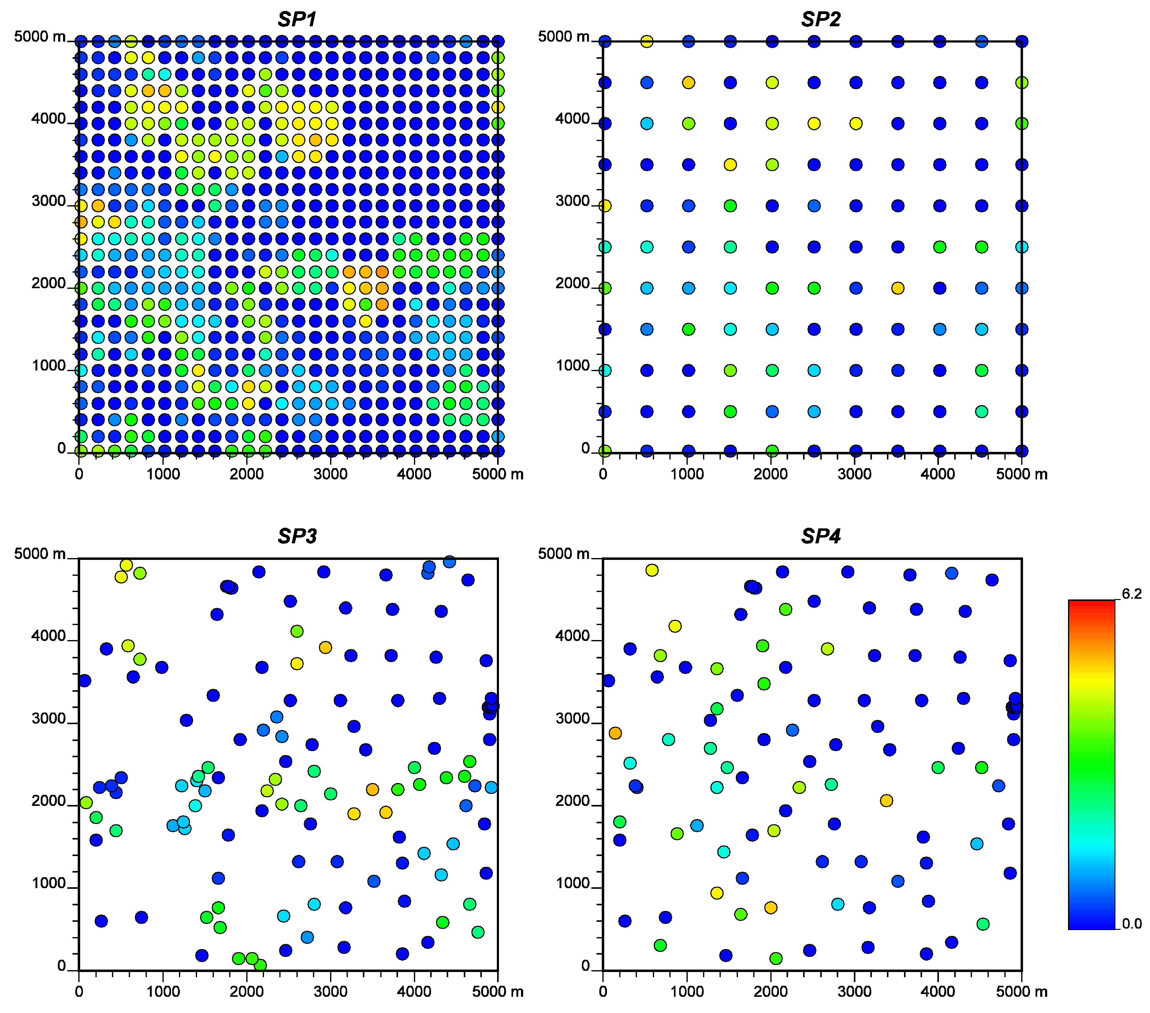
3.4. Sampling Strategy

3.5. LAI Predictions from OK, CKC and KED Models
3.6. LAI Predictions Assessment
4. Results
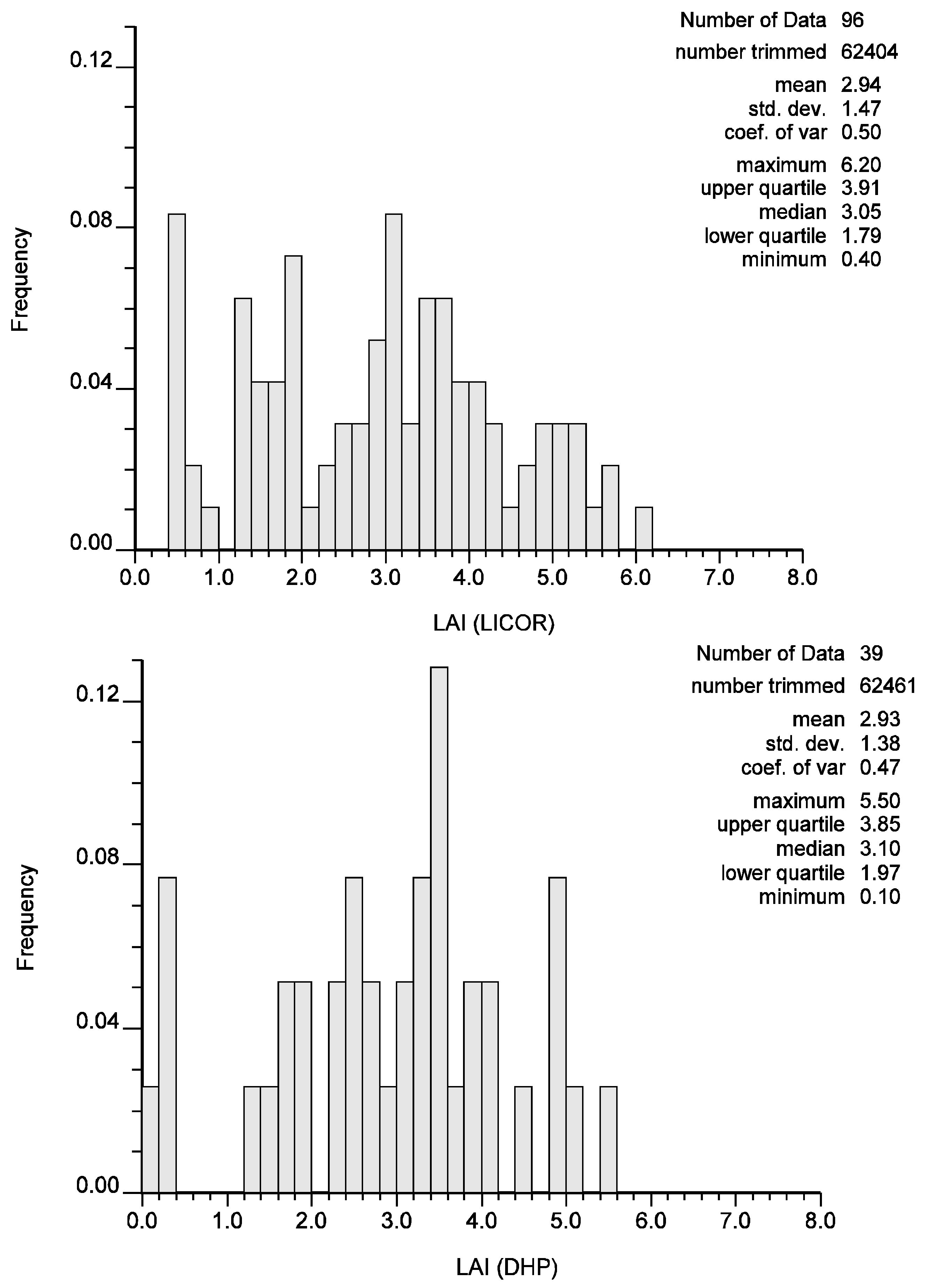
4.1. LAI Field Measurements
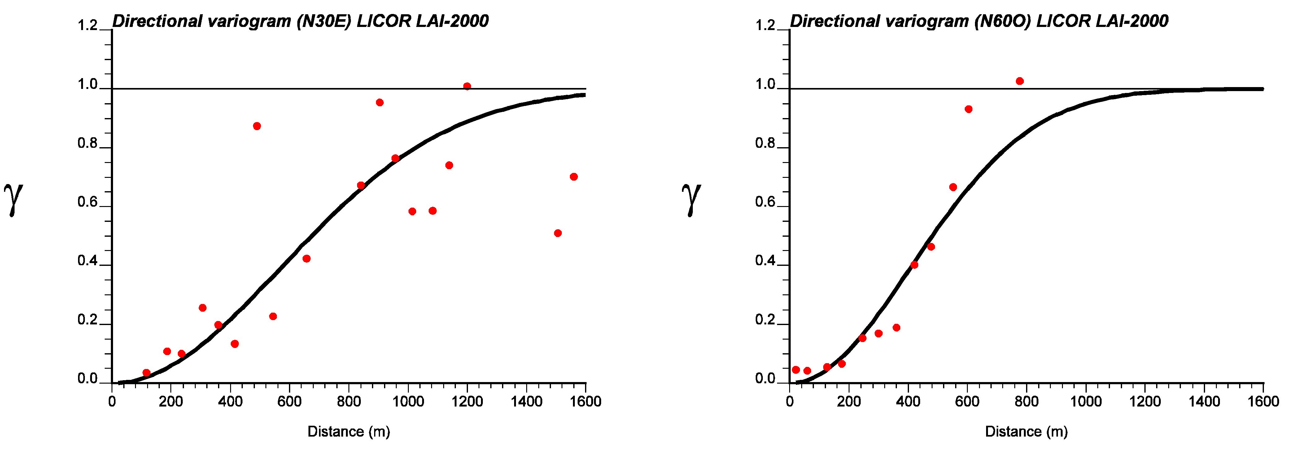
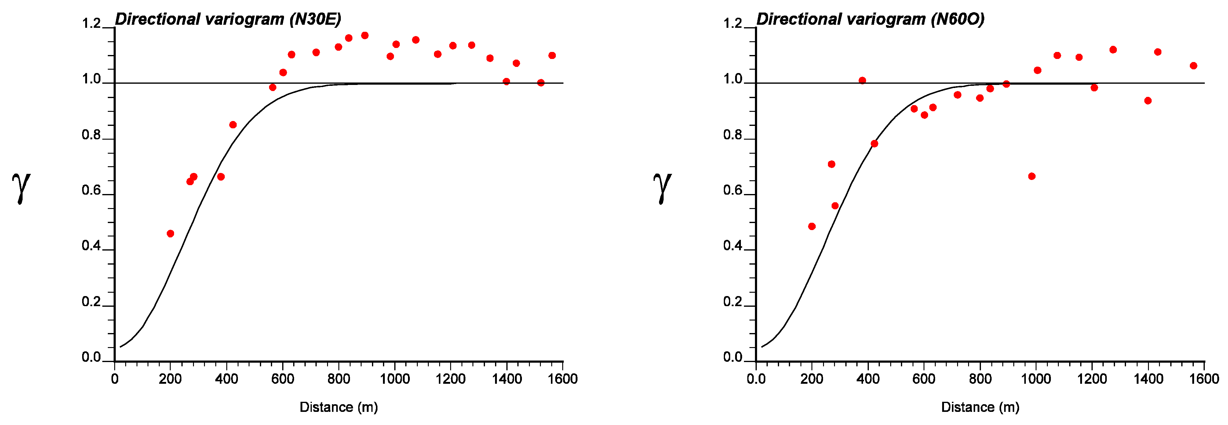
4.2. Modeling Spatial Continuity
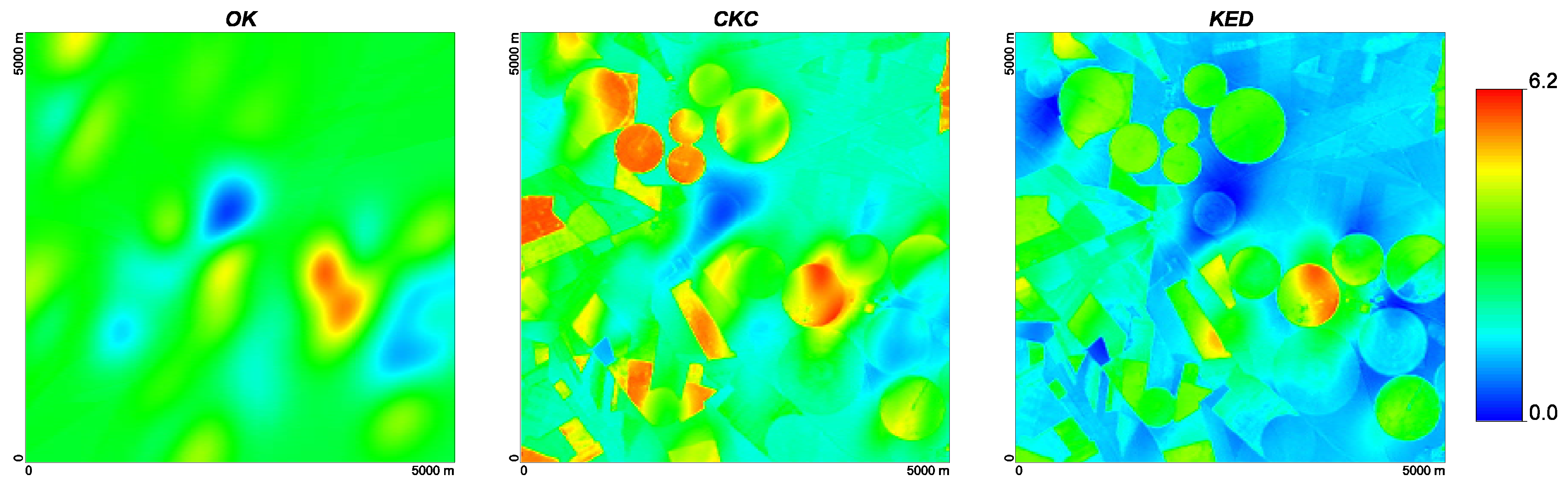
4.3. LAI Predictions

| Model | Slope | Intercept | r | RMSE |
| OK | 0.7 | 0.7 | 0.7 | 1.3 |
| CKC | 0.9 | 0.4 | 0.8 | 1.2 |
| KED | 0.9 | 0.5 | 0.9 | 0.8 |
| Model | Slope | Intercept | r | RMSE |
| OK | 0.10 | 2.8 | 0.3 | 2.4 |
| CKC | 0.6 | 2.1 | 0.8 | 1.9 |
| KED | 0.6 | 1.3 | 0.9 | 1.2 |
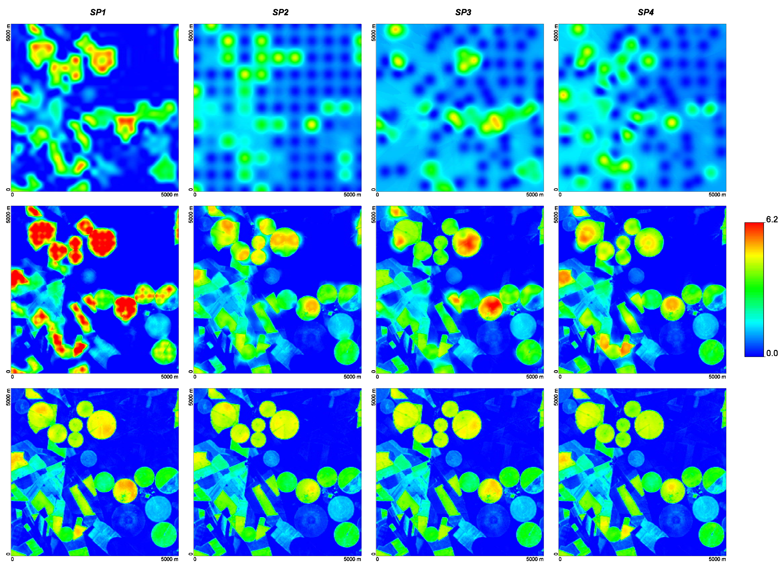
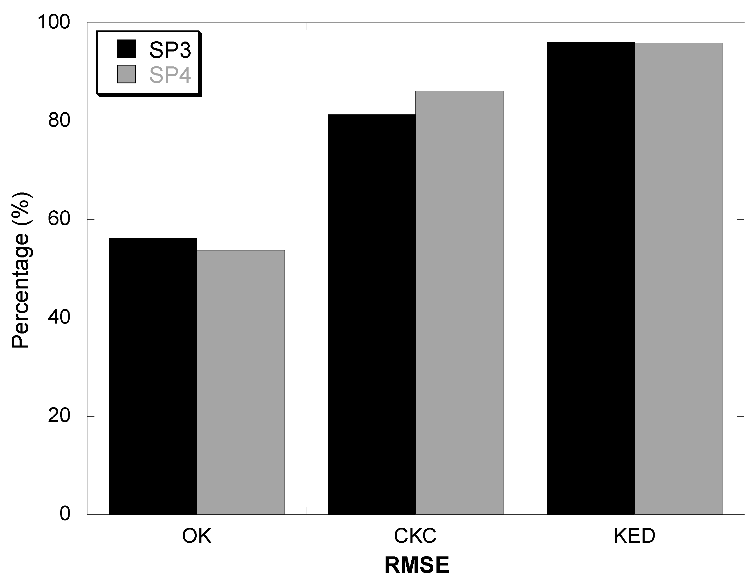
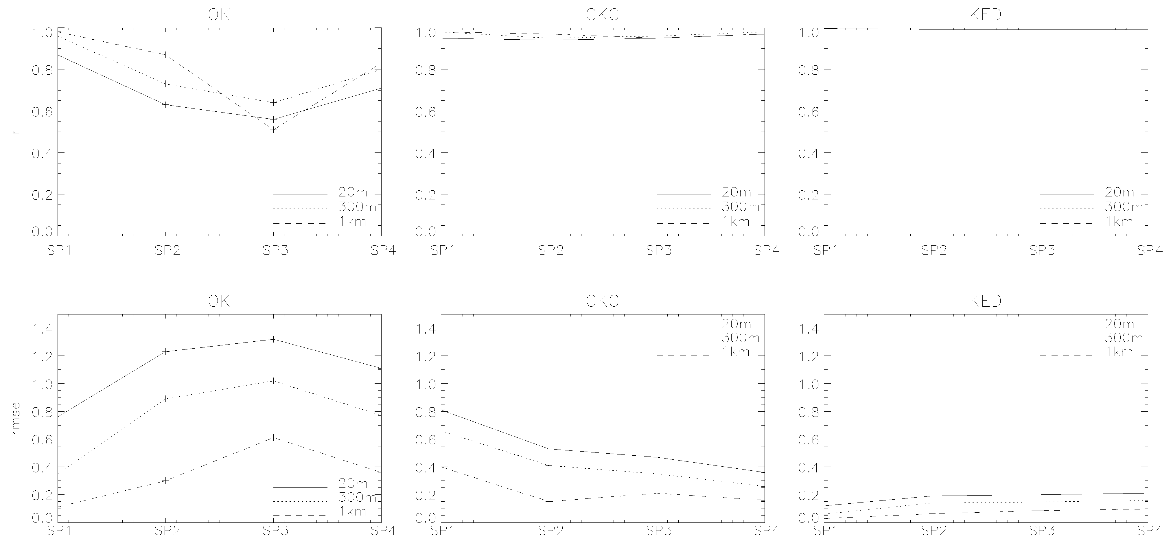
4.4. Efficient Configuration
| Spatial sampling | Type | Regular spacing | Number of samples |
| SP1 | Systematic | 200 m | 676 |
| SP2 | Systematic | 500 m | 121 |
| SP3 | Stratified | - | 61 (veg.)+ 51 (soil) |
| SP4 | Stratified | - | 36 (veg.)+ 51 (soil) |

| Model | Slope | Intercept | r | RMSE |
| OK | ||||
| SP1 | 0.8 | 0.2 | 0.9 | 0.7 |
| SP2 | 0.3 | 0.8 | 0.6 | 1.3 |
| SP3 | 0.3 | 0.8 | 0.6 | 1.3 |
| SP4 | 0.3 | 0.8 | 0.7 | 1.2 |
| CKC | ||||
| SP1 | 1.3 | 0.01 | 0.9 | 0.8 |
| SP2 | 0.9 | 0.18 | 0.9 | 0.5 |
| SP3 | 0.9 | 0.18 | 0.9 | 0.5 |
| SP4 | 0.9 | 0.1 | 0.9 | 0.4 |
| KED | ||||
| SP1 | 0.9 | 0.04 | 0.9 | 0.13 |
| SP2 | 0.9 | 0.07 | 0.9 | 0.2 |
| SP3 | 0.9 | 0.1 | 0.9 | 0.18 |
| SP4 | 0.9 | 0.1 | 0.9 | 0.2 |

4.5. Spatial Resolution Influence
5. Conclusions
Acknowledgments
References and Notes
- Sellers, P.J.; Dickinson, R.E.; Randall, D.A.; Betts, A.K.; Hall, F.G.; Berry, J.A.; Collatz, G.J.; Denning, A.S.; Mooney, H.A.; Nobre, C.A.; Sato, N.; Field, C.B.; Henderson-Sellers, A. Modelling the exchanges of energy, water, and carbon between continents and the atmosphere. Science 1997, 275, 502–509. [Google Scholar] [CrossRef] [PubMed]
- Liu, J.; Chen, J.M.; Cihlar, J.; Park, W.M. A process-based boreal ecosystem productivity simulator using remote sensing inputs. Remote Sens. Environ. 1997, 62, 158–175. [Google Scholar] [CrossRef]
- Bonan, G. Importance of leaf area index and forest type when estimating photosynthesis in boreal forests. Remote Sens. Environ. 1993, 43, 303–314. [Google Scholar] [CrossRef]
- Running, S.W.; Peterson, D.; Spanner, M.; Teuber, K. Remote sensing of coniferous forest leaf area. Ecology 1996, 67, 273–276. [Google Scholar] [CrossRef]
- Turner, D.P.; Cohen, W.B.; Kennedy, R.E.; Fassnacht, K.S.; Briggs, J.M. Relationships between leaf area index, fAPAR, and net primary production of terrestrial ecosystems. Remote Sens. Environ. 1999, 70, 52–68. [Google Scholar] [CrossRef]
- Buermann, W.; Dong, J.; Zeng, X.; Myneni, R.B.; Dickinson, R.E. Evaluation of the utility of satellite-based vegetation leaf area index data for climate simulations. J. Climate 2001, 14, 3536–3550. [Google Scholar] [CrossRef]
- Cohen, W.B.; Maiersperger, T.K.; Gower, S.T.; Turner, D.P. An improved strategy for regression of biophysical variables and Landsat ETM+ data. Remote Sens. Environ. 2003, 84, 561–571. [Google Scholar] [CrossRef]
- Fassnacht, K.S.; Gower, S.T.; Mackenzie, M.D.; Nordhein, E.V.; Lillesand, T.M. Estimating the leaf area index of north central Wisconsin forests using the Landsat Thematic Mapper. Remote Sens. Environ. 1997, 61, 229–245. [Google Scholar] [CrossRef]
- Chen, J.M.; Pavlic, G.; Brown, L.; Cihlar, J.; Leblanc, S.G.; White, H.P.; Hall, R.J.; Peddle, D.R.; King, D.J.; Trofymow, J.A.; Swift, E.; Van der Sanden, J.; Pellikka, P.K.E. Derivation and validation of Canada wide coarse resolution leaf area index maps using high resolution satellite imagery and ground measurements. Remote Sens. Environ. 2002, 80, 165–184. [Google Scholar] [CrossRef]
- Morisette, J.T.; Baret, F.; Privette, J.L.; Myneni, R.B.; Nickeson, J.E.; Garrigues, S.; Shabanov, N.V.; Weiss, M.; Fernandes, R.A.; Leblanc, S.G.; Kalacska, M.; Sánchez-Azofeifa, G.; Chubey, M.; Rivard, B.; Stenberg, P.; Rautiainen, M.; Voipio, P.; Manninen, T.; Pilant, A.N.; Lewis, T.E.; Iiames, J.S.; Colombo, R.; Meroni, M.; Busetto, L.; Cohen, W.B.; Turner, D.P.; Warner, E.D.; Petersen, G.W.; Seufert, G.; Cook, R. Validation of global moderate resolution LAI products: A framework proposed within the CEOS land product validation subgroup. IEEE Trans. Geosci. Remote Sens. 2006, 44, 1804–1817. [Google Scholar]
- Martínez, B.; García-Haro, F. J.; Camacho-de Coca, F. Derivation of high-resolution leaf area index maps in support of validation activities. Application to the cropland Barrax site. Agr. Forest Meteorol. 2009, 149, 130–145. [Google Scholar] [CrossRef]
- Steel, R.; Torrie, J. Principles and Procedures of Statistics: A Biometrical Approach, 2nd ed.; McGraw-Hill: New York, NY, USA, 1980. [Google Scholar]
- Chen, J.; Cihlar, J. Retrieving LAI of boreal conifer forests using Landsat TM images. Remote Sens. Environ. 1996, 55, 153–162. [Google Scholar] [CrossRef]
- White, J.; Running, S.; Nemani, R.; Keane, R.; Ryan, K. Measurement and remote sensing of LAI in rocky mountain montane ecosystems. Canad. J. Forest Res. 1997, 27, 1714–1727. [Google Scholar] [CrossRef]
- Curran, P.J.; Hay, A.M. The importance of measurement error for certain procedure in remote sensing of optical wavelengths. Photogramm. Eng. Remote Sensing 1986, 52, 229–241. [Google Scholar]
- Weiss, M. Valeri 2003: Barrax Site (Cropland); Ground data processing & Production of the level 1 high resolution maps; INRA-CSE: Avignon, France, July 2003; Available online: http://www.avignon.inra.fr/valeri (accessed on 19 November 2010).
- Tabachnick, B.; Fidell, L. Using Multivariate Statistics, 2nd ed.; Harper Collins Publishers: London, UK, 1989. [Google Scholar]
- Lee, K.; Cohen, W.; Kennedy, R.E.; Maiersperger, T.K.; Gower, S.T. Hyperspectral versus multispectral data for estimating leaf area index in four different biomes. Remote Sens. Environ. 2004, 91, 508–520. [Google Scholar] [CrossRef]
- Fernandes, R.T.; Leblanc, S.G. Parametric (modified least squares) and non-parametric (Theil–Sen) linear regressions for predicting biophysical parameters in the presence of measurement errors. Remote Sens. Environ. 2005, 95, 303–316. [Google Scholar] [CrossRef]
- Berterretche, M.; Hudak, A.T.; Cohen, T.W.; Maiersperger, T.K.; Gower, S.T.; Dungan, J. Comparison of regression and geostatistical methods for mapping Leaf Area Index (LAI) with Landsat ETM+ data over a boreal forest. Remote Sens. Environ. 2005, 96, 49–61. [Google Scholar] [CrossRef]
- Hudak, A.T.; Lefsky, M.A.; Cohen, W.B.; Berterretche, M. Integration of lidar and Landsat ETM+ data for estimating and mapping forest canopy height. Remote Sens. Environ. 2002, 82, 397–416. [Google Scholar] [CrossRef]
- Bourennane, H.; King, D.; Couturier, A. Comparison of kriging with external drift and simple linear regression for prediction soil horizon thickness with different sample densities. Geoderma 2000, 97, 255–271. [Google Scholar] [CrossRef]
- Goovaerts, P. Geostatistical approaches for incorporating elevation into the spatial interpolation of rainfall. J. Hydrol. 2000, 228, 113–129. [Google Scholar] [CrossRef]
- Triantafilis, J.; Odeh, I.O.A.; McBratney, A.B. Five geostatistical models to predict soil salinity from electromagnetic induction data across irrigated cotton. Soil Sci. Soc. Amer. J. 2001, 65, 869–878. [Google Scholar] [CrossRef]
- Bekele, A.; Downer, R.G.; Wolcott, M.C.; Hudnall, W.H.; Moore, S.H. Comparative evaluation of spatial prediction methods in a field experiment for mapping soil potassium. Soil Sci. 2003, 168, 15–28. [Google Scholar] [CrossRef]
- Dobermann, A.; Ping, J.L. Geostatistical integration of yield monitor data and remote sensing improves yield maps. Agron. J. 2004, 96, 285–297. [Google Scholar] [CrossRef]
- Matheron, G. Principles of geostatistics. Economic Geol. 1963, 58, 1246–1266. [Google Scholar] [CrossRef]
- Burgess, T.M.; Webster, R. Optimal interpolation and isarithmic mapping of soil properties. The semi-variogram and punctual Kriging. J. Soil Sci. 1980, 31, 315–331. [Google Scholar] [CrossRef]
- Lakhankar, T.; Jones, A.S.; Combs, C.L.; Sengupta, M.; Vonder Haar, T.H.; Khanbilvardi, R. Analysis of large scale spatial variability of soil moisture using a geostatistical method. Sensors 2010, 10, 913–932. [Google Scholar] [CrossRef] [PubMed]
- Kitanidis, P.K.; Vomvoris, E.G. A geostatistical approach to the inverse problem in groundwater modeling (steady state) and one dimensional simulations. Water Resour. Res. 1983, 19, 677–690. [Google Scholar] [CrossRef]
- Yates, S.R.; Warrick, A.W. Estimating soil water content using cokriging. Soil Sci. Soc. Amer. J. 1987, 51, 23–30. [Google Scholar] [CrossRef]
- Li, B.; Yeh, J. Cokriging estimation of the conductivity field under variably saturated flow conditions. Water Resour. Res. 1999, 35, 3663–3674. [Google Scholar] [CrossRef]
- Bruin, S. Predicting the areal extent of land-cover types using classified imagery and Geostatistics. Remote Sens. Environ. 2000, 74, 387–396. [Google Scholar] [CrossRef]
- Burrows, S.N.; Gower, S.T.; Clayton, M.K.; Mackay, D.S.; Ahl, D.E.; Norman, J.M.; Diak, G. Application of Geostatistics to characterize Leaf Area Index (LAI) from flux tower to landscape scales using a cyclic sampling design. Ecosystems 2002, 5, 667–679. [Google Scholar]
- Dungan, J. Spatial prediction of vegetation quantities using ground and image data. Int. J. Remote Sens. 1998, 19, 267–285. [Google Scholar] [CrossRef]
- Isaaks, E.H.; Srivastava, R.M. Applied Geostatistics; Oxford University Press: Oxford, UK, 1989. [Google Scholar]
- Woodcock, C.E.; Strahler, A.H.; Jupp, D.L.B. The use of variograms in remote sensing: I. Scenes Models and Simulated Images. Remote Sens. Environ. 1988, 25, 323–348. [Google Scholar] [CrossRef]
- Xu, W.; Tran, T.; Srivastava, R.M.; Journel, A.G. Integrating seismic data in reservoir modeling: The collocated cokriging alternative. In Proceedings of 67th Annual Technical Conference and Exhibition of the Society of Petroleum Engineers, Washington, DC, USA, October 4–7, 1992; SPE paper # 24742. pp. 833–842.
- Kuzyakova, I.F.; Romanenkov, V.A.; Kuzyakov, Y.V. Geostatistics in soil agrochemical studies. Eurasian Soil Sci. 2001, 34, 1011–1017. [Google Scholar]
- Deutsch, C.; Journel, A. GSLIB, Geostatistical Software Library and User’s Guide, 2nd ed.; Oxford University Press: New York, NY, USA, 1998. [Google Scholar]
- Goovaerts, P. Geostatistics for Natural Resources Evaluation; Oxford University Press: New York, NY, USAZ, 1997. [Google Scholar]
- Bolle, H.J.; DeBruin, H.A.R.; Stricker, H. EFEDA: European field experiment in a desertification threatened area. Annales Geophysique 1993, 11, 173–189. [Google Scholar]
- Moreno, J.; Alonso, L.; Gonzalez, M.C.; Garcia, J.C.; Cunat, C.; Montero, F.; Brasa, A.; Botella, O.; Zomer, R.J.; Ustin, S.L. Vegetation properties from imaging data acquired at Barrax in 1998, 1999 and 2000. In Proceedings of DAISEX Final Results Workshop, Noordwijk, The Netherlands, March 15–16, 2001; ESA SP-499. pp. 197–207.
- Martínez, B.; Camacho-de Coca, F.; García-Haro, F.J. Estimación de parámetros biofísicos de vegetación utilizando el método de la cámara hemisférica. Revista de Teledetección 2006, 26, 5–17. [Google Scholar]
- LI-COR. LAI-2000 Plant Canopy Analyser. Instruction Manual; LICOR: Lincoln, NE, USA, 1992. [Google Scholar]
- Ross, J. The Radiation Regime and Architecture of Plant Stands; Dr W. Junk Publishers: The Hague, The Netherlands, 1981. [Google Scholar]
- Welles, J.M. Some indirect methods of estimating canopy structure. Remote Sens. Rev. 1990, 5, 31–43. [Google Scholar] [CrossRef]
- Welles, J.M.; Norman, J.M. Instrument for indirect measurement of canopy architecture. Agron. J. 1991, 83, 818–825. [Google Scholar] [CrossRef]
- Bonhomme, R.; Varlet Granger, C.; Chartier, P. The use of photographs for determining the leaf area index of young crops. Photosynthesis 1972, 8, 299–301. [Google Scholar]
- Rich, P.M. Characterizing plant canopies with hemispherical photographs. Remote Sens. Rev. 1990, 5, 13–29. [Google Scholar] [CrossRef]
- Jonckheere, I.; Fleck, S.; Nackaerts, K.; Muys, B.; Coppin, P.; Weiss, M.; Baret, F. Methods for leaf area index determination. Part I: Theories, techniques and instruments. Agr. Forest Meteorol. 2004, 121, 19–35. [Google Scholar] [CrossRef]
- Rich, P.M.; Clark, D.B.; Clark, D.A.; Oberbauer, S.F. Long-term study of solar radiation regimes in a tropical wet forest using quantum sensors and hemispherical photography. Agr. Forest Meteorol. 1993, 65, 107–127. [Google Scholar] [CrossRef]
- Martínez, B. Caracterización espacial de parámetros biofísicos de la cubierta vegetal para la validación de productos derivados mediante teledetección. Aplicación de técnicas geoestadísticas. Ph.D. Thesis, University of Valencia, Valencia, Spain, 2006; p. 242. [Google Scholar]
- Tucker, C. Red and infrared linear combinations for monitoring vegetation. Remote Sens. Environ. 1979, 8, 127–150. [Google Scholar] [CrossRef]
- Geerken, R.; Ilaiwi, M. Assessment of rangeland degradation and development of a strategy for rehabilitation. Remote Sens. Environ. 2004, 90, 490–504. [Google Scholar] [CrossRef]
- Justice, C.O.; Townshend, J.R.G.; Holben, B.N.; Tucker, C.J. Analysis of the phenology of global vegetation using meteorological satellite data. Int. J. Remote Sens. 1985, 6, 1271–1318. [Google Scholar] [CrossRef]
- Huete, A.R. Spectral response of a plant canopy with different soil backgrounds. Remote Sens. Environ. 1985, 17, 37–53. [Google Scholar] [CrossRef]
- Bogaert, P.; Russo, D. Optimal spatial sampling design for the estimation of the variogram based on a least squares approach. Water Resour. Res. 1999, 35, 1275–1289. [Google Scholar] [CrossRef]
- Müller, W.G.; Zimmerman, D.L. Optimal designs for variogram estimation. Environmetrics 1999, 10, 23–37. [Google Scholar] [CrossRef]
- Liang, S. Quantitative Remote Sensing of Land Surfaces; John Wiley & Sons, Inc.: New York, NY, USA, 2004. [Google Scholar]
- Almeida, A.S.; Journel, A.G. Joint simulation of multiple variables with a Markov-type coregionalization model. Math. Geol. 1994, 26, 565–588. [Google Scholar] [CrossRef]
- Tian, Y.; Woodcock, C.E.; Wang, Y.; Privette, J.L.; Shabanov, N.V.; Zhou, L.; Zhang, Y.; Buermann, W.; Dong, J.; Veikkanen, B.; Häme, T.; Andersson, K.; Ozdogan, M.; Knyazikhin, Y.; Myneni, R.B. Multiscale analysis and validation of MODIS LAI product over Maun, Botswana. I: Uncertainty assessment. Remote Sens. Environ. 2002, 83, 414–430. [Google Scholar] [CrossRef]
© 2010 by the authors; licensee MDPI, Basel, Switzerland. This article is an open access article distributed under the terms and conditions of the Creative Commons Attribution license (http://creativecommons.org/licenses/by/3.0/).
Share and Cite
Martinez, B.; Cassiraga, E.; Camacho, F.; Garcia-Haro, J. Geostatistics for Mapping Leaf Area Index over a Cropland Landscape: Efficiency Sampling Assessment. Remote Sens. 2010, 2, 2584-2606. https://doi.org/10.3390/rs2112584
Martinez B, Cassiraga E, Camacho F, Garcia-Haro J. Geostatistics for Mapping Leaf Area Index over a Cropland Landscape: Efficiency Sampling Assessment. Remote Sensing. 2010; 2(11):2584-2606. https://doi.org/10.3390/rs2112584
Chicago/Turabian StyleMartinez, Beatriz, Eduardo Cassiraga, Fernando Camacho, and Javier Garcia-Haro. 2010. "Geostatistics for Mapping Leaf Area Index over a Cropland Landscape: Efficiency Sampling Assessment" Remote Sensing 2, no. 11: 2584-2606. https://doi.org/10.3390/rs2112584
APA StyleMartinez, B., Cassiraga, E., Camacho, F., & Garcia-Haro, J. (2010). Geostatistics for Mapping Leaf Area Index over a Cropland Landscape: Efficiency Sampling Assessment. Remote Sensing, 2(11), 2584-2606. https://doi.org/10.3390/rs2112584