Polarized Bidirectional Reflectance Distribution Function Matrix Derived from Two-Scale Roughness Theory and Its Applications in Active Remote Sensing

Abstract

A polarized bidirectional reflectance distribution function (pBRDF) matrix was developed based on the two-scale roughness theory to provide consistent simulations of fully polarized microwave emission and scattering, required for the ocean–atmosphere-coupled radiative transfer model. In this study, the potential of the two-scale pBRDF matrix was explored for simulating ocean full-polarization backscattering and bistatic-scattering normalized radar cross sections (NRCSs). Comprehensive numerical simulations of the two-scale pBRDF matrix across the L-, C-, X-, and Ku-bands were carried out, and the simulations were compared with experimental data, classical electromagnetic, and GMFs. The results show that the two-scale pBRDF matrix demonstrates reasonable dependencies on ocean surface wind speeds, relative wind direction (RWD), geometries, and frequencies and has a reliable accuracy in general. In addition, the two-scale pBRDF matrix simulations were compared with the observations from the advanced scatterometer (ASCAT) onboard MetOP-C satellites, with a correlation coefficient of 0.9634 and a root mean square error (RMSE) of 2.5083 dB. In the bistatic case, the two-scale pBRDF matrix simulations were compared with Cyclone Global Navigation Satellite System (CYGNSS) observations, demonstrating a good correlation coefficient of 0.8480 and an RMSE of 1.2859 dB. In both cases, the two-scale pBRDF matrix produced fairly good simulations at medium-to-high wind speeds. The relatively large differences at low wind speeds (<5 m/s) were due probably to the swell effects. This study proves that the two-scale pBRDF matrix is suitable for the applications of multiple types of active instruments and can consistently simulate the ocean surface passive and active signals.

1. Introduction

Spaceborne microwave instruments are crucial for the remote sensing of ocean surface parameters. Passive instruments including WindSat, TMI, SSM/I, and AMSR2 have been used for retrieving sea surface temperature (SST), sea surface salinity (SSS), wind speed, and sea ice concentration [1,2,3,4,5]. Active instruments such as ASCAT, FY-3E WindRAD, and JASON are used for measuring ocean surface wind vectors and wave heights [6,7,8]. The passive and active microwave signals from the ocean surface are interrelated. In polarized radiative transfer theory, ocean surface passive signals are contributed from the emissivity vector and reflectivity vector. According to polarized Kirchhoff’s law, the emissivity vector and reflectivity vector should be complementary to unity [9,10,11]. The reflectivity vector is the integral of the ocean surface bidirectional reflectance over the upper hemisphere, while the bidirectional reflectance, including bistatic scattering and backscattering, which are commonly used by active instruments, can be obtained using the pBRDF matrix [12,13,14]. Thus, the ocean surface-polarized microwave emission and scattering signals can be consistently simulated based on the pBRDF matrix for the combined active–passive applications. To the best of our knowledge, there have been no studies addressing the simultaneous modeling of fully polarized active and passive signals utilizing the pBRDF matrix.

An electromagnetic model has been developed at the Universite’ Catholique de Louvain (UCL) for the simulation of microwave measurements in spaceborne passive radiometers, active scatterometers, and altimeters [15,16]. This model, hereafter called the UCL model, utilizes bistatic-scattering coefficients to compute backscattering coefficients and emissivity based on the two-scale roughness theory. However, the model does not consider the second-order terms for the small perturbation method (SPM) and, thus, is inaccurate in simulating the depolarization effect. Also, the UCL model does not have full polarization simulation capability. Recently, a Passive and Active Reference Microwave to Infrared Ocean (PARMIO) model was been developed to support passive and active applications [17]. Both the UCL and PARMIO models simulate the backscattering NRCS and emissivity, but they do not support the simulation of circularly polarized bistatic-scattering NRCS, which is required for Global Navigation Satellite Systems’ reflectometry (GNSS-R). A generic fully polarimetric reflectivity matrix is developed based on the two-scale roughness theory for simulations of emissivity vectors in passive remote sensing [18]. This reflectivity matrix is essentially a two-scale pBRDF matrix that encompasses scattering contributions from ocean surface large-scale roughness, first-order and second-order SPM of small-scale roughness, as well as sea foam. The study demonstrated that this two-scale pBRDF matrix can reasonably reproduce the ocean surface bidirectional reflectance and more accurately simulate the emissivity vector compared with the geometrical optic (GO) pBRDF matrix. Considering the relationship between the NRCS and the BRDF [19], the two-scale pBRDF matrix may be well used in simulating ocean surface active signals.

In this study, we expanded the utilization of the two-scale pBRDF matrix to microwave active remote sensing for simulating fully polarimetric backscattering and bistatic-scattering NRCS to explore its potential in providing a consistent emission and scattering simulation for joint applications of microwave passive and active instruments. The remainder of this paper is organized as follows: Section 2 provides a brief description of the two-scale pBRDF matrix and demonstrates the derivations of linearly and circularly polarized NRCSs from two-scale pBRDF matrix elements. In Section 3, numerical simulations are presented, showcasing fully polarimetric backscattering and bistatic-scattering NRCSs for various geometries and wind conditions. Also, the comparisons between microwave active observations and the two-scale pBRDF matrix simulations are shown. The discussion and conclusions are presented in Section 4 and Section 5, respectively.

2. Model and Method

2.1. Two-Scale pBRDF Matrix

Scattering calculations are conducted in two major types of coordinate systems: the forward-scattering alignment (FSA) convention and the backscatter alignment (BSA) convention. The two-scale pBRDF matrix is developed based on the FSA convention. In the FSA convention, the backscattering direction corresponds to ${\theta }^s={\theta }^i,{\phi }^s={\phi }^i+\pi$, while the specular direction corresponds to ${\theta }^s={\theta }^i,{\phi }^s={\phi }^i$, which is a special case for forward scattering [20]. Figure 1 illustrates the geometrical configurations for wave scattering from the ocean surface in the FSA convention, where radiance from the solid angle $d{\mathrm{\Omega }}^i$ and centered on the zenith angle ${\theta }^i$ and azimuth angle ${\phi }^i$ is incident on an ocean surface microfacet $dA$ (pink area). Radiance is scattered from the ocean surface and observed within the solid angle $d{\mathrm{\Omega }}^s$ at the zenith angle ${\theta }^s$ and azimuth angle ${\phi }^s$. Three typical scattering geometries are depicted, including backscattering, forward scattering, and out-of-plane scattering. The positive x-axis of the coordinate system points in the direction of the wind flow. Therefore, the scattering azimuth angle is equal to the RWD.

The two-scale roughness theory has demonstrated good performances in simulating surface scattering and emission from ocean surfaces [21,22,23,24,25,26]. The two-scale roughness theory simulates the ocean surface as large-scale gravity waves and small-scale capillary waves, with the small-scale waves riding on top of the large-scale waves. Based on the two-scale roughness theory, a general fully polarimetric two-scale reflectivity matrix (TSRM) has been developed [18]. The TSRM incorporates the large-scale scattering of the ocean surface using the GO approach and accounts for small-scale scattering using the SPM up to the second order. Essentially, the TSRM is a two-scale pBRDF matrix.

The pBRDF matrix is defined as the ratio of the scattered radiance vector to the incident irradiance vector and can be expressed as follows:

$$R({\theta }^i,{\phi }^i;{\theta }^s,{\phi }^s)=\frac{d{I}^s({\theta }^s,{\phi }^s)}{d{E}^i({\theta }^i,{\phi }^i)}=\frac{d{I}^s({\theta }^s,{\phi }^s)}{I_i({\theta }^i,{\phi }^i)\cos {\theta }^{i}d{\mathrm{\Omega }}^i}$$

(1)

where $d{I}^s$ represents the scattered radiance vector, and $d{E}^i$ denotes the incident irradiance vector. The incident irradiance vector is equivalent to the product of the incident radiance vector and the projected solid angle $\cos {\theta }^{i}d{\mathrm{\Omega }}^i$ [27,28,29,30]. The relationship between the reflectivity matrix TSRM $A$ and the two-scale pBRDF matrix $R$ is given as follows [31,32]:

$$A({\theta }^i,{\phi }^i;{\theta }^s,{\phi }^s)=R({\theta }^i,{\phi }^i;{\theta }^s,{\phi }^s)\times \cos {\theta }^i$$

(2)

Referring to the TSRM expression provided by [18] and Equation (2), the two-scale pBRDF matrix can be defined as follows:

$$\begin{array}{c}R({\theta }^i,{\phi }^i;{\theta }^s,{\phi }^s)=A({\theta }^i,{\phi }^i;{\theta }^s,{\phi }^s)/\cos ({\theta }^i)\hfill \\ \begin{array}{cc}=\frac{1}{\cos ({\theta }^i)}\times \left(\begin{array}{cccc}{A}_{vvvv}& A_{vhvh}& \mathrm{Re}(A_{vhvv})& \mathrm{Im}(A_{vhvv})\\ A_{hvhv}& A_{hhhh}& \mathrm{Re}(A_{hhhv})& \mathrm{Im}(A_{hhhv})\\ 2\mathrm{Re}(A_{vvhv})& 2\mathrm{Re}(A_{vhhh})& \mathrm{Re}(A_{vvhh}+A_{vhhv})& \mathrm{Im}(A_{hhvv}+A_{hvvh})\\ 2\mathrm{Im}(A_{vvhv})& 2\mathrm{Im}(A_{vhhh})& \mathrm{Im}(A_{vvhh}+A_{vhhv})& \mathrm{Re}(A_{hhvv}-A_{hvvh})\end{array}\right)& \end{array}\hfill \\ =\left(\begin{array}{cccc}{R}_{vvvv}& R_{vhvh}& \mathrm{Re}(R_{vhvv})& \mathrm{Im}(R_{vhvv})\\ R_{hvhv}& R_{hhhh}& \mathrm{Re}(R_{hhhv})& \mathrm{Im}(R_{hhhv})\\ 2\mathrm{Re}(R_{vvhv})& 2\mathrm{Re}(R_{vhhh})& \mathrm{Re}(R_{vvhh}+R_{vhhv})& \mathrm{Im}(R_{hhvv}+R_{hvvh})\\ 2\mathrm{Im}(R_{vvhv})& 2\mathrm{Im}(R_{vhhh})& \mathrm{Im}(R_{vvhh}+R_{vhhv})& \mathrm{Re}(R_{hhvv}-R_{hvvh})\end{array}\right)\hfill \end{array}$$

(3)

Figure 2 depicts the spatial distribution of the two-scale pBRDF matrix at 37 GHz in the upper hemisphere in the specular direction. All the subplots are presented in polar coordinates, with the radial axis representing variations in the zenith angle and the tangential axis representing variations in the azimuth angle, with 0°, 90°, and 180°, respectively, representing upwind, crosswind, and downwind directions. Figure 2 shows that each element is symmetric with respect to the wind direction, and the evenly/oddly symmetric elements have cosine/sine azimuth harmonic components, with the extremes falling in the correct azimuth angles. These characterizations demonstrate that the two-scale pBRDF matrix can reasonably reproduce the bidirectional reflectance of the ocean surface in the specular direction. Figure 3 illustrates the emissivity vector derived from the two-scale pBRDF matrix and the comparisons with other emissivity models, namely, FASTEM 6 and SURFEM, which are fast emissivity models developed by the European Center for Medium-range Weather Forecasts in 2015 and 2023, respectively [33,34]. The accuracies of FASTEM 6 for the vertical and horizontal components have been widely proven through satellite measurements, but the third and fourth components, which come from FASTEM 3, have been proven to be unreliable [34,35]. The vertical and horizontal components of emissivity calculated by the two-scale pBRDF matrix are comparable to FASTEM 6, and the maximum differences, respectively, are 0.002 and 0.004. The third and fourth components are comparable to SURFEM. The comparisons highlight that the two-scale pBRDF matrix is a viable tool for reasonably calculating emissivity.

2.2. Relationship between NRCSs and the Two-Scale pBRDF Matrix

The quantity of active measurement is NRCS. The bistatic linear NRCS can be defined as follows [19]:

$${\sigma }_{\alpha \beta {\alpha }^{\prime }{\beta }^{\prime }}^0({\theta }^i,{\phi }^i;{\theta }^s,{\phi }^s)=\underset{R\to \infty }{\lim }4\pi R^2\frac{〈E_{\alpha \beta }({\theta }^s,{\phi }^s)E_{\alpha \beta }^{*}({\theta }^s,{\phi }^s)〉}{A{E}_{{\alpha }^{\prime }{\beta }^{\prime }}^2({\theta }^i,{\phi }^i)}$$

(4)

where $E_{\alpha \beta }({\theta }^s,{\phi }^s)$ represents the scattering field for the polarization state $\alpha \beta$; $E_{{\alpha }^{\prime }{\beta }^{\prime }}({\theta }^i,{\phi }^i)$ denotes the incident field for the polarization state ${\alpha }^{\prime }{\beta }^{\prime }$; $A$ represents the irradiation area; 〈 〉 represents the statistical average of the scattering intensity of the rough surface; $R$ represents the distance between the scattering field and the incident field; and ${\sigma }_{\alpha \beta {\alpha }^{\prime }{\beta }^{\prime }}^0$ ($\alpha ,\beta ,{\alpha }^{\prime },{\beta }^{\prime }=v,h$) represents the bistatic NRCS.

When the receiving aperture is $A_r$, the ratio of scattering power received $\Delta P_s$ and incident power $P_i$ can be expressed as follows:

$$\frac{\Delta P_s}{P_i}=\frac{A_r〈E_{\alpha \beta }({\theta }^s,{\phi }^s)E_{\alpha \beta }^{*}({\theta }^s,{\phi }^s)〉}{A{E}_{{\alpha }^{\prime }{\beta }^{\prime }}^2({\theta }^i,{\phi }^i)}$$

(5)

According to Equations (4) and (5), the following equation can be derived:

$${\sigma }_{\alpha \beta {\alpha }^{\prime }{\beta }^{\prime }}^0=4\pi \cos {\theta }^i\frac{d{P}_s}{P_{i}d\mathrm{\Omega }}$$

(6)

where $d\mathrm{\Omega }=\underset{R\to \infty }{\lim }{A}_r/R^2$.

Equation (1) defines the pBRDF matrix. For simplicity, here we have omitted the symbols denoting the polarizations. $d{E}^i$ is expressed as the radiant flux $f_i$ per unit area

$$d{E}^i=\frac{d{f}_i}{dA}$$

(7)

where $d{I}^s$ is the scattered radiance and represents the radiant flux per unit area and solid angle, which can be expressed as follows:

$$d{I}^s=\frac{d^2{f}_s}{d\mathrm{\Omega }dA\cos {\theta }^s}$$

(8)

From Equations (1), (7), and (8), the pBRDF matrix of the rough surface can be obtained as follows:

$$R({\theta }^i,{\phi }^i;{\theta }^s,{\phi }^s)=\frac{d^2{f}_s}{d\mathrm{\Omega }dA\cos {\theta }^s}/\frac{d{f}_i}{dA}$$

(9)

For an expanded uniform surface element, $d{f}_i/dA$ and $d{f}_s/dA$ can be the incident power $P_i$ and scattered power $P_s$ irradiating the unit area, respectively. Therefore, the above equation can be rewritten as follows:

$$R({\theta }^i,{\phi }^i;{\theta }^s,{\phi }^s)=\frac{d{P}_s}{P_{i}d\mathrm{\Omega }\cos {\theta }^s}$$

(10)

Substituting Equation (10) into Equation (6), the relationship between the pBRDF matrix and the linear bistatic NRCS can be obtained as follows:

$${\sigma }_{\alpha \beta {\alpha }^{\prime }{\beta }^{\prime }}^0({\theta }^i,{\phi }^i;{\theta }^s,{\phi }^s)=4\pi \cos {\theta }^i\cos {\theta }^s\times R_{\alpha \beta {\alpha }^{\prime }{\beta }^{\prime }}({\theta }^i,{\phi }^i;{\theta }^s,{\phi }^s)$$

(11)

In active remote sensing, the polarization states where $\alpha ={\alpha }^{\prime },\beta ={\beta }^{\prime }$ are those of most interest. These polarizations correspond to $vv$, $hh$, $vh$, and $hv$. By utilizing Equations (3) and (11), these polarizations can be expressed using corresponding elements of the two-scale pBRDF matrix as follows:

$$\left(\begin{array}{cc}{\sigma }_{vv}^0& {\sigma }_{vh}^0\\ {\sigma }_{hv}^0& {\sigma }_{hh}^0\end{array}\right)=4\pi \cos {\theta }^i\cos {\theta }^s\left(\begin{array}{cc}{R}_{vvvv}& R_{vhvh}\\ R_{hvhv}& R_{hhhh}\end{array}\right)$$

(12)

Equation (12) is suitable for calculating linear NRCSs at various combinations of incident and scattering configurations. The circularly polarized NRCS can be achieved by appropriately transforming the polarization basis once a fully polarimetric characterization in the linear basis is available [36]

The relationships between scattering coefficients written in a linear and a circular polarization basis are as follows [37]:

$$S_{RR}=(S_{vv}+S_{hh}-i{S}_{vh}+i{S}_{hv})/2$$

(13)

$$S_{RL}=(S_{vv}-S_{hh}+i{S}_{vh}+i{S}_{hv})/2$$

(14)

where $S_{\alpha \beta }(\alpha ,\beta =v,h)$ is the scattering coefficient in a linear polarization basis, and $S_{\alpha \beta }(\alpha ,\beta =R,L)$ is the scattering coefficient in a circular polarization basis.

A detailed derivation from the amplitude scattering coefficient $S_{\alpha \beta }(\alpha ,\beta =v,h)$ to the two-scale pBRDF matrix has been provided in the literature [18]. Then, we can establish the relationships between the circularly polarized NRCSs and the two-scale pBRDF matrix elements through the amplitude scattering coefficient $S_{\alpha \beta }(\alpha ,\beta =v,h)$ as follows:

$${\sigma }_{RL}^0={\sigma }_{LR}^0=\pi \cos {\theta }^s\cos {\theta }^i(R_{vvvv}+R_{hhhh}+R_{vhvh}+R_{hvhv}-2\mathrm{Re}(R_{hhvv}-R_{hvvh}))$$

(15)

$${\sigma }_{RR}^0={\sigma }_{LL}^0=\pi \cos {\theta }^s\cos {\theta }^i(R_{vvvv}+R_{hhhh}-R_{vhvh}-R_{hvhv}+2\mathrm{Re}(R_{vvhh}+R_{vhhv}))$$

(16)

where indices $R$ and $L$ stand for right-handed and left-handed circular polarizations, respectively. GNSS reflectometry commonly uses a right-hand circularly polarized (RHCP) transmitted signal and a left-hand circularly polarized (LHCP) received signal, denoted by ${\sigma }_{LR}^0$.

3. Results

The ocean surface electromagnetic scattering model needs to be able to effectively describe the parameter dependencies of the scattered energy. This section analyzes the dependencies of backscattering and bistatic-scattering NRCSs simulated by the two-scale pBRDF matrix on wind speed, RWD, and geometry, and validates the reasonableness of the dependencies by comparing with simulations of GMFs and physical models or experimental data. The inputs for the two-scale pBRDF matrix include SST, SSS, wind speed, wind direction, incidence zenith angle, incidence azimuth angle, scattering zenith angle, and scattering azimuth angle.

The two-scale pBRDF matrix simulations require the use of seawater dielectric constant, ocean wave spectrum, cutoff wavenumber, hydrodynamic modulation, and sea foam to realistically model the scattering coefficients. For the seawater dielectric constant, a double Debye model is adopted [38], which is applicable for frequencies ranging from 1.4 to 410 GHz and SST ranging from −2 to 30 °C. The ocean wave spectrum has an impact on the simulations and can result in a 2 to 3 dB difference. Since there is no rigorous theoretical full polarimetric reflectivity model for sea foam, an empirical reflectivity model and foam coverage function are used to estimate the reflection contribution of sea foam [39,40]. The Guissad and Sobieski cutoff wavenumber scheme is selected, which is a function of frequency and wind speed [38]. The hydrodynamic effect modulates the distribution of short waves in the wind direction and makes the short waves more concentrated on the leeward sides of large-scale waves and, therefore, causes asymmetry between upwind and downwind directions. The hydrodynamic modulation model adopted is from the literature [41].

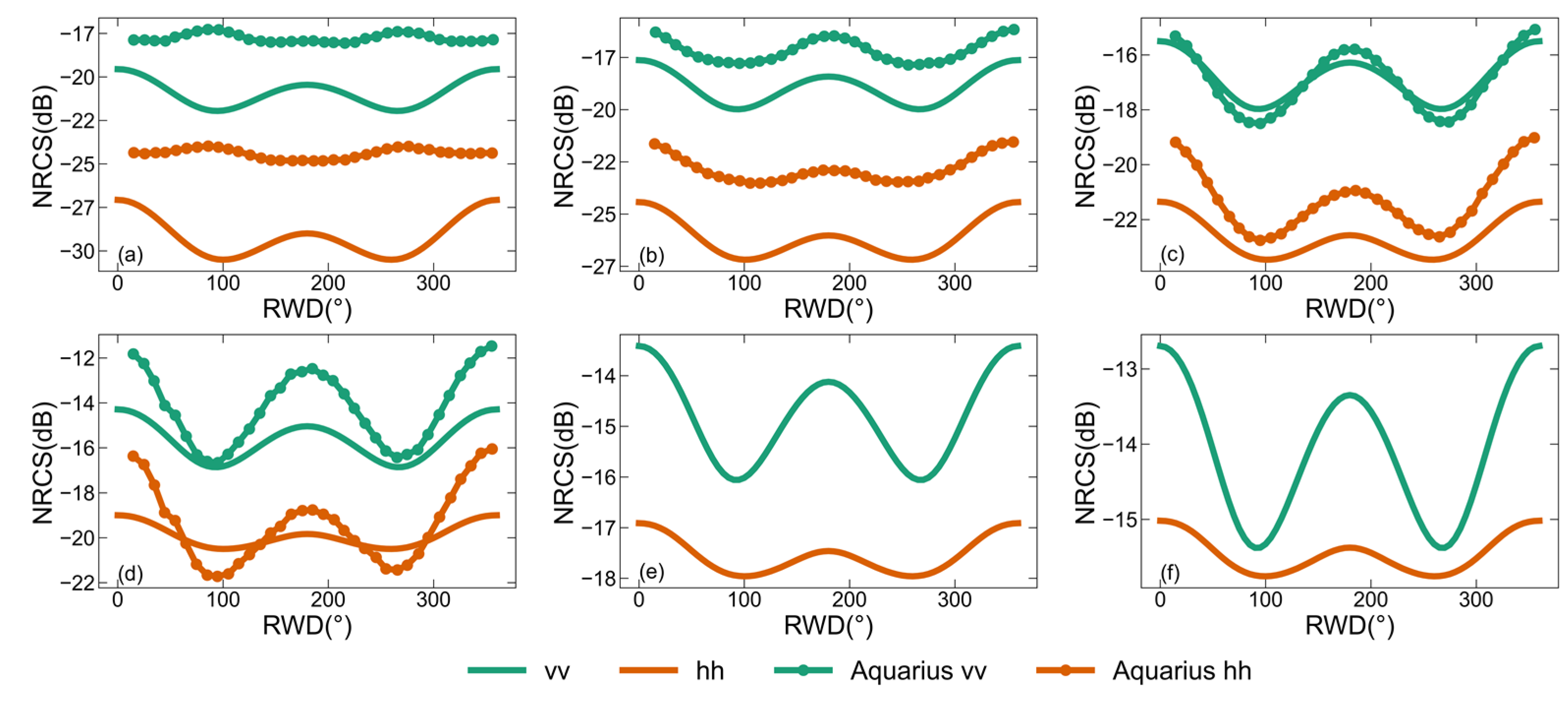
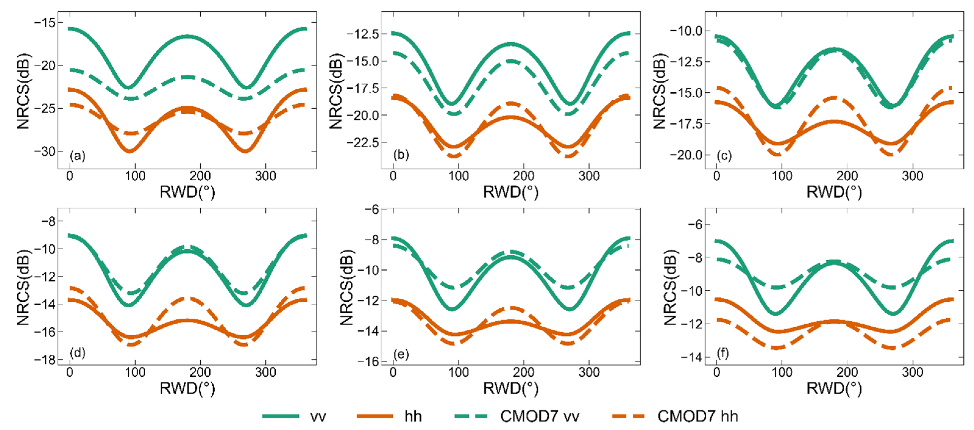
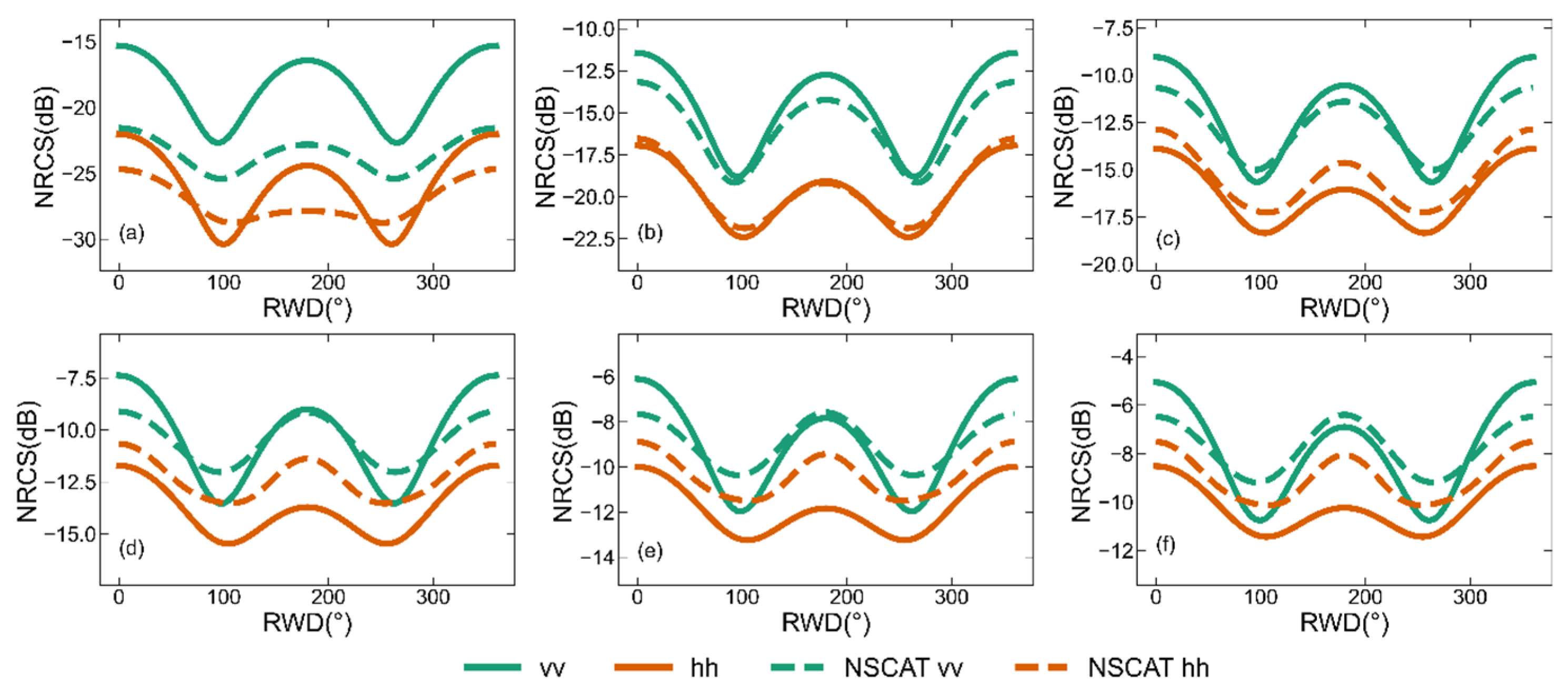
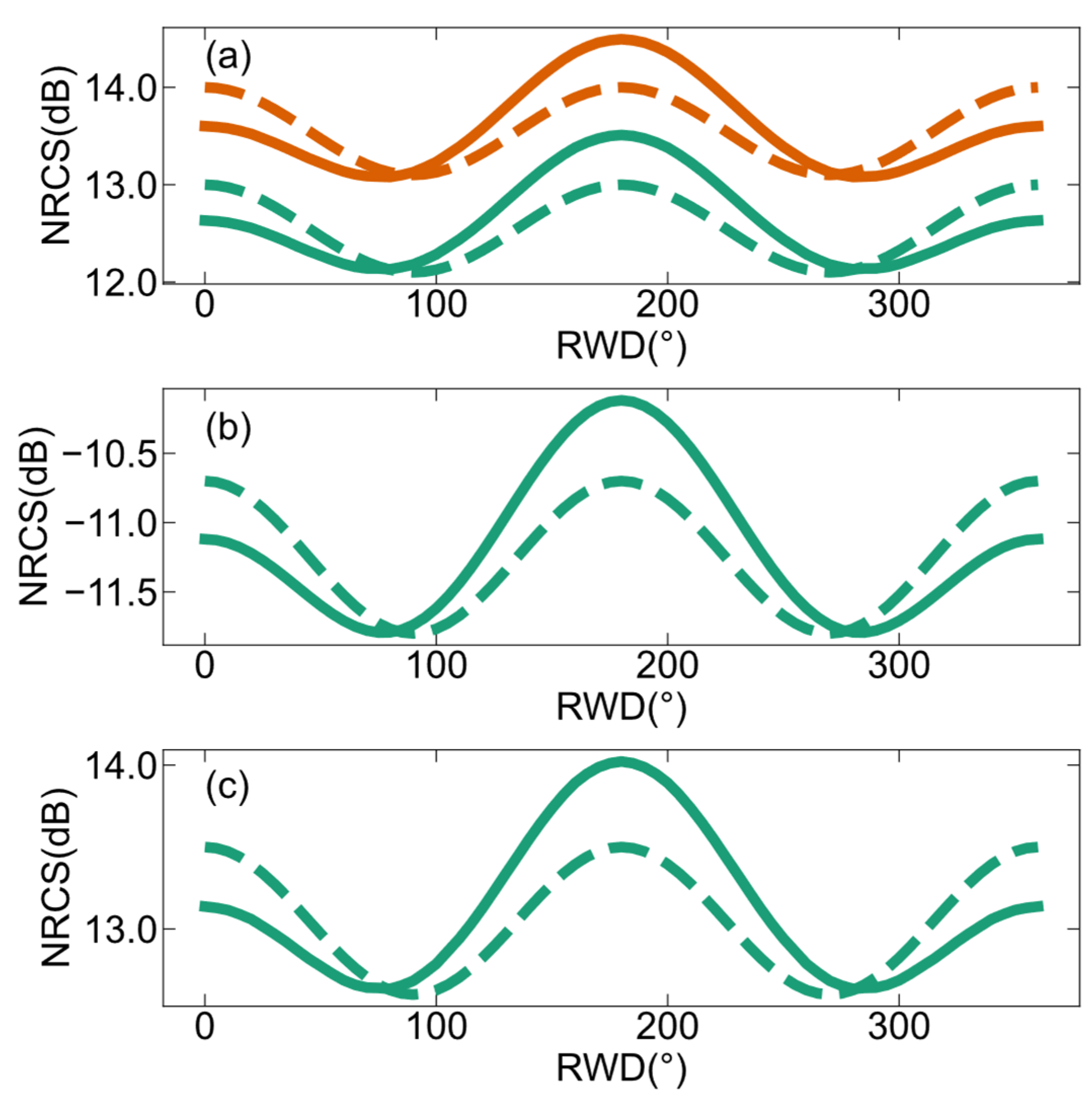
3.1. Numerical Results of Backscattering NRCS

This section analyzes the dependencies of the backscattering NRCSs simulated by the two-scale pBRDF matrix on wind speed, RWD, and incidence zenith angle at different microwave bands. Meanwhile, the simulations are compared with GMFs and a classical two-scale model (TSM), also with experimental data.

Figure 4 demonstrates the dependencies of $vv$-, $hh$-, and $vh$-polarized backscattering NRCSs on RWD at the Ku- and C-band for a 10 m/s wind speed with different ocean wave spectra. The values of $hv$ and $vh$ polarizations are the same, so only the results of $vh$ polarization are shown. Figure 4a–d show that the two-scale pBRDF matrix can reasonably reproduce the dependencies of the $vv$-, $hh$-, and $vh$-polarized backscattering NRCSs on RWD at the Ku- and C-band. They all have $\cos 2\phi$ harmonic variations and positive upwind–crosswind asymmetries.

The simulations of backscattering NRCSs are influenced by not only the electromagnetic scattering model but also the ocean wave spectra. Figure 4 shows simulations of the two-scale pBRDF matrix at the Ku- and C-band using different ocean wave spectra, including Kudryatsev, Elfouhaily, and DV2. For comparisons, the corresponding GMF simulations and experimental data are provided to assess the applicability of the three spectra. The GMFs are NSCAT4 for the Ku-band and CMOD7 for the C-band. The experimental data for the Ku-band are from an airborne scatterometer [42], and those for the C-band are from RADARSAT-2 SAR [43]. Figure 4a illustrates the simulated $vv$- and $hh$-polarized backscattering NRCSs using three different ocean wave spectra at the Ku-band. The most pronounced differences occur in the crosswind direction for two polarizations, and they are about 4 dB for $vv$ and 2 dB for $hh$. In Figure 4a, the experimental data and NSCAT4 simulations are almost identical for both polarizations. Compared to the experimental data and NSCAT4 simulations, the DV2 spectrum makes the two-scale pBRDF matrix have the highest consistency for $vv$ polarization, with the biggest difference measuring less than 0.5 dB. For $hh$ polarization, the Kudryatsev spectrum makes the highest consistencies in the upwind (about 1 dB difference) and downwind directions (no difference), while the Elfouhaily spectrum makes the highest consistency (no difference) in the crosswind direction, with the biggest difference being less than 1 dB. Figure 4b is the $vh$ polarization at the Ku-band. The Elfouhaily spectrum shows a more consistent RWD dependence on the experimental data. Figure 4c illustrates the simulated $vv$- and $hh$-polarized backscattering NRCSs using three different ocean wave spectra at the C-band. There are large differences between the $vv$-polarized backscattering NRCSs of the experimental data and those simulated with CMOD7. CMOD7 only supports simulating the $vv$-polarized backscattering NRCSs. Compared to the CMOD7 simulations, the Kudryatsev spectrum shows the highest consistency overall, except in the crosswind direction, while, compared to the experimental data, the Elfouhaily spectrum has the highest consistency overall. For $hh$ polarization, the Kudryatsev and DV2 spectra are comparable, and they have the highest consistency compared to the experimental data. Figure 4d is the $vh$ polarization at the C-band; the Kudryatsev and DV2 spectra show a more consistent RWD dependence than the Elfouhaily spectrum on the experimental data.

Figure 4 also shows the comparisons of the backscattering NRCSs simulated by the two-scale pBRDF matrix and the classical TSM. The classical TSM simulations are adopted from the literature [37] and do not incorporate hydrodynamic modulation. Compared to the experimental data, the $vv$ polarization at the Ku-band of the classical TSM has the biggest difference of about 2 dB in the crosswind direction, while the $hh$ polarization has the biggest difference of about 4 dB in the upwind direction. The biggest differences for the C-band $vv$ and $hh$ polarizations are 2 dB in the crosswind direction and 2 dB in the upwind direction, respectively. For the $vh$ polarizations at the Ku- and C-band, the differences are about 5 dB overall. When comparing the two-scale pBRDF matrix and the classical TSM simulations, the simulations closest to the experimental data of the two-scale pBRDF matrix are used.

Figure 5 depicts the dependencies of $vv$-, $hh$-, and $vh$-polarized backscattering NRCSs on the incidence zenith angle at the X-band for a 10 m/s wind speed with different RWDs. Figure 5a shows the results at 0° RWD (upwind direction). The $vv$ and $hh$ polarizations are almost identical until the 25° incidence zenith angle, after which the difference between the $vv$ and $hh$ polarizations begins to be significant, with $vv$ polarization being greater than $hh$ polarization. The $vh$ polarization increases first and gradually decreases after 25°. The results at 90° and 180° RWD are shown, respectively, in Figure 5b,c and have the same dependencies on the incidence zenith angle. The $vv$-, $hh$-, and $vh$-polarized backscattering NRCSs exhibit the correct variations with respect to the incidence zenith angle for all three RWDs. At small incidence angles (<25°), the dominant mechanism is the GO. However, for larger incidence angles (>25°), the dominant mechanism shifts to Bragg scattering. Consequently, the difference between $vv$ and $hh$ polarizations becomes evident after 25°. For all three RWDs, the $vh$ polarization increases initially and then decreases. The increase is attributed to the emergence of Bragg scattering, while the subsequent decrease is due to the increase in the incidence zenith angle. Figure 5d shows the polarization ratio (PR) of the two-scale pBRDF matrix as a function of the incidence angle under different azimuth angles. The PR simulations of three X-band PR models are provided [44,45,46]. The three PR models only account for the influence of the incidence angle on the PR, while the PR simulated by the two-scale pBRDF matrix is a function of the incidence zenith angle, RWD, and, perhaps, wind speed. The PRs at three RWD all increase with the incidence zenith angle and are more consistent with the X-PR model, which is derived from TerraSAR-X dual-polarization data.

Figure 6, Figure 7 and Figure 8 depict the dependencies of the $vv$- and $hh$-polarized backscattering NRCSs predicted by the two-scale pBRDF matrix on the wind speed at the L-band, C-band, and Ku-band, respectively, with the Aquarius beam 3 backscatters [47], CMOD7, and NSCAT4 simulations for comparison. The $hh$-polarized backscattering NRCSs of CMOD7 are obtained via $vv$ polarization and the PR model [43]. Figure 6, Figure 7 and Figure 8 show that the $vv$- and $hh$-polarized backscattering NRCSs both increase with the increase in the wind speed and gradually become saturated after 20 m/s. In Figure 6, compared with the Aquarius beam 3 backscatters at 5–20 m/s, the differences are significant, especially for $hh$-polarized backscattering NRCSs. In Figure 7, except for $vv$ polarization at 5 m/s, which has the biggest difference of about 5 dB in the wind direction, the differences in the $vv$ and $hh$ polarization at the C-band are smaller than 2.5 dB. Comparable differences are observed in the Ku-band, in Figure 8.

Figure 6, Figure 7 and Figure 8 also show the dependence of the $vv$- and $hh$-polarized backscattering NRCSs predicted by the two-scale pBRDF matrix on the frequency. The $vv$- and $hh$-polarized backscattering NRCSs increase with the increase in the frequency.

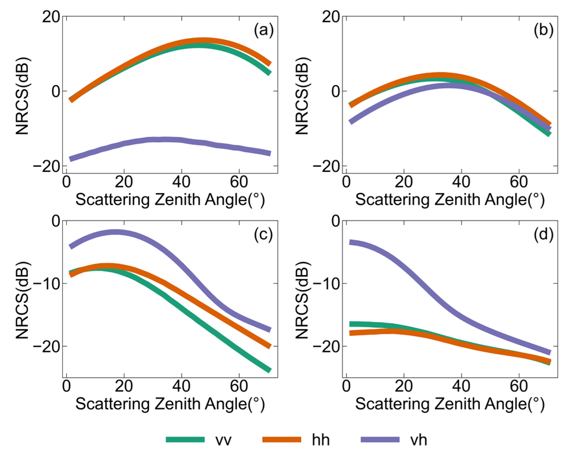
3.2. Numerical Results of Bistatic NRCS

In active remote sensing, the application of bistatic scattering is less than that of backscattering. Bistatic scattering is generally applied to the L-band. Figure 9 illustrates the bistatic-scattering NRCSs for $vv$, $hh$, and $vh$ linear polarizations as a function of the scattering zenith angle at the L-band under a wind speed of 10 m/s, an incidence zenith angle of 45°, and a scattering azimuth angle of 0° for four different scattering zenith angles: 0°, 30°, 60°, and 90°. Figure 9a shows the special case of in-plane forward scattering. The $vv$ and $hh$ polarizations first increase and then decrease with the increase in the scattering zenith angle, with the peak occurring near 45°. However, the peak of $vh$ polarization does not occur near 45°. This is because $vv$ and $hh$ polarizations are influenced by both GO and Bragg scattering, while $vh$ polarizations are solely influenced by Bragg scattering. Comparing the results shown in Figure 9a–d, the $vv$ and $hh$ polarizations decrease with the increase in the scattering azimuth angle ${\phi }^s$. When ${\phi }^s$ is greater than 60°, the $vv$ and $hh$ polarizations are smaller than the $vh$ polarizations. This is due to the transition from in-plane scattering to out-of-plane scattering, where the GO is no longer the dominant factor and can even fail at a large scattering zenith angle.

Figure 10 shows the comparisons of bistatic NRCSs simulated by the two-scale pBRDF matrix and SSA2 at the L-band. The results of SSA2 are adopted from the literature [37] and are derived without hydrodynamic modulation. Figure 10a compares the linear $vv$ and $hh$ polarizations, while Figure 10b,c show ${\sigma }_{RR}^0$ and ${\sigma }_{LR}^0$ circular polarizations, respectively. The differences in the bistatic-scattering NRCSs simulated by SSA2 and the two-scale pBRDF matrix do not exceed 0.5 dB for all three polarization types, and the discrepancies are primarily observed in the upwind and downwind directions. The bistatic-scattering NRCSs have smaller amplitudes over RWD compared to backscattering NRCSs.

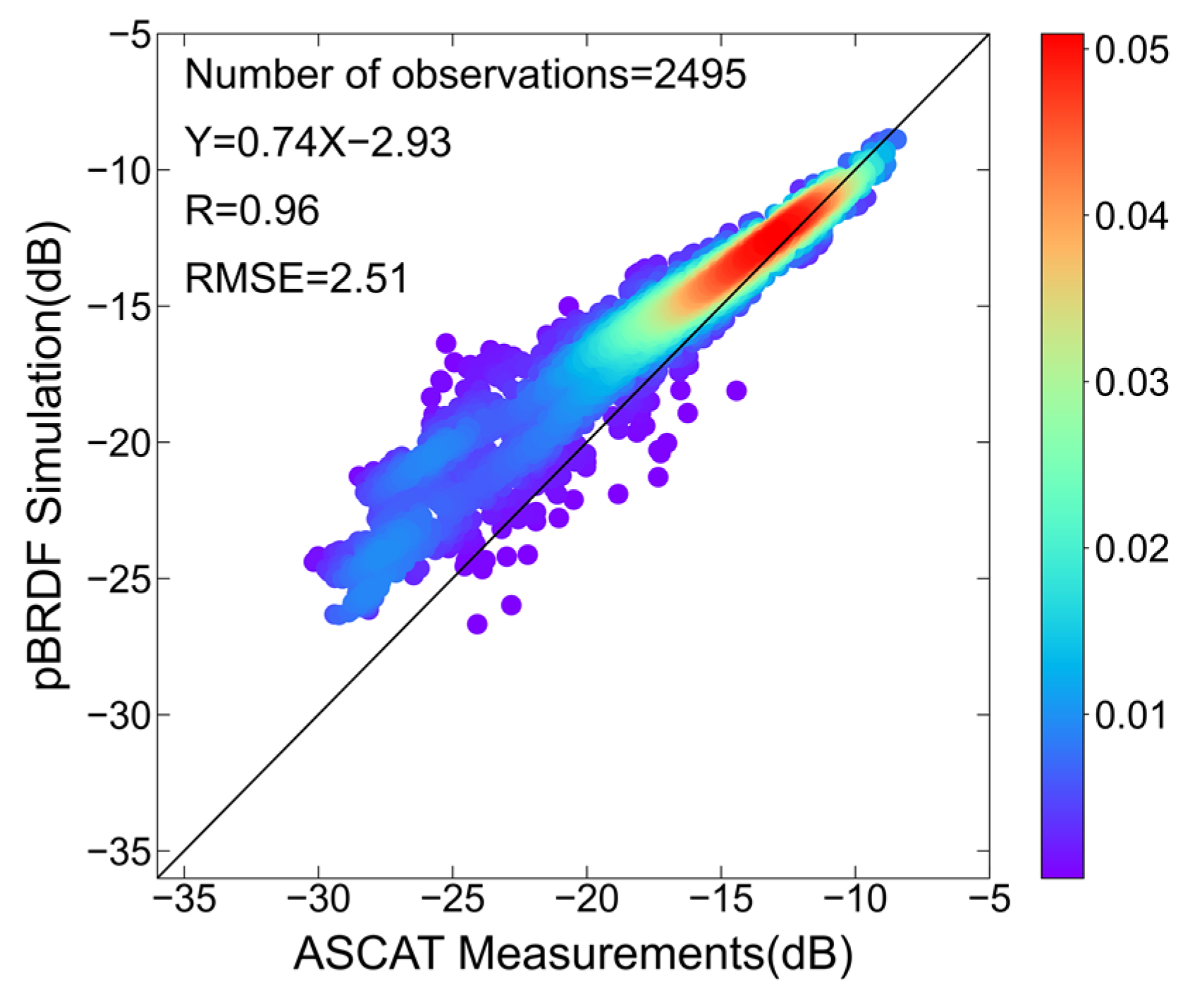
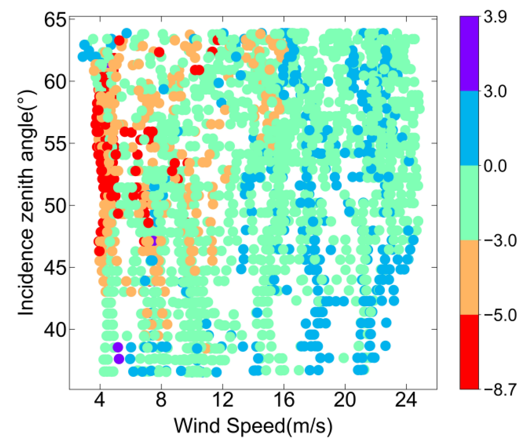
3.3. Comparison with MetOP-C ASCAT Scatterometer

The validation of the two-scale pBRDF matrix for active remote sensing was conducted by comparing the simulations with measurements of spaceborne microwave active sensors. The datasets used for the comparisons included satellite observations, the simulations produced by the two-scale pBRDF matrix, and auxiliary datasets. The MetOP-C ASCAT scatterometer operating at the C-band was chosen for validating the backscatter. The ASCAT observations were collocated with surface parameters from the European Centre for Medium-Range Weather Forecasts (ECMWF) Re-Analysis (ERA)-Interim and the Mercator Ocean reanalysis. Surface-level parameters such as SST, wind speed, and wind direction were extracted from the ECMWF ERA-interim at a spatial resolution of 0.25°. The SSS data were derived from the Mercator Ocean reanalysis at a spatial resolution of 0.083°. Additionally, total precipitation and sea ice percentage data from the ERA-interim were used for quality control. The collocation between the auxiliary datasets and satellite data was performed using the near-neighbor interpolation scheme, with a temporal difference of no more than 1 h.

Figure 11 shows the linear regression of backscattering NRCSs between simulations of the two-scale pBRDF matrix and the measurements of ASCAT. The correlation coefficient is 0.9634, and the RMSE is 2.5083 dB. There exists a strong linear relationship between the simulations and the measurements. However, the two-scale pBRDF matrix tends to overestimate the NRCSs in the low NRCS region where the simulations correspond to small wind speeds or/and large incidence zenith angles. Figure 12 depicts a two-dimensional scatterplot illustrating the differences between the measurements and the simulations as a function of wind speed and incidence zenith angle. The majority of points fall within the range of ±3 dB. The largest difference observed is −8.7 dB, which occurs at low wind speeds and large incidence zenith angles.

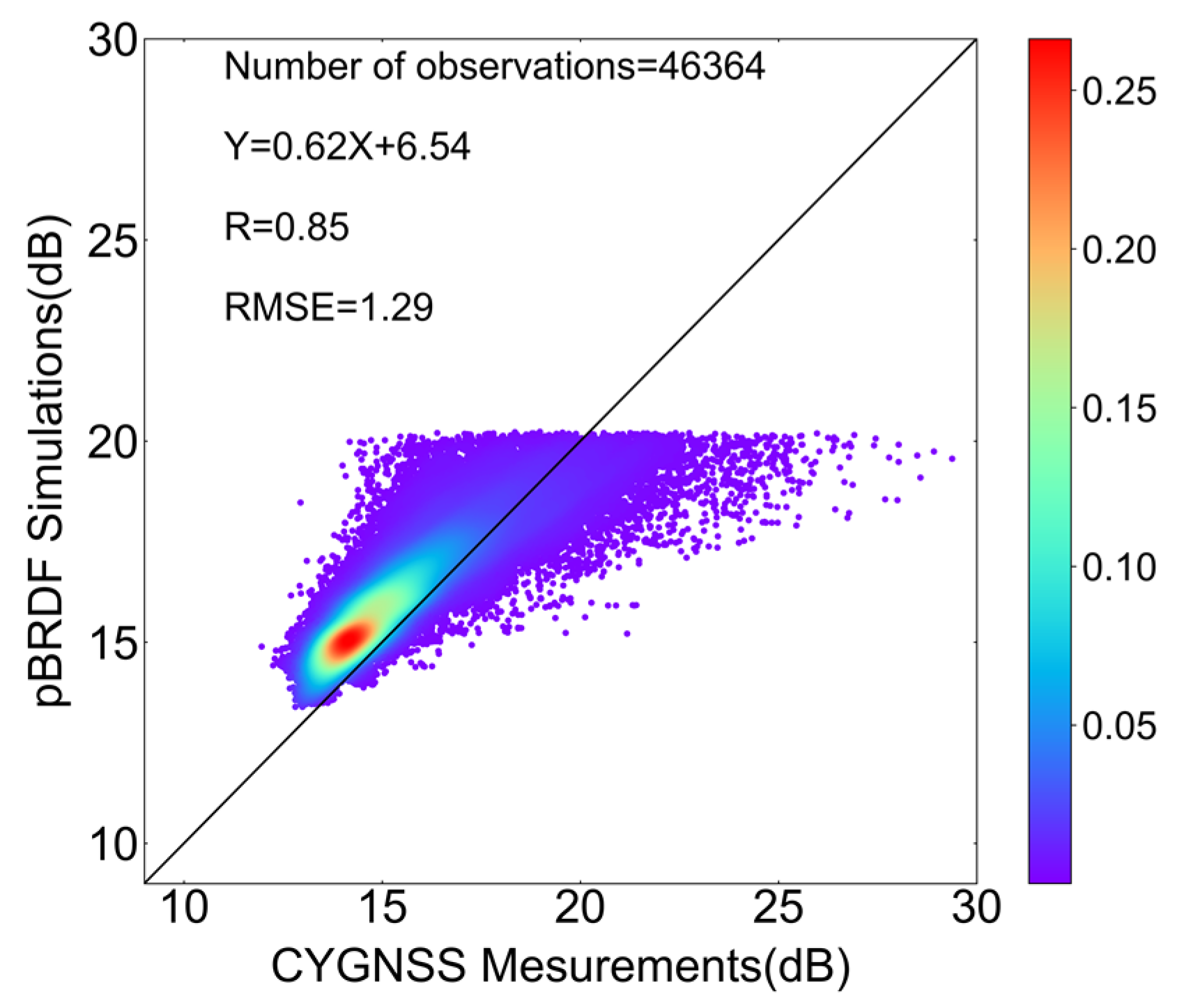
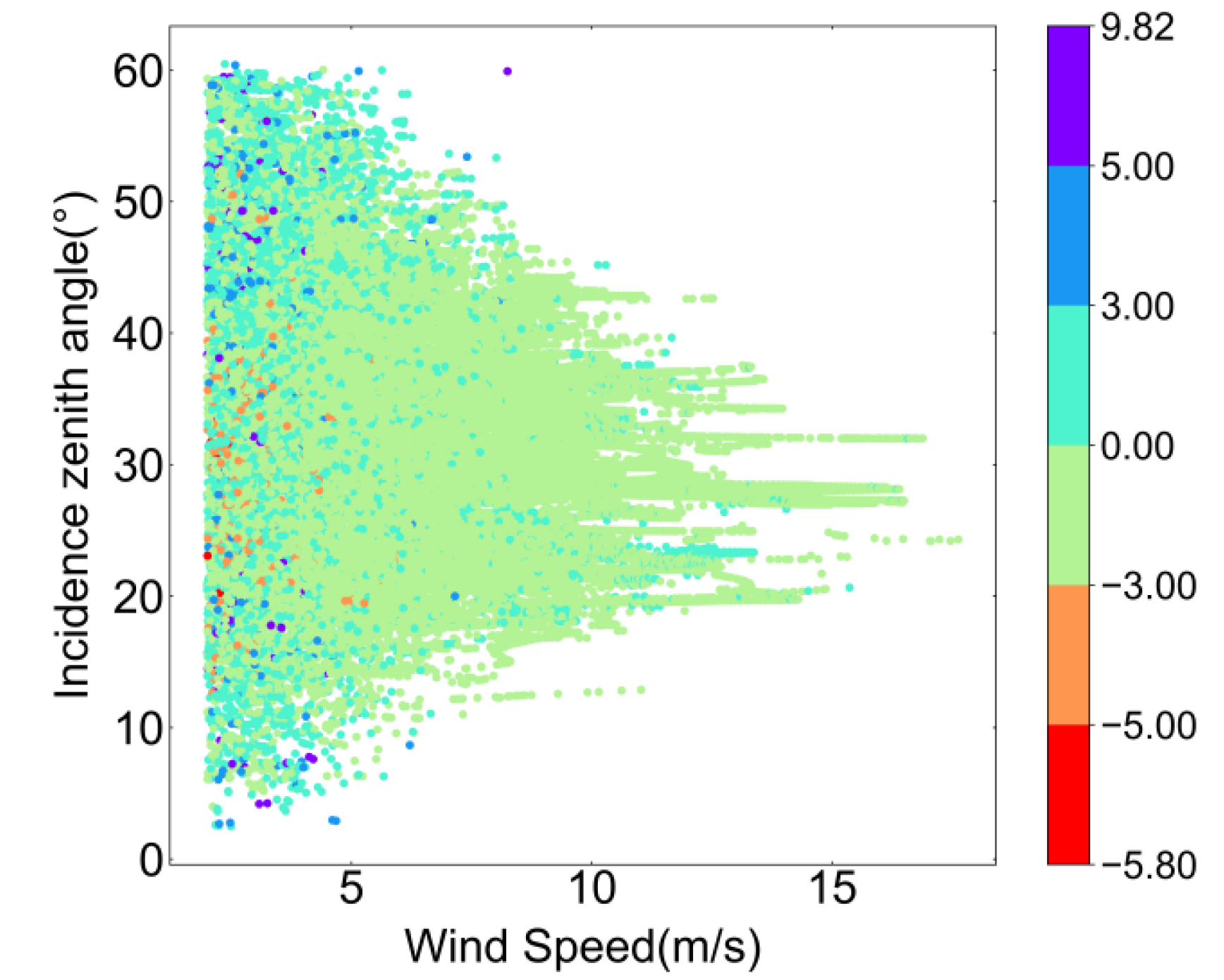
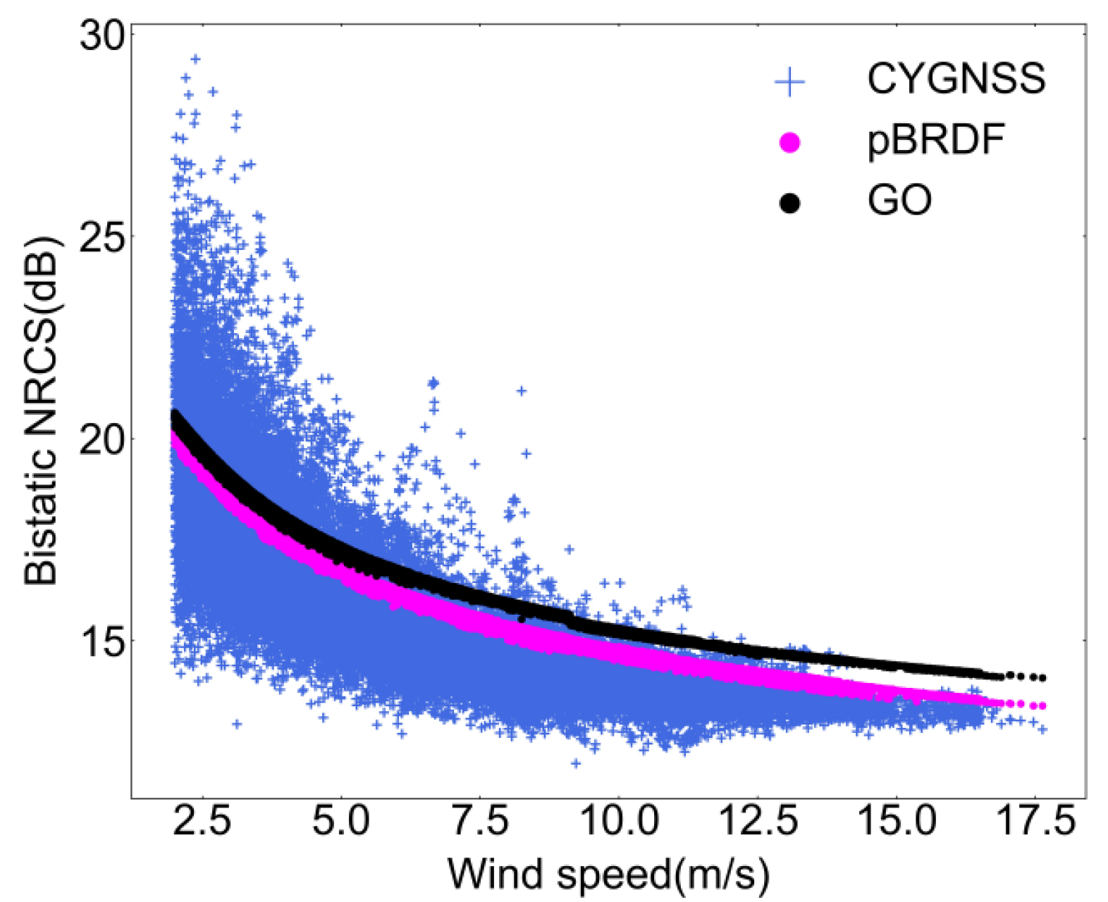
3.4. Comparison with CYGNSS Reflectometry

The validation of the two-scale pBRDF matrix for bistatic-scattering NRCSs is conducted by comparison with the measurements of CYGNSS reflectometry. The CYGNSS is an eight-satellite constellation intended to use ocean wind data from GNSS-R to improve the tracking and intensity forecasting of tropical cyclones. It offers high spatial and temporal resolutions and operates at the L-band, which experiences lower rain attenuation compared to other frequencies [48]. CYGNSS observes the ocean surface using forward scattering, and the physical GMF used for deriving the observables is the GO model, which is valid under specific conditions. Limited research has been conducted on using a two-scale GMF for GNSS reflectometry simulations. The CYGNSS Level 1b data product contains the bistatic NRCS in a circular polarization ${\sigma }_{LR}^0$, generated from delay-Doppler mapping by removing the effect of satellite attitudes, direct power, and antenna gain [49]. The signal-to-noise ratio of the measurements used for these comparisons needs to be greater than 6.

Figure 13 presents the linear regression of circularly polarized bistatic NRCSs between simulations of the two-scale pBRDF matrix and measurements of CYGNSS. A cut exists around 20 dB, as data with wind speeds less than 2 m/s were excluded. The correlation coefficient is 0.8480, and the RMSE is 1.2859 dB. The discrete points are primarily concentrated in cases with large signals. Forward scattering differs from backscattering in that it relies on large-scale reflections, and, as the wind speed decreases, the signal strength tends to increase. Figure 14 is a two-dimensional scatterplot showing the differences between the CYGNSS measurements and the two-scale pBRDF matrix simulations as a function of wind speed and incidence zenith angle. The findings align with the ASCAT simulation case. The majority of the differences are smaller than 3 dB, while larger differences occur at low wind speeds.

Figure 15 shows a plot of circularly polarized bistatic NRCSs versus wind speed. The bistatic NRCSs come from CYGNSS measurements, the two-scale pBRDF matrix, and GO simulations. Compared with the GO model, the two-scale pBRDF matrix shows a higher consistency with the CYGNSS measurements, especially at higher wind speeds, which indicates that the two-scale pBRDF matrix may have a better performance in DDM simulations and wind speed recording.

4. Discussion

The main objectives of this study were twofold: first, to evaluate whether the two-scale pBRDF matrix model could reasonably characterize the dependency between the NRCS and the ocean surface parameters, and second, to assess its applicability to different active payloads. In pursuit of these objectives, we conducted systematic numerical simulations of NRCSs using the two-scale pBRDF matrix and compared the simulations with observations from spaceborne active sensors.

In this study, numerical simulations were conducted within the wind speed range of 0–30 m/s, an RWD range of 0–360°, an incidence zenith angle range of 0–70°, and across different bands (L-, C-, X-, and Ku-band), and they were compared with simulations provided by GMFs and experimental data. The results indicate that the two-scale pBRDF matrix can reasonably characterize the dependency of polarized backscatter on wind speed, wind direction, incidence angle, and frequency. However, the simulation accuracy of the two-scale pBRDF matrix is not always reliable. Using the DV2 ocean wave spectrum, there was a significant underestimation of the $vv$- and $hh$-polarized backscatter at the L-band when the wind speed was less than 10 m/s, and overestimations of the $vv$-polarized backscatter at the C-band and Ku-band occurred at a 5 m/s wind speed. A 2 dB underestimation of the $hh$-polarized backscatter at the Ku-band occurred in the downwind direction when the wind speed exceeded 20 m/s. Figure 4a shows that using different ocean wave spectra introduces approximately a 4 dB difference for $vv$ polarization in the crosswind direction, indicating a significant impact of the ocean wave spectrum on the simulations of the two-scale pBRDF matrix. The suitability of ocean wave spectra varies with the wind speeds and incidence zenith angles. Further research is needed regarding the selection of the ocean wave spectra for the two-scale pBRDF matrix.

The overestimation of the two-scale pBRDF matrix model under low wind speed conditions was also evident in the comparisons with satellite observations. At very low wind conditions, the ocean surface is heavily influenced by swell and ocean waves, which are less correlated to the local wind. The ocean surface roughness is sensitive not only to the short waves driven by the local wind but also to the long waves generated by nonlocal swell. In the cases of medium-to-high wind speeds, the local wind dominates, and the effect of swell can be disregarded. However, at wind speeds below 5 m/s, the local wind is weak, and the presence of swell becomes evident [50,51,52].

Some L-band observations suggested that radar backscatter signals near a wind speed of 5 m/s exhibited a negative upwind–downwind asymmetry, whereas the simulation of the two-scale pBRDF matrix displayed a positive upwind–downwind asymmetry. This difference arises from the positive upwind–crosswind asymmetry produced by the Bragg scattering mechanism used in two-scale sea surface scattering models, with the pBRDF matrix essentially being a two-scale model.

While the two-scale pBRDF matrix still presents the aforementioned shortcomings in its application, these issues are not insurmountable. In the future, we will focus on addressing these problems to further optimize the model, enabling the two-scale pBRDF matrix to be more effectively utilized in microwave active remote sensing. Despite its limitations, the two-scale pBRDF matrix also has notable strengths, such as the ability to simultaneously simulate linearly polarized, backscatter, and bistatic scattering, as well as circularly polarized signals. Additionally, the two-scale pBRDF matrix exhibits capabilities for passive remote sensing applications. It can consistently simulate both active and passive remote sensing signals over the ocean surface, facilitating the joint utilization of various types of microwave active and passive payloads.

5. Conclusions

In this study, starting from the concepts, the relationships between NRCSs and the two-scale pBRDF matrix elements were derived. The application of the two-scale pBRDF matrix developed for fully polarized ocean–atmosphere-coupled radiative transfer was expanded from passive remote sensing to active remote sensing. Comprehensive numerical simulations across the L-, C-, X-, and Ku-bands were carried out, and these simulations were compared with experimental data from the literature, simulations of GMFs, and classical electromagnetic scattering models such as TSM and SSA2. For further validation, the backscattering and bistatic-scattering simulations of the two-scale pBRDF matrix were compared with measurements from the ASCAT and CYGNSS, respectively.

The two-scale pBRDF matrix demonstrated reasonable dependencies in terms of ocean surface wind speeds, wind direction (RWD), geometries, and frequencies. The comparisons with the GMFs and experimental data affirmed the reliable accuracy of the two-scale pBRDF matrix in simulating backscattering NRCSs at the C-, X-, and Ku-band, except for cases at a low wind speed (<5 m/s) and horizontally polarized NRCSs at the Ku-band and at a high wind speed (>20 m/s). The comparison of bistatic NRCSs with SSA2 showed a high performance for simulating bistatic-scattering NRCSs.

The linear regression of the backscattering NRCSs from the simulations of the two-scale pBRDF matrix and the measurements of ASCAT demonstrated a correlation coefficient of 0.9634 and an RMSE of 2.5083 dB. Large differences between the simulations and the measurements were observed at low wind speeds, where the effects of swell and nonlocal waves were prominent. For medium-to-high wind speeds, the two-scale pBRDF matrix exhibited a good performance in simulating NRCSs. When compared with the CYGNSS measurements, the linear regression of circularly polarized bistatic NRCSs demonstrated a correlation coefficient of 0.8480 and an RMSE of 1.2859 dB. The comparison between the two-scale pBRDF matrix and GO highlighted that the two-scale pBRDF matrix had a better performance in simulating bistatic NRCSs, especially at high wind speeds (>5 m/s).

In conclusion, the two-scale pBRDF matrix demonstrated a high level of confidence in modeling backscattering and bistatic NRCSs for active sensor applications, although there remained some challenges. Its versatility as a unified physical electromagnetic scattering model for both active and passive remote sensing was demonstrated. The ultimate goal of this study was to establish a consistent approach for retrieving atmospheric and surface parameters using both passive and active measurements.

References

1. Alerskans, E.; Zinck, A.S.P.; Nielsen-Englyst, P.; Høyer, J.L. Exploring machine learning techniques to retrieve sea surface temperatures from passive microwave measurements. Remote Sens. Environ. 2022, 281, 113–220. [Google Scholar] [CrossRef]
2. Chi, J.; Kim, H.C. Retrieval of daily sea ice thickness from AMSR2 passive microwave data using ensemble convolutional neural networks. GISci. Remote Sens. 2021, 58, 812–830. [Google Scholar] [CrossRef]
3. Le Vine, D.M.; Dinnat, E.P. The Multifrequency Future for Remote Sensing of Sea Surface Salinity from Space. Remote Sens. 2020, 12, 1381. [Google Scholar] [CrossRef]
4. Pospelov, M.N. Surface wind speed retrieval using passive microwave polarimetry: The dependence on atmospheric stability. IEEE Trans. Geosci. Remote Sens. 1996, 34, 1166–1171. [Google Scholar] [CrossRef]
5. Weng, F.; Grody, N.C. Retrieval of cloud liquid water using the special sensor microwave imager (SSM/I). J. Geophys. Res. Atmos. 1994, 99, 25535–25551. [Google Scholar]
6. Tian, Y.; Wen, B.; Zhou, H.; Wang, C.; Yang, J.; Huang, W. Wave Height Estimation from First-Order Backscatter of a Dual-Frequency High Frequency Radar. Remote Sens. 2017, 9, 1186. [Google Scholar] [CrossRef]
7. Yang, J.; Zhang, J.; Jia, Y.; Fan, C.; Cui, W. Validation of Sentinel-3A/3B and Jason-3 Altimeter Wind Speeds and Significant Wave Heights Using Buoy and ASCAT Data. Remote Sens. 2020, 12, 2079. [Google Scholar] [CrossRef]
8. Yu, P.; Xu, W.X.; Zhong, X.J.; Johannessen, J.A.; Yan, X.H.; Geng, X.P.; He, Y.R.; Lu, W.F. A Neural Network Method for Retrieving Sea Surface Wind Speed for C-Band SAR. Remote Sens. 2022, 14, 2269. [Google Scholar] [CrossRef]
9. Robitaille, P.M. On the validity of Kirchhoff’s law of thermal emission. IEEE Trans. Plasma Sci. 2003, 31, 1263–1267. [Google Scholar] [CrossRef]
10. Veysoglu, M.E.; Yueh, H.A.; Shin, R.T.; Kong, J.A. Polarimetric Passive Remote Sensing of Periodic Surfaces. J. Electromagn. Waves Appl. 1991, 5, 267–280. [Google Scholar] [CrossRef]
11. Yueh, S.H.; Kwok, R. Electromagnetic fluctuations for anisotropic media and the generalized Kirchhoff’s law. Radio Sci. 1993, 28, 471–480. [Google Scholar] [CrossRef]
12. Priest, R.; Meier, S. Polarimetric microfacet scattering theory with applications to absorptive and reflective surfaces. Opt. Eng. 2002, 41, 988–993. [Google Scholar] [CrossRef]
13. Hyde, M.W.; Schmidt, J.D.; Havrilla, M.J. A geometrical optics polarimetric bidirectional reflectance distribution function for dielectric and metallic surfaces. Opt. Express 2009, 17, 22138–22153. [Google Scholar] [CrossRef] [PubMed]
14. Diner, D.J.; Xu, F.; Martonchik, J.V.; Rheingans, B.E.; Geier, S.; Jovanovic, V.M.; Davis, A.; Chipman, R.A.; McClain, S.C. Exploration of a Polarized Surface Bidirectional Reflectance Model Using the Ground-Based Multiangle SpectroPolarimetric Imager. Atmosphere 2012, 3, 591–619. [Google Scholar] [CrossRef]
15. Boukabara, S.A.; Eymard, L.; Guillou, C.; Lemaire, D.; Sobieski, P.; Guissard, A. Development of a modified two-scale electromagnetic model simulating both active and passive microwave measurements: Comparison to data remotely sensed over the ocean. Radio Sci. 2002, 37, 1–11. [Google Scholar] [CrossRef]
16. Sobieski, P.; Guissard, A.; Baufays, C. Synergic inversion technique for active and passive microwave remote sensing of the ocean. IEEE Trans. Geosci. Remote Sens. 1991, 29, 391–406. [Google Scholar] [CrossRef]
17. English, S.; Prigent, C.; Johnson, B.; Yueh, S.; Dinnat, E.; Boutin, J.; Newman, S.; Anguelova, M.; Meissner, T.; Kazumori, M.; et al. Reference-Quality Emission and Backscatter Modeling for the Ocean. Bull. Am. Meteorol. Soc. 2020, 101, E1593–E1601. [Google Scholar] [CrossRef]
18. He, L.; Weng, F. Improved Microwave Ocean Emissivity and Reflectivity Models Derived from Two-Scale Roughness Theory. Adv. At. Sci. 2023, 40, 1923–1938. [Google Scholar] [CrossRef]
19. Guo, L.X.; Guo, X.Y.; Zhang, L.B. Bidirectional reflectance distribution function modeling of one-dimensional rough surface in the microwave band. Chin. Phys. B 2014, 23, 114102. [Google Scholar] [CrossRef]
20. David, L.; Fawwaz, U. Microwave Radar and Radiometric Remote Sensing; Artech: Morristown, NJ, USA, 2015; Volume 1. [Google Scholar]
21. Bettenhausen, M.H.; Smith, C.K.; Bevilacqua, R.M.; Wang, N.Y.; Gaiser, P.W.; Cox, S. A nonlinear optimization algorithm for WindSat wind vector retrievals. IEEE Trans. Geosci. Remote Sens. 2006, 44, 597–610. [Google Scholar] [CrossRef]
22. Dinnat, E.P.; Boutin, J.; Caudal, G.; Etcheto, J.; Waldteufel, P. Influence of sea surface emissivity model parameters at L-band for the estimation of salinity. Int. J. Remote Sens. 2002, 23, 5117–5122. [Google Scholar] [CrossRef]
23. Johnson, J.; Theunissen, W.H.; Ellingson, S.W. A Study of Sea Emission Models for WindSAT. In Proceedings of the IGARSS ’03—2003 IEEE International Geoscience and Remote Sensing Symposium, Toulouse, France, 21–25 July 2003; pp. 717–719. [Google Scholar]
24. Lyzenga, D.R.; Vesecky, J.F. Two-Scale Polarimetric Emissivity Model: Efficiency Improvements and Comparisons with Data. Prog. Electromagn. Res. 2002, 37, 205–219. [Google Scholar] [CrossRef]
25. Pierdicca, N.; Marzano, F.S.; Guerriero, L.; Pampaloni, P. On the Effect of Atmospheric Emission Upon the Passive Microwave Polarimetric Response of an Azimuthally Anisotropic Sea Surface. J. Electromagn. Waves Appl. 2000, 14, 355–358. [Google Scholar] [CrossRef]
26. Yueh, S.H.; Nghiem, S.V.; Kwok, R. Comparison of a polarimetric scattering and emission model with ocean backscatter and brightness measurements. In Proceedings of the IGARSS ’94—1994 IEEE International Geoscience and Remote Sensing Symposium, Pasadena, CA, USA, 8–12 August 1994; Volume 1, pp. 258–260. [Google Scholar]
27. Anderson, R. Matrix description of radiometric quantities. Appl. Opt. 1991, 30, 858–867. [Google Scholar] [CrossRef] [PubMed]
28. Flynn, D.S.; Alexander, C.J.O.E. Polarized surface scattering expressed in terms of a bidirectional reflectance distribution function matrix. Opt. Eng. 1995, 34, 1646–1650. [Google Scholar]
29. Sun, Y. Statistical ray method for deriving reflection models of rough surfaces. J. Opt. Soc. Am. 2007, 24, 724–744. [Google Scholar] [CrossRef] [PubMed]
30. Torrance, K.E.; Sparrow, E.M. Theory for Off-Specular Reflection from Roughened Surfaces*. J. Opt. Soc. Am. 1967, 57, 1105–1114. [Google Scholar] [CrossRef]
31. Mobley, C.D. Light and Water: Radiative Transfer in Natural Waters; American Meteorological Society: Boston, MA, USA, 1994. [Google Scholar]
32. Hapke, B. Theory of Reflectance and Emittance Spectroscopy, 2nd ed.; Cambridge University Press: Cambridge, UK, 2012. [Google Scholar]
33. Kazumori, M.; English, S.J. Use of the ocean surface wind direction signal in microwave radiance assimilation. Q. J. R. Meteorol. Soc. 2014, 141, 1354–1375. [Google Scholar] [CrossRef]
34. Kilic, L.; Prigent, C.; Jimenez, C.; Turner, E.; Hocking, J.; English, S.; Thomas, M.; Emmanuel, D. Development of the SURface Fast Emissivity Model for Ocean (SURFEM-Ocean) Based on the PARMIO Radiative Transfer Model. Earth Space Sci. 2023, 10, 11. [Google Scholar] [CrossRef]
35. Saunders, R.; Brunel, P.; English, S.; Bauer, P.; O’Keeffe, U.; Francis, P.; Rayer, P. RTTOV-8-Science and Validation Report; Met Office Forecasting and Research Technical Document (Technical Report No. NWPSAF-MO-TV-007); EUMETSAT: Darmstadt, Germany, 2006. [Google Scholar]
36. Lee, J.S.; Pottier, E. Polarimetric Radar Imaging: From Basics to Applications; CRC Press: Boca Raton, FL, USA, 2009. [Google Scholar]
37. Voronovich, A.G.; Zavorotny, V.U. Full-Polarization Modeling of Monostatic and Bistatic Radar Scattering from a Rough Sea Surface. IEEE Trans. Antennas Propag. 2014, 62, 3. [Google Scholar] [CrossRef]
38. Liu, Q.; Weng, F.; English, S.J. An Improved Fast Microwave Water Emissivity Model. IEEE Trans. Geosci. Remote Sens. 2011, 49, 1238–1250. [Google Scholar] [CrossRef]
39. Stogryn, A. The emissivity of sea foam at microwave frequencies. J. Geophys. Res. (1896–1977) 1972, 77, 1658–1666. [Google Scholar] [CrossRef]
40. Monahan, E.C.; O‘Muircheartaigh, I.G. Whitecaps and the passive remote sensing of the ocean surface. Int. J. Remote Sens. 1986, 7, 627–642. [Google Scholar] [CrossRef]
41. Yueh, S.H. Modeling of wind direction signals in polarimetric sea surface brightness temperatures. IEEE Trans. Geosci. Remote Sens. 1997, 35, 1400–1418. [Google Scholar] [CrossRef]
42. Yueh, S.H.; Wilson, W.J.; Dinardo, S. Polarimetric radar remote sensing of ocean surface wind. IEEE Trans. Geosci. Remote Sens. 2002, 40, 793–800. [Google Scholar] [CrossRef]
43. Zhang, B.; Perrie, W.; Vachon, P.; Li, X.; Pichel, W.; Guo, J.; He, Y. Ocean Vector Winds Retrieval from C-Band Fully Polarimetric SAR Measurements. IEEE Trans. Geosci. Remote Sens. 2012, 50, 4252–4261. [Google Scholar] [CrossRef]
44. Donald, J.H.; Thompson, R.; Mouche, A.; Winstead, S.; Sterner, R.; Monaldo, M. Comparison of high-resolution wind fields extracted from TerraSAR-X SAR imagery with predictions from the WRF mesoscale model. J. Geophys. Res. 2012, 117, c2. [Google Scholar]
45. Elfouhaily, T.; Thompson, D.R.; Vandemark, D.; Chapron, B. A New Bistatic Model for Electromagnetic Scattering from Perfectly Conducting Random Surfaces. Waves Random Media 2001, 9, 33–43. [Google Scholar] [CrossRef]
46. Shao, W.; Li, X.; Lehner, S.; Guanc, C. Development of polarization ratio model for sea surface wind field retrieval from TerraSAR-X HH polarization data. Int. J. Remote Sens. 2014, 35, 11–12. [Google Scholar] [CrossRef]
47. Yueh, S.H.; Tang, W.Q.; Fore, G.; Alexander, F.; Neumann, G.; Hayashi, A.; Freedman, A.; Chaubell, J.; Lagerloef, G. L-Band Passive and Active Microwave Geophysical Model Functions of Ocean Surface Winds and Applications to Aquarius Retrieval. IEEE Trans. Geosci. Remote Sens. 2013, 51, 4619–4632. [Google Scholar] [CrossRef]
48. Ruf, C.; Lyons, A.; Unwin, M.; Dickinson, J.; Rose, R.; Rose, D.; Vincent, M. CYGNSS: Enabling the Future of Hurricane Prediction [Remote Sensing Satellites]. IEEE Geosci. Remote Sens. Mag. 2013, 1, 52–67. [Google Scholar] [CrossRef]
49. Gleason, S.T.; Ruf, C.S.; Clarizia, M.P.; O‘Brien, A.J. Calibration and Unwrapping of the Normalized Scattering Cross Section for the Cyclone Global Navigation Satellite System. IEEE Trans. Geosci. Remote Sens. 2016, 54, 2495–2509. [Google Scholar] [CrossRef]
50. Clarizia, M.P. Investigating the Effect of Ocean Waves on GNSS-R Microwave Remote Sensing Measurements. Ph.D. Thesis, University of Southampton, Southampton, UK, 2012; 219p. [Google Scholar]
51. Huang, F.; Garrison, J.; Leidner, S.; Annane, B.; Hoffman, R.; Giuseppe, G.; Stoffelen, A. A Forward Model for Data Assimilation of GNSS Ocean Reflectometry Delay-Doppler Maps. IEEE Trans. Geosci. Remote Sens. 2021, 59, 2643–2656. [Google Scholar] [CrossRef]
52. Miranda, J.; Vall-llossera, M.; Camps, A.; Duffo, N. Sea surface emissivity at L-band: Swell effects. IEEE Int. Geosci. Remote Sens. Symp. 2002, 5, 2623–2625. [Google Scholar]
Figure 1. Different geometrical configurations for wave scattering from the ocean surface. I i is the incoming radiance vectors from the solid angle d Ω i incident from the ( θ i , φ i ) direction on a microfacet (pink area). I s is the outgoing radiance vectors from the solid angle d Ω s in the ( θ s , φ s ) direction.
Remotesensing 16 01551 g001
Figure 2. The spatial distribution of the scattering energy simulated by the two-scale pBRDF matrix at 37 GHz and 10 m/s wind speed in the specular direction. The unit of each matrix element is sr−1. The SST is 285 K, the SSS is 35‰, and the ocean wave spectrum is the modified Durden and Vesecky spectrum (DV2). (a) Rvvvv, (b) Rvhvh, (c) Re(Rvhvv), (d) Im(Rvhvv), (e) Rhvhv, (f) Rhhhh, (g) Re(Rhhhv), (h) Im(Rhhhv), (i) 2Re(Rvvhv), (j) 2Re(Rvhhh), (k) Re(Rvvhh+Rvhhv), (l) Im(Rhhvv+Rhvvh), (m) 2Im(Rvvhv), (n) 2Im(Rvhhh), (o) Im(Rvvhh+Rvhhv), (p) Re(Rhhvv-Rhvvh).
Remotesensing 16 01551 g002
Figure 3. Comparison of three different emissivity models. The ordinate is the emissivity of each component. The wind speed is 10 m/s, the SST is 285 K, the frequency is 37 GHz, the observation angle is 45°, the SSS is 35‰, and the ocean wave spectrum is DV2. (a) vertical component, (b) horizontal component, (c) the third component, (d) the fourth component.
Remotesensing 16 01551 g003
Figure 4. The dependencies of the backscattering NRCSs predicted by the two-scale pBRDF matrix on RWD at a 10 m/s wind speed and the comparisons with other simulations or data. (a) Simulations of v v (solid line) and h h (dotted line) polarizations at the Ku-band. (b) Simulations of v h polarizations at the Ku-band. (c) Simulations of v v (solid line) and h h (dotted line) polarizations at the C-band. (d) Simulations of v h polarizations at the C-band. The Ku-band and C-band simulations are at incidence zenith angles of 45° and 35°, respectively. The black dots’ line, stars’ line, and triangles’ line are the v v , h h , and v h experimental data, respectively. The SSS is set to 35‰, and the SST is 285 K. The cyan, orange color, and purple colors represent the simulations of the two-scale pBRDF matrix with Kudryatsev, Elfouhaily, and DV2 spectra, respectively. The yellow color represents the classical TSM simulation. The magenta and green colors represent the simulations of the NSCAT4 and CMOD7 simulations, respectively.
Remotesensing 16 01551 g004
Figure 5. The dependencies of the backscattering NRCSs predicted by the two-scale pBRDF matrix on the incidence angle at the X-band and a 10 m/s wind speed. The results are shown for three different RWDs: (a) RWD = 0°, (b) RWD = 90°, and (c) RWD = 180°. (d) The polarization ratios under different RWDs and the comparisons with other X-band polarization ratio models. The SSS is set to 35‰, the SST is 285 K, and the ocean wave spectrum is DV2.
Remotesensing 16 01551 g005
Figure 6. The dependencies of the backscattering NRCSs predicted by the two-scale pBRDF matrix on the wind speed at the L-band. The incidence zenith angle is set to 46°, the SSS is set to 35‰, the SST is 285 K, and the ocean wave spectrum is DV2. (a) 5 m/s; (b) 10 m/s; (c) 15 m/s; (d) 20 m/s; (e) 25 m/s; and (f) 30 m/s.
Remotesensing 16 01551 g006
Figure 7. The dependencies of the backscattering NRCSs predicted by the two-scale pBRDF matrix on the wind speed at the C-band. The incidence zenith angle is set to 45°, the SSS is set to 35‰, the SST is 285 K, and the ocean wave spectrum is DV2. (a) 5 m/s; (b) 10 m/s; (c) 15 m/s; (d) 20 m/s; (e) 25 m/s; and (f) 30 m/s.
Remotesensing 16 01551 g007
Figure 8. The dependencies of the backscattering NRCSs predicted by the two-scale pBRDF matrix on the wind speed at the Ku-band. The incidence zenith angle is set to 45°, the SSS is set to 35‰, the SST is 285 K, and the ocean wave spectrum is DV2. (a) 5 m/s; (b) 10 m/s; (c) 15 m/s; (d) 20 m/s; (e) 25 m/s; and (f) 30 m/s.
Remotesensing 16 01551 g008
Figure 9. The dependencies of bistatic-scattering NRCSs on the scattering zenith angle at the L-band with a wind speed of 10 m/s. The incidence zenith angle is set to 45°, and the incidence azimuth angle is 0°. The scattering azimuth angles are set to (a) φ s = 0°, (b) φ s = 30°, (c) φ s = 60°, and (d) φ s = 90°, respectively. The SSS is set to 35‰, and the SST is 285 K.
Remotesensing 16 01551 g009
Figure 10. Comparisons of bistatic NRCSs simulated using the two-scale pBRDF matrix (solid line) and SSA2 (dotted line) at the L-band. The results are obtained for 10 m/s as a function of the RWD, within the plane of incidence, and θ i = 45°, θ s = 35 °. (a) v v (dark cyan line) and h h (orange-red line) polarizations, (b) σ R R 0 circular polarization, and (c) σ L R 0 circular polarization.
Remotesensing 16 01551 g010
Figure 11. Density scatter plot from the two-scale pBRDF matrix simulations and ASCAT measurements.
Remotesensing 16 01551 g011
Figure 12. The dependencies of differences (measurements minus simulations) on wind speed and incidence zenith angle. Color represents the difference value.
Remotesensing 16 01551 g012
Figure 13. Density scatter plot from the two-scale pBRDF matrix simulations and CYGNSS measurements.
Remotesensing 16 01551 g013
Figure 14. The dependencies of the differences (measurements minus simulations) on wind speed and incidence zenith angle.
Remotesensing 16 01551 g014
Figure 15. The plot of circularly polarized bistatic NRCSs came from CYGNSS measurements (blue plus), the two-scale pBRDF matrix (magenta circle), and GO simulations (black circle) versus the wind speed.
Remotesensing 16 01551 g015
Disclaimer/Publisher’s Note: The statements, opinions and data contained in all publications are solely those of the individual author(s) and contributor(s) and not of MDPI and/or the editor(s). MDPI and/or the editor(s) disclaim responsibility for any injury to people or property resulting from any ideas, methods, instructions or products referred to in the content.