If Some Critical Regions Achieve Carbon Neutrality, How Will the Global Atmospheric CO₂ Concentration Change?

Abstract

Due to anthropogenic emissions, the global CO₂ concentration increases at a rate of approximately 2 ppm per year. With over 130 countries and regions committing to carbon neutrality goals and continuously reducing anthropogenic CO₂ emissions, understanding how atmospheric CO₂ concentrations will change globally and in other regions has become an intriguing question. Examining different regions’ efforts to reduce anthropogenic CO₂ emissions through atmospheric CO₂ observations is also meaningful. We used prior and posterior fluxes to drive the TM5 model. The posterior fluxes were based on the China Carbon Monitoring, Verification and Support System for Global (CCMVS-G), which assimilated the atmospheric CO₂ concentration data from ground-based observation and satellite observation. We found that the CO₂ concentration obtained using the posterior fluxes was more in line with the actual situation. Then, we presented some experiments to estimate how global and regional CO₂ concentrations would change if certain key regions and the whole world achieved net zero emissions of anthropogenic CO₂. After removing carbon fluxes from China, North America, and Europe, global CO₂ concentrations decreased by around 0.58 ppm, 0.22 ppm, and 0.10 ppm, respectively. The most significant decrease occurred in the regions where fluxes were removed, followed by other areas at the same latitude affected by westerly winds. This indicates that fossil fuel flux is the main factor affecting CO₂ concentrations, and that meteorological-driven transportation also significantly impacts CO₂ concentrations. Most importantly, using this method, it is possible to quantitatively estimate the impact of achieving carbon neutrality in one region on CO₂ concentrations in local regions as well as globally.

1. Introduction

Since the Industrial Revolution, global anthropogenic CO₂ emissions have been continuously increasing. According to the Global Carbon Budget 2023 [1], global anthropogenic emissions reached 40.7 ± 3.2 GtCO₂/yr in 2022. Compared with the level in 2022, fossil emissions are expected to increase by 1.1% in 2023. The increasing CO₂ concentration in the atmosphere in recent decades has been mainly due to increasing anthropogenic emissions [2], which increased from 278 ppm in 1750 to 419.3 ppm in 2023 [1]. Greenhouse gases absorb and emit infrared radiation [3], thus crucially impacting global warming, with CO₂ playing a crucial role. The impact of global warming on climate systems is irreversible on a time scale of hundreds to thousands of years in the future [4].

Climate change has attracted great attention from international organizations. The United Nations Framework Convention on Climate Change is the world’s first international convention aimed at comprehensively controlling greenhouse gas emissions to address the adverse effects of global warming on human economy and society [5]. The goal of the Kyoto Protocol was to stabilize the total amount of greenhouse gases at an appropriate level to prevent severe climate change from causing harm to humanity [6]. The Paris Agreement wants to control the increase in global average temperature from pre-industrial periods to within 2 °C and strives to limit it to within 1.5 °C [7]. By 2021, more than 130 countries have set goals to achieve net zero emissions, or carbon neutrality [8]. However, some countries require higher emission reduction rates to achieve carbon neutrality goals, while facing technical and economic difficulties; thus, they will face significant pressure in achieving carbon neutrality [9]. Carbon neutrality means that the net CO₂ emissions are zero, meaning that the amount of CO₂ emitted into the atmosphere is equal to the amount of CO₂ absorbed [10].

Studying the impact of carbon neutrality on atmospheric CO₂ concentration requires simulating the distribution of atmospheric CO₂ concentration. CO₂ observation stations can provide CO₂ concentration values for a certain location with high accuracy, but their coverage is not high enough, and the current global CO₂ observation network is still not complete enough. The atmospheric chemical transport model is an important tool for establishing a connection between surface carbon flux and atmospheric CO₂ concentration. The atmospheric chemical transport model is a forward model that can simulate atmospheric transport processes such as convection, advection, and vertical diffusion. Peters et al. [11] developed the CarbonTracker assimilation system based on the TM5 model. Nassar et al. [12] used the GEOS-Chem model to simulate CO₂ distribution and modified the emission inventory. Wang et al. [13] used the GEOS-Chem model to simulate the CO₂ concentration and changes over China from 2004 to 2012. MOZART [14] is a tropospheric global chemical transport model, based on which Zheng et al. [15] developed a global carbon assimilation system (GCAS-DOM). Base et al. [16] evaluated the uncertainty of simulating CO₂ using five atmospheric transport models (ACTM, LMDZ, GEOS-Chem, PCTM, and TM5). In this study, we used the TM5 model to simulate the global distribution of CO₂ concentration.

As the world’s largest emitter of CO₂ [17], China’s anthropogenic CO₂ emissions have continuously increased since their reform and opening. These large anthropogenic carbon emissions will critically impact climate change in China and the world, and understanding the role of CO₂ in global warming is also crucial [18]. The Chinese government is increasingly concerned about climate change, and in 2020, China proposed the goals of peaking carbon emissions by 2030 and achieving carbon neutrality by 2060 [19]. To achieve dual carbon targets, the China Meteorological Administration (CMA) has promoted the establishment of China’s Greenhouse Gas Observation Network (CGHGNET). The CCMVS system is established in the context of the monitoring, verification, and support (MVS) methodology proposed in the 2019 Refinement to the 2006 IPCC Guidelines for National Greenhouse Gas Inventories [20] based on high-precision CO₂ concentration data provided by CGHGNET. It is a global, Chinese, provincial, and city-scale four-level nested carbon monitoring and assimilation verification system that uses the top-down method to invert atmospheric CO₂ source-sink changes. The CCMVS is divided into two parts: the China Carbon Monitoring, Verification and Support System for Global (CCMVS-G) and the China Carbon Monitoring, Verification and Support System for Regional (CCMVS-R). In the past, many studies have inverted the carbon flux of terrestrial ecosystems based on different observational data, but few studies have used observational data from Chinese provincial stations. For example, Zhang et al. [21] used additional observational data in China and Asia, Yang et al. [22] used GOSAT satellite data, and Wang et al. [23] used six observational datasets from Chinese background stations in addition to global sites and additional stations in China and Asia. Wu et al. [24] used observational data from global sites and Chinese background stations. This research used the prior and posterior fluxes to drive the TM5 model. Among them, the posterior fluxes were inverted by the CCMVS-G system, which assimilated global CO₂ observation data, Chinese background and provincial station observation data provided by CGHGNET, and OCO-2 satellite data. Our research used more observation sites.

Therefore, the research had two aims. First, we ran the TM5 model using prior and posterior fluxes to illustrate the impact of input fluxes on simulation results, thus obtaining a more accurate global CO₂ distribution. Second, we studied the impact of carbon neutrality scenarios in the whole world and several major carbon emitting regions on global CO₂ concentrations, and obtained quantitative results from them. Research found that after achieving carbon neutrality in a certain region, the global CO₂ concentration decreased, and the decrease was related to the total amount of local fossil fuel emissions, but not directly proportional, as meteorological transport also played a certain role in it. This article is divided into four sections. The first section introduces the research background and purpose. The second section introduces the model and data used in this article, the third section analyzes the simulation results, and the fourth section summarizes the article.

2. Methods and Data

2.1. TM5 Model

The global chemistry Transport Model, version 5 (TM5) [25], is a two-way nested, three-dimensional atmospheric chemical transport model. This offline chemical transport model requires meteorological data, initial CO₂ concentration, and CO₂ flux fields [26]. The model simulates the process of CO₂ atmospheric transport and outputs the concentration of CO₂ in the atmosphere. The spatial resolutions of the model used in this study are 6° × 4° worldwide, 3° × 2° in Asia, and 1° × 1° in China (as shown in Figure 1). The model has 25 layers from top to bottom. In this research, we set the concentration distribution to be output every 3 h, and the model ran from 2018 to 2021.

The TM5 model outputs 25 layers of concentration. To better illustrate the impact of flux in a specific region on the global whole-layer CO₂ concentration, we calculated the weighted average CO₂ concentration for each layer, as shown in the following equation:

$$\overline{{\mathrm{C}\mathrm{O}}_2}=\frac{\sum _{\mathrm{i}=1}^{25}{\mathrm{C}\mathrm{O}}_{2\mathrm{i}}\ast {\mathrm{h}\mathrm{e}\mathrm{i}\mathrm{g}\mathrm{h}\mathrm{t}}_{\mathrm{i}}}{\sum _{\mathrm{i}=1}^{25}{\mathrm{h}\mathrm{e}\mathrm{i}\mathrm{g}\mathrm{h}\mathrm{t}}_{\mathrm{i}}}$$

where ${\mathrm{C}\mathrm{O}}_{2\mathrm{i}}$ is the concentration of CO₂ in the i-th layer, and ${height}_i$ is the thickness of the i-th layer. Specifically, ${\mathrm{C}\mathrm{O}}_{21}$ is the concentration of the first layer of CO₂, which is the surface CO₂ concentration.

2.2. CCMVS-G System

We used the global terrestrial ecosystem and ocean fluxes inverted by the CCMVS-G from 2018 to 2021. The prior fluxes used in the CCMVS-G system can be divided into four parts: terrestrial ecosystem flux and ocean flux data from CT2022 [27], fossil fuel flux data provided by the Global Carbon Project (GCP) [28], and fire flux data provided by the Global Fire Emissions Database, Version 4.1 (GFED4s) [29]. In addition, the system uses CO₂ concentration observation data from 204 global stations provided by GLOBALVIEWplus v8.0 ObsPack [30], 7 Chinese background stations and 30 Chinese provincial stations provided by CGHGNET, and satellite observation data provided by OCO-2 Level 2 bias-corrected XCO₂, retrospective processing V10r project (OCO2_L2_Lite_FP) [31]. The specific process of inversion will be described in detail in additional research.

Figure 2 shows the distributions of prior and posterior global terrestrial ecosystem and ocean fluxes of the CCMVS-G system. From 2018 to 2021, the prior global total fluxes in the terrestrial ecosystem and the ocean were −1.64 Pg C/yr and 3.72 Pg C/yr, respectively. After inversion, the posterior global total fluxes in the terrestrial ecosystem and the ocean were approximately −3.59 Pg C/yr and −2.92 Pg C/yr, respectively. According to the global average annual growth rate of CO₂ provided by NOAA (https://gml.noaa.gov/ccgg/trends/gl_gr.html (accessed on 29 February 2024)), it could be calculated that from 2018 to 2021, approximately 5.18 Pg C remained in the atmosphere every year. According to the prior flux calculations, about 6.31 Pg C remained in the atmosphere each year, while based on the posterior flux calculations, approximately 5.09 Pg C remained in the atmosphere each year. Comparing the above three results, the posterior result was closer to the NOAA, and the uncertainty was within 0.2 Pg C/yr. Therefore, the posterior fluxes were closer to the actual carbon fluxes than the prior fluxes, with less uncertainty.

2.3. Input Data

The TM5 model is driven by the ECMWF ERA5 meteorological data (https://cds.climate.copernicus.eu/cdsapp#!/dataset/reanalysis-era5-single-levels?tab=form (accessed on 29 February 2024)). The temporal resolution of the meteorological data is 3 h, and the spatial resolution is interpolated to a resolution that conforms to that of the TM5 model. The initial concentration field driving the TM5 model is provided by CT2022 [27]. The prior terrestrial ecosystem flux and prior ocean flux from 2018 to 2021 are provided by CT2022 [27], with a temporal resolution of 3 h and a spatial resolution of 1° × 1°. The posterior terrestrial ecosystem flux and posterior ocean flux data from 2018 to 2021 are inverted by the CCMVS-G system, with the same spatiotemporal resolution as the prior flux. The fire flux and fossil fuel flux data are provided by the Global Fire Emissions Database, Version 4.1 (GFED4s) [29] and the Global Carbon Project (GCP) [28], respectively, with a temporal resolution of 1 month and a spatial resolution of 1° × 1°.

2.4. Scheme Setting

In this article, we studied the impact of input fluxes on simulation results and how global CO₂ concentrations would change if certain key regions achieved net zero anthropogenic CO₂ emissions. We assumed that each country or region achieved carbon neutrality from 2018 to 2021. Therefore, we set up the following seven schemes:

Scheme 1: Driving the TM5 model using global prior terrestrial ecosystem flux, prior ocean flux, fossil fuel flux, and fire flux from 2018 to 2021.

Scheme 2: Driving the TM5 model using global posterior terrestrial ecosystem flux, posterior ocean flux, fossil fuel flux, and fire flux from 2018 to 2021.

Scheme 3: Driving the TM5 model using global posterior terrestrial ecosystem flux, posterior ocean flux, fossil fuel flux, and fire flux from 2018 to 2021, but all fluxes were set to 0 in China.

Scheme 4: Driving the TM5 model using global posterior terrestrial ecosystem flux, posterior ocean flux, fossil fuel flux, and fire flux from 2018 to 2021, but all fluxes were set to 0 in North America.

Scheme 5: Driving the TM5 model using global posterior terrestrial ecosystem flux, posterior ocean flux, fossil fuel flux, and fire flux from 2018 to 2021, but all fluxes were set to 0 in Europe.

Scheme 6: The global posterior terrestrial ecosystem flux, posterior ocean flux, fossil fuel flux, and fire flux were set to 0, after which the TM5 model was driven.

Scheme 7: Driving the TM5 model using global posterior terrestrial ecosystem flux, posterior ocean flux, fossil fuel flux, and fire flux from 2018 to 2021, but the fluxes in all regions except China were set to 0.

3. Results

3.1. The Impact of Input Fluxes on Simulation Results

We compared the global surface CO₂ concentrations (${\mathrm{C}\mathrm{O}}_{21}$) obtained from Scheme 1 and Scheme 2 from 2018 to 2021 with the CO₂ concentrations in the World Meteorological Organization (WMO) Greenhouse Gas Bulletin (https://public.wmo.int/zh-hans (accessed on 29 February 2024)), the CO₂ concentrations in the Global Carbon Budget released by the GCP [32,33,34,35], and the CO₂ concentrations in the State of the Climate provided by NOAA [36,37,38,39] (Figure 3). All five sets of data showed an increasing trend year by year. The results of Scheme 2 are closer to the results of WMO, NOAA, and GCP, while the results of Scheme 1 are larger than the other four sets of data. We assimilated a large amount of observational data to obtain the posterior fluxes. The magnitude and annual trend of surface CO₂ concentration simulated using posterior fluxes were closer to the empirical findings of WMO, GCP, and NOAA, indicating that the surface CO₂ concentrations simulated using posterior fluxes were more reliable.

We selected four sites on different continents and demonstrated the impact of using different input fluxes on simulation results by comparing the differences between simulated and observed values of different schemes (Figure 4). At Waliguan Station, the deviation of simulated values in Scheme 1 from observed values was about 4.21 ± 2.93 ppm, while the deviation of simulated values in Scheme 2 from observed values was about 0.25 ± 2.22 ppm. At cmn_442C0, the difference between simulated and observed values for Scheme 1 was about 3.71 ± 3.49 ppm, while the difference between simulated and observed values for Scheme 2 was about −0.28 ± 2.96 ppm. At cpt_36C0, the difference between simulated and observed values for Scheme 1 was about −1.13 ± 1.27 ppm, while the difference between simulated and observed values for Scheme 2 was about −0.93 ± 1.14 ppm. At mbo_01P0, the difference between the simulated values of Scheme 1 and the observed values was 3.27 ± 2.98 ppm, while the difference between the simulated values of Scheme 2 and the observed values was −0.21 ± 2.51 ppm. Clearly, the simulated values of Scheme 2 were closer to the observed values. The uncertainty of input fluxes can affect the accuracy of model operation results. Using the optimized results as the fluxes driving the TM5 model, a more accurate distribution of atmospheric concentration can be obtained [40]. However, there were also certain differences between the simulated values and observed values in Scheme 2, especially in summer and winter. Underestimating seasonal amplitudes is a flaw in atmospheric transport models, and the TM5 model also has this flaw [21,41]. In the future, accurate estimation of seasonal amplitudes in atmospheric transport models will improve their estimation of the global carbon cycle [42].

The global surface CO₂ concentration distribution for Scheme 1 and Scheme 2 was shown in Figure 5. The global CO₂ concentration obtained from the Scheme 1 was significantly higher than that of Scheme 2, especially in central and southern Africa, South America, northeastern United States, central China, and Europe. This may be due to the underestimation of carbon sinks in most parts of the world by prior terrestrial ecosystem fluxes (Figure 2), while the uncertainty of terrestrial ecosystem flux optimized by the CCMVS-G system was lower, allowing for more accurate simulation of global CO₂ concentration distribution. Therefore, in the following discussion, we mainly focus on the results of Scheme 2.

3.2. CO₂ Concentration Distribution of Scheme 2

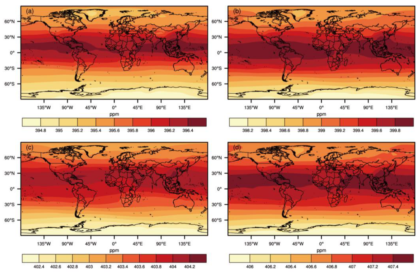
Using the fluxes of Scheme 2, the annual distribution of the global $\overline{{\mathrm{C}\mathrm{O}}_2}$ concentration from 2018 to 2021 could be obtained (Figure 6). The figure shows that the CO₂ concentrations in the middle- and low-latitude regions were higher than those in the high-latitude regions. Moreover, the CO₂ concentrations in the Northern Hemisphere were greater than those in the Southern Hemisphere. These results intuitively reflected the characteristics of the nonuniform distribution of the global CO₂ concentration. In addition, the global CO₂ concentrations were increasing annually, which was consistent with GAW’s observation results. The simulated surface CO₂ concentrations in China exhibited a pattern of seasonal variation, with a low concentration in summer and a high concentration in winter (Figure 7). In summer, due to vigorous vegetation growth and intense photosynthesis [43], the surface CO₂ concentrations were low. In winter, due to the respiration of plants and soil, and the release of vegetation into the atmosphere in the form of CO₂ after decay, resulting in high surface CO₂ concentrations [44,45]. In addition to noticeable seasonal changes, the surface CO₂ concentrations in China have also shown a clear increasing trend annually, which is caused by the accumulation of anthropogenic emissions.

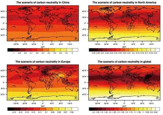
3.3. The Scenario of Carbon Neutrality in China

Before discussing the impact of carbon neutrality on CO₂ concentration, we added Scheme 7 to demonstrate the rationality of the method we used. Firstly, the optimized flux-driven atmospheric transport model were used to obtain the global distribution of CO₂ concentration (Scheme 2). Then, after removing China’s fluxes, the atmospheric transport model was run to obtain the distribution of global CO₂ concentration after China reached carbon neutrality (Scheme 3). The difference between the above two results was the impact of China’s carbon neutrality on global CO₂ concentration. Removing the flux from China to operate the model may result in concentration gradients, so we ran the case of only retaining the fluxes from China to test whether concentration gradients would occur (Scheme 7). Firstly, we subtracted the results of Scheme 6 from the results of Schemes 2, 3, and 7 to avoid the influence of the background field on the results. Then, we added the results of Scheme 3 and Scheme 7, and compared the added results with Scheme 2, as shown in Figure 8. After removing the flux from a certain region, there were no concentration gradients; thus, our method was reasonable.

Subtracting the $\overline{{\mathrm{C}\mathrm{O}}_2}$ values obtained from Scheme 2 and Scheme 3 revealed the changes in global CO₂ concentrations after China achieved net zero anthropogenic CO₂ emissions, as shown in Figure 9a. After removing the fluxes from China, the CO₂ concentrations in all world regions decreased. The CO₂ concentrations in China decreased the most, especially in the eastern region of China, followed by other areas in the Northern Hemisphere at the same latitude as that in China. In contrast, the CO₂ concentrations in the Southern Hemisphere decreased relatively less. Realizing carbon neutrality can bring benefits in mitigating global climate change, controlling air pollution, human health [46], and protecting biodiversity [47]. Quantitative analysis of the impact of achieving carbon neutrality in a specific region on global CO₂ concentration can help us gain a deeper understanding of this benefit. After removing the Chinese flux, the global CO₂ concentration decreased by 0.58 ppm, the CO₂ concentration in China decreased by 0.71 ppm, and the CO₂ concentration decreased by 0.66 ppm and 0.65 ppm in North America and Europe. These results indicated that China’s terrestrial ecosystem, ocean, fossil fuel, and fire flux all contribute to global CO₂ concentrations, with the factors mentioned making the largest contributions to China’s CO₂ concentrations. Although there are still some uncertainties in the estimation of carbon sinks in China’s terrestrial ecosystems, most studies [21,22,24] have shown that China’s terrestrial ecosystems are a carbon sink; have also conducted relevant research in the early stage [48]. In addition, the use of fire flux as a carbon source is relatively small in China. Therefore, the dominant factor causing this phenomenon is the decrease in fossil fuel flux after carbon neutrality, and the emission source will directly impact the local CO₂ concentrations. Figure 9b shows that the average wind direction at 100 m in the mid-latitudes of the Northern Hemisphere from 2018 to 2021 was west. Therefore, due to the transportation effect of meteorology, the fluxes emitted by China under the influence of westerly winds will also impact the CO₂ concentrations in regions at the same latitude as China in the Northern Hemisphere.

Figure 9c shows the distribution of the $\overline{{\mathrm{C}\mathrm{O}}_2}$ difference between Scheme 2 and Scheme 3 in China. After removing the fluxes from China, the CO₂ concentrations in the eastern regions of China decreased the most, especially in North China, Central China, and East China, which are also areas with relatively high fossil fuel emissions (as shown in Figure 9d). Figure 9e,f shows the distributions of the $\overline{{\mathrm{C}\mathrm{O}}_2}$ differences between Scheme 2 and Scheme 3 in North America and Europe after removing the fluxes from China. The figures show that after removing the fluxes from China, the CO₂ concentrations in the southern United States, Mexico, and southern Europe decreased the most because these regions are at the same latitude as China. Therefore, under the influence of the westerly winds in the Northern Hemisphere, these regions are more affected than others.

Then, we studied the contribution rates of China’s fluxes to the annual $\overline{{\mathrm{C}\mathrm{O}}_2}$ concentration growth in China, North America, and Europe. To eliminate the influence of meteorological fields on concentrations, we set Scheme 6 and obtained the concentration field output of the TM5 model without prior flux input. We took the contribution rate of China’s fluxes to the annual $\overline{{\mathrm{C}\mathrm{O}}_2}$ concentration growth in China as an example, and other situations could be obtained using the same calculation method. First, we calculated the annual average $\overline{{\mathrm{C}\mathrm{O}}_2}$ concentrations in China under Schemes 2, 3, and 6. To eliminate the influence of meteorological fields, the annual average concentrations obtained from Schemes 2 and 3 were subtracted from the average concentrations obtained from Scheme 6. To calculate the concentration growth, we subtracted the concentrations from the previous year from the concentrations of the following year. Finally, we divided the results from Scheme 3 by Scheme 2 to obtain the contribution rate of fluxes from other regions to the annual average concentration growth in China after removing the flux from China. The remaining factor was the contribution rate of fluxes from China to the yearly average concentration growth in China. Through this calculation method, it could be concluded that the average contribution rates of China’s fluxes to the annual $\overline{{\mathrm{C}\mathrm{O}}_2}$ concentration growth in China, North America, and Europe were approximately 46.96%, 46.93%, and 46.89%, respectively. This significant contribution may be related to China’s high fossil fuel emissions.

The annual variation of surface CO₂ concentrations obtained from Scheme 2 and Scheme 3, as shown in Figure 10, revealed that after China reached carbon neutrality, the global average surface CO₂ concentrations decreased annually, with the least decrease occurring in 2018 and the greatest decrease occurring in 2021. This may be because the CO₂ concentrations in the atmosphere is a long-term accumulation result; that is, after carbon fluxes are emitted into the atmosphere, the impact on CO₂ concentrations in the atmosphere has a lag period. Therefore, as time progresses, the impact of emission fluxes on concentrations gradually increases, leading to the most significant decrease occurring in 2021.

3.4. The Scenario of Carbon Neutrality in North America

Then, we analyzed how North American carbon neutrality would contribute to global CO₂ concentrations. Figure 11a shows the differences in $\overline{{\mathrm{C}\mathrm{O}}_2}$ obtained from Scheme 2 and Scheme 4. The figure shows that after removing the fluxes in North America, the global CO₂ concentrations decreased. The concentrations decreased the most in the United States, especially the southeastern United States, and for other regions at the same latitude as the United States, the concentrations also significantly reduced. This may be due to meteorological transport. The CO₂ concentrations in the Southern Hemisphere also decreased, but the magnitude of the decrease was substantially lower than that in the Northern Hemisphere. From the quantitative analysis, after removing the CO₂ fluxes in North America, the global CO₂ concentration decreased by 0.22 ppm, the CO₂ concentration in China decreased by 0.25 ppm, the CO₂ concentration in North America decreased by 0.23 ppm, and the CO₂ concentration in Europe decreased by 0.24 ppm.

Interestingly, as the two largest countries in North America, the impact of North American fluxes on CO₂ concentrations in the United States was significantly greater than that in Canada, with CO₂ concentrations in the United States decreasing by 0.25 ppm after removing the North American fluxes, while Canada’s CO₂ concentration decreased by only 0.22 ppm. We speculate that this may be because fossil fuel flux has an effect, and fossil fuel emissions in the United States are greater than those in Canada. According to the GCP [28], from 2018 to 2021, fossil fuel emissions in the United States were approximately 1.39 Pg C/yr, while during the same period, Canadian fossil fuel emissions were much lower than those in the United States, with a value of 0.17 Pg C/yr. If North America reaches carbon neutrality, the United States needs to reduce more anthropogenic CO₂ emissions than other regions in North America; thus, the impact on CO₂ concentrations in the United States is more significant. From the above results, we can see that fossil fuel emissions are not proportional to the reduction in CO₂ concentration, because fossil fuel emissions are not the only factor affecting atmospheric CO₂ concentration.

There are differences between the results of Scheme 2 and 4 in North America, China, and Europe (Figure 11b–d). As shown in the figure, in high-value fossil fuel emission areas such as the eastern and southern United States and central Mexico (Figure 11c), after removing the fluxes, the impact on the CO₂ concentrations was significantly more significant than in other regions of North America. Like in China, under the influence of meteorological conditions, eliminating North American fluxes in Scheme 4 also greatly impacted northern China and southern Europe, which are at the same latitude as areas with high fossil fuel emission in North America.

Using the same method as in Scheme 3, the average contribution rates of North American fluxes to the annual $\overline{{\mathrm{C}\mathrm{O}}_2}$ concentration growth in China, North America, and Europe were calculated to be approximately 17.01%, 17.35%, and 17.25%, respectively.

3.5. The Scenario of Carbon Neutrality in Europe

Figure 12a shows the distribution of $\overline{{\mathrm{C}\mathrm{O}}_2}$ concentration differences between Scheme 2 and Scheme 5 after achieving carbon neutrality in Europe. It can be seen from the figure that after removing the fluxes in Europe, the greatest decrease in CO₂ concentration was seen in Europe, especially in western Europe, with other regions in the Northern Hemisphere also showing significant reductions. In terms of quantity, after removing the European fluxes, the global CO₂ concentration decreased by 0.10 ppm, the CO₂ concentration decreased by 0.10 ppm in China, the CO₂ concentration decreased by 0.12 ppm in North America, and the CO₂ concentration decreased by 0.12 ppm in Europe.

After removing European fluxes, differences in $\overline{{\mathrm{C}\mathrm{O}}_2}$ concentration remain between Scheme 2 and 5 in Europe, China, and North America. Figure 12c shows that western Europe’s fossil fuel flux emissions were greater. Therefore, after removing the European fluxes, the CO₂ concentrations in this region decreased most significantly. Under the influence of the westerly winds in the Northern Hemisphere, the impacts on northeastern China and the central United States were more significant than those on other regions. Interestingly, the decrease in CO₂ concentrations in China was significantly smaller than that in other regions of the Northern Hemisphere, especially in the Qinghai–Tibet Plateau region. This may be due to the high altitude of the Qinghai–Tibet Plateau, which is less affected by surface anthropogenic carbon emissions and hinders the impact of climate transfer downstream.

The results of the above three schemes showed that China’s carbon neutrality had the most significant impact on the global CO₂ concentrations, followed by North America and Europe, which was related to the fossil fuel emission values of the three countries and regions. According to the GCP [28], China’s fossil fuel emissions from 2018 to 2021 were approximately 2.9 Pg C/yr, North America’s fossil fuel emissions were about 1.53 Pg C/yr, and Europe’s fossil fuel emissions were about 1.31 Pg C/yr. Clearly, China needs to reduce the most anthropogenic CO₂ emissions in order to achieve the carbon neutrality goal, thereby reducing global CO₂ concentrations the most. However, the decrease in CO₂ concentration is not directly proportional to fossil fuel emissions, as meteorological transport also plays a certain role in it.

Then, we calculated the average contribution rates of the European flux to the annual $\overline{{\mathrm{C}\mathrm{O}}_2}$ concentration growth in China, North America, and Europe. Similar to the above calculation process, the results were approximately 8.20%, 8.48%, and 9.05%, respectively. The above three sets of contribution rate results indicated that the flux in a specific region significantly impacts the annual increase in CO₂ concentration in other regions, with the greatest impact on the local area. From 2018 to 2021, China’s fossil fuel emissions accounted for 29.4% of the total global fossil fuel emissions, North America’s fossil fuel emissions accounted for 15.5% of the total global fossil fuel emissions, and Europe’s fossil fuel emissions accounted for 13.3% of the total global fossil fuel emissions. The corresponding result was that China had the highest contribution rate to annual concentration growth in other regions, followed by North America and Europe. However, the proportion of emissions in each country and area does not correspond to the average contribution rate of annual concentration growth in that region, as the contribution rate of annual concentration growth is related not only to emissions but also to atmospheric transport.

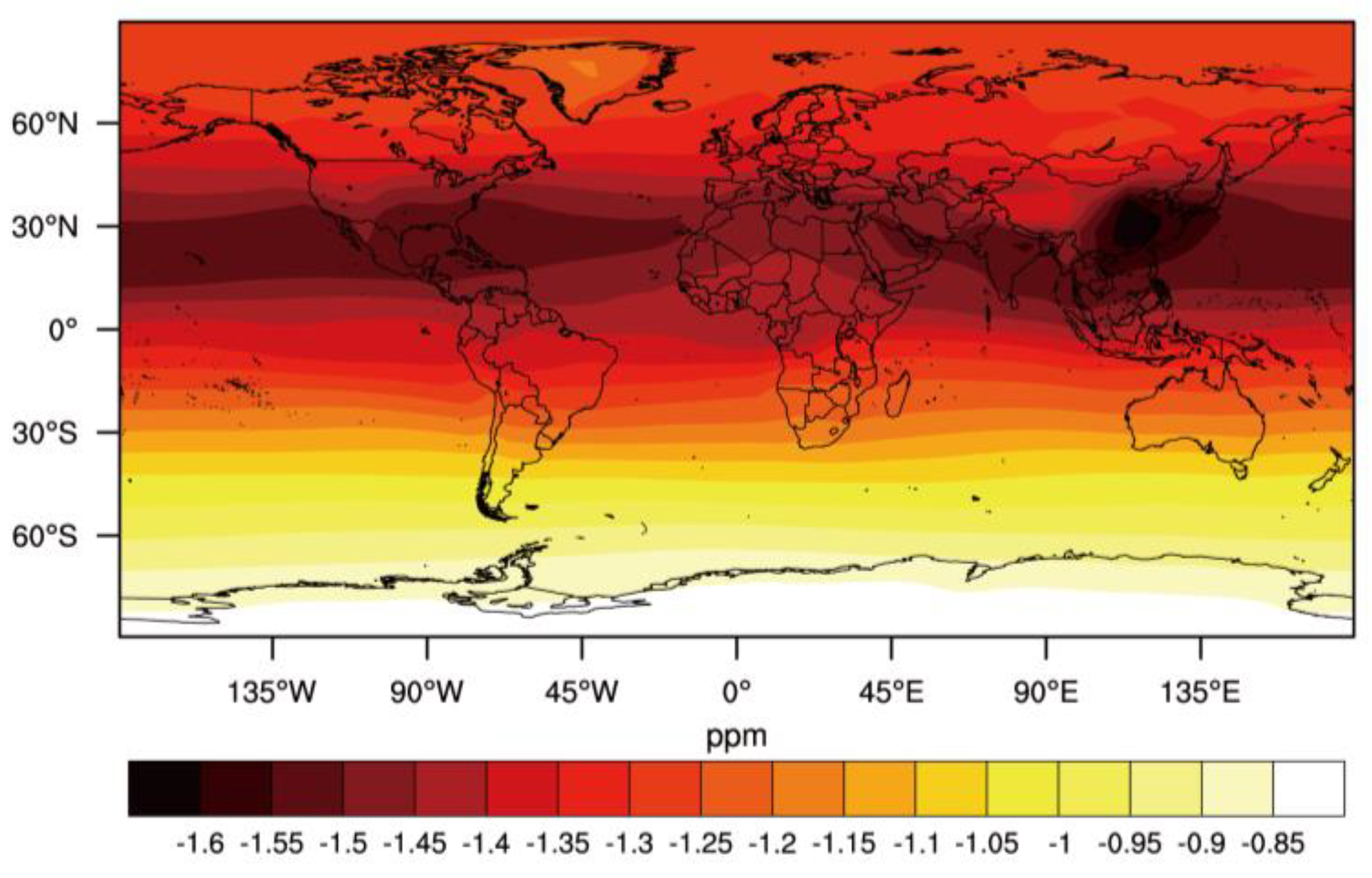
3.6. The Scenario of Carbon Neutrality in Global

Subtracting the $\overline{{\mathrm{C}\mathrm{O}}_2}$ values obtained from Scheme 2 and Scheme 6 revealed the changes in global CO₂ concentrations after the whole world achieves net zero anthropogenic CO₂ emissions, as shown in Figure 13. After reaching carbon neutrality globally, CO₂ concentrations would significantly decrease globally, especially in China, India, southern North America, and regions at the same latitude as them. This is because these countries and regions currently have relatively high total anthropogenic carbon emissions, and under the influence of westerly winds, they have a significant impact on other regions in the Northern Hemisphere. From a quantitative point of view, after global carbon neutrality, the global CO₂ concentration would decrease by 1.23 ppm, CO₂ concentration would decrease by 1.45 ppm in China, CO₂ concentration would decrease by 1.36 ppm in North America, and CO₂ concentration would decrease by 1.35 ppm in Europe.

Due to the direct impact of anthropogenic carbon emissions on surface CO₂ concentrations, we focused on the variation of surface CO₂ concentration with altitude in the following section. Figure 14 shows the daily variation of surface CO₂ concentration under the scenario of global carbon neutrality. After removing the global carbon fluxes, the average surface CO₂ concentrations significantly decreased and then stabilized at a value of approximately 405.9 ppm. Correspondingly, the high-level CO₂ concentration experienced a state of first increasing and then stabilizing, which was caused by vertical transport. Therefore, carbon neutrality has profound significance for controlling the whole layer of CO₂ concentrations in the atmosphere.

Similar to Figure 10, we compared the global surface average CO₂ concentrations of Scheme 2 and Scheme 6, and obtained Figure 15. Comparing the two figures, under the carbon neutrality scenario in China, the global surface CO₂ concentrations are still increasing, but the increase rate is slowing down. However, under the global carbon neutrality scenario, the global surface CO₂ concentrations are decreasing yearly. This phenomenon indicates that in order to mitigate global climate change, efforts from individual countries alone cannot be relied on, and global participation is needed. Each country should follow the principle of “common but differentiated responsibilities” proposed by the United Nations Framework Convention on Climate Change (UNFCCC) [49].

4. Conclusions and Discussion

Here, we used the prior and posterior data of terrestrial-marine aquatic ecosystems’ carbon exchange from the CCMVS-G system and anthropogenic carbon fluxes, mainly from fossil fuel and fire flux, driving the atmospheric chemical transport model TM5 to reveal the impact of uncertainty in input fluxes on model simulation results. The global CO₂ concentration distribution was simulated by more accurate input fluxes. By removing CO₂ fluxes from certain key regions, the impact of achieving carbon neutrality in these regions on CO₂ concentrations in other regions and globally was quantified. The conclusions of this study are as follows: 1. The results indicated that whether from the comparison of global surface CO₂ concentration with other product observations, or from the comparison of simulated and observed concentrations at CO₂ observation stations, the results obtained using posterior flux were more accurate and in line with actual situations. 2. The global CO₂ concentration exhibited a nonuniform spatial distribution, with CO₂ concentrations in mid to low latitudes higher than those in high latitudes, and that the relatively higher CO₂ concentration area extended toward the Northern Hemisphere. From 2018 to 2021, the global CO₂ concentration exhibited a temporal distribution pattern of increase yearly. Due to the influence of photosynthesis, China’s surface CO₂ concentrations showed seasonal variation characteristics, mainly manifested as a low concentration in summer and a high concentration in winter. 3. Assuming China, North America, and Europe achieve carbon neutrality, one can eliminate the anthropogenic carbon emissions in these areas. We can quantitatively analyze the impact of carbon neutrality on the CO₂ concentration in these regions and globally. After China reached carbon neutrality, the global CO₂ concentration decreased by 0.58 ppm, and the CO₂ concentration in China decreased by 0.71 ppm. After achieving carbon neutrality in North America, the global CO₂ concentration decreased by 0.22 ppm, and the CO₂ concentration in North America decreased by 0.23 ppm. After achieving carbon neutrality in Europe, the global CO₂ concentration decreased by 0.10 ppm, while the CO₂ concentration in Europe decreased by 0.12 ppm. Fossil fuel combustion remains the primary controlling factor for global atmospheric CO₂ concentration changes, and the anthropogenic emissions in the three regions mentioned above significantly impact global atmospheric CO₂ concentration. In areas where fluxes are removed, especially in areas with high fossil fuel emissions, the CO₂ concentrations decreased the most because the emission source has the most direct impact on the CO₂ concentrations above the local area, followed by other areas at the same latitude as these areas, which are mainly affected by the transportation of westerly winds in the Northern Hemisphere. Significantly reducing anthropogenic carbon emissions in critical regions worldwide is crucial for effectively lowering global atmospheric CO₂ concentrations and their impact on radiation balance. The relationship between coordinated development and emission reduction in the key areas is essential for achieving effective and timely reductions. 4. The global carbon neutrality scenario also tells us that in order to control CO₂ concentrations, we cannot rely solely on reducing emissions in a few key regions, but require joint efforts from all countries.

Our global CCMVS-G system is based on CGHGNET, a richer observation network that enables us to invert posterior terrestrial ecosystem and ocean fluxes with lower uncertainty. This helps us better use atmospheric chemical transport models to simulate global CO₂ concentration distribution and quantitatively analyze the impact of carbon neutrality on CO₂ concentration changes. In the past, few studies have used so many observation stations to operate the global carbon assimilation system. In the future, there are still some areas that can be improved. Firstly, the current CO₂ observation network in China is constantly improving, and in the future, using more Chinese CO₂ observation stations can effectively improve assimilation results. Secondly, considering the running time, the horizontal and vertical spatial resolution of the atmospheric chemical transport model we use can continue to be improved, and higher spatial resolution can be used in the future. Finally, this study only focuses on three countries and regions: China, North America, and Europe. In the future, it can focus on smaller regions, such as studying the impact of carbon neutrality in a province, which is of great significance for countries to specify emission reduction measures.