
SWOT Level 2 Lake Single-Pass Product: The L2_HR_LakeSP Data Preliminary Analysis for Water Level Monitoring

1
Department of Civil, Construction and Environmental Engineering (DICEA), Geodesy and Geomatics Division, Sapienza University of Rome, 00184 Rome, Italy
2
Sapienza School for Advanced Studies, Sapienza University of Rome, 00161 Rome, Italy
*
Author to whom correspondence should be addressed.
Remote Sens. 2024, 16(7), 1244; https://doi.org/10.3390/rs16071244
Submission received: 4 February 2024
/
Revised: 28 March 2024
/
Accepted: 30 March 2024
/
Published: 31 March 2024
(This article belongs to the Section Earth Observation Data)
Abstract
:The Surface Water and Ocean Topography (SWOT) mission, launched in December 2022, aims to address the crucial environmental goal of water monitoring to support preparedness for extreme events and facilitate adaptation to climate change on global and local scales. This mission will provide a comprehensive inventory of worldwide water resources, lakes, reservoir storage, and river dynamics. In this work, we carried out a preliminary assessment of SWOT’s Lake product Level 2 version 1.1, also known as “L2_HR_LakeSP”. The analysis was performed across six diverse lakes on three continents, revealing an average median bias of 0.08 m with respect to the considered reference, after suitable outlier removal. An overall precision of 0.22 m was found, combined with an average correlation of 68% between SWOT and reference time series. Moreover, the accuracy varied in the considered six lakes, since biases up to some decimeters were found for some of them; they could be due to residual inconsistencies between the vertical reference frame of SWOT and that of the considered reference. In summary, the first analysis of the “L2_HR_LakeSP” product, Version 1.1, demonstrated the promising potential of SWOT for monitoring seasonal variations in water levels. Nevertheless, notable anomalies were found in the water masks, particularly in higher latitudes, suggesting potential difficulties in accurately delineating water bodies in those regions. Additionally, a discernible reduction in accuracy was observed towards the end of the monitoring period. These preliminary findings indicate some issues that should be addressed in future investigations about the quality and potential of SWOT’s lake products for advancing our understanding of global water dynamics.
1. Introduction
Lakes are an integral component of the water cycle and play a vital role within Earth’s ecosystems, influencing various facets of daily life on our planet [1]. The noticeable effects of climate change on these essential water sources highlight the importance of addressing and adapting to challenges related to variations in weather patterns, rising temperatures, and shifts in precipitation that directly impact water availability and quality.
A continuous and large-scale monitoring of lakes and reservoirs is thus more necessary than ever. In this regard, the availability of new Earth observation (EO) methodologies and sensors offers valuable insights while concurrently reducing the monitoring costs and mitigating the need for expensive gauge station installations and their continuous maintenance, especially in remote locations [2]. Hence, EO technologies can contribute to a more efficient and cost-effective safeguard of these crucial water resources in various applications, including but not limited to, water level and extent [3,4].
In particular, many satellite altimetry missions have been used for inland water level monitoring, including both LiDAR (light detection and ranging) and RADAR (radio detection and ranging) missions. ICESat-2 (Ice, Cloud, and land Elevation Satellite-2) and GEDI (Global Ecosystem Dynamics Investigation) are LiDAR altimeters that have demonstrated successful applications in monitoring inland water bodies, encompassing lakes and wide rivers thanks to their small footprint size [5,6,7].
Sentinel-6 [8], Sentinel-3 [9], HY-2 [10], Jason-3 [11], and Saral [12] collectively constitute a set of SAR (synthetic aperture radar) and RADAR missions developed for the monitoring of inland water levels. These advanced EO satellites can provide precise measurements of water surface levels and extent, aiding in assessing water level dynamics in lakes, rivers, and other inland water bodies. Their data are frequently employed by specialized services such as DAHITI [13] and Hydroweb [14], enhancing the capacity to monitor and understand variations in water levels on both regional and global scales.
In December 2022, the Surface Water and Ocean Topography (SWOT) mission was launched, with the primary objective to provide the first worldwide inventory of water resources, including rivers, lakes, and reservoirs, to observe the fine details of the ocean surface topography, and to measure how terrestrial surface water bodies change over time [15,16,17]. The SWOT commissioning phase lasted several months, and only in December 2023 were real data collected in April 2023 during the calibration and validation (CalVal) phase released, including reprocessed global high rate (HR) hydrology products [18].
Nevertheless, to the best of our knowledge, only preliminary studies have been carried out on SWOT simulated data to understand the quality and potential results of the to-be-expected (at the time of the studies) sensor for monitoring water bodies’ level and extent.
In an early study conducted by Lee et al. [19] in 2010, SWOT observations were simulated by integrating data from lake gauges, satellite radar altimeter, and satellite imagery (Envisat 18 Hz data and TOPEX/Poseidon) across the Peace–Athabasca Delta (PAD) region in Northern Alaska, and Western Siberia regions. The primary aim of the simulation was to investigate the errors in the estimation of storage change from the variation in water surface extent and level. The findings revealed that lakes larger than 1 km2 had relative errors typically below 5%, whereas lakes with a size of 1 hectare registered relative errors around 20%, highlighting the influence of the lake size on the precision of storage change measurements.
Ten years later, Desrochers et al. [20] employed imagery captured by more recent EO sensors (Sentinel 1, 2, and 3, Landsat 8, RCM, and Jason-3) to retrieve water level and extent over the PAD region in Canada. These data were given as input to France’s Space Agency (CNES) Large-Scale SWOT Simulator, only to evaluate the consistency and close coherence between simulated data and the actual water surface level and area, confirming the results of Lee et al. [19] with more updated EO instruments. The authors also noticed that the seasonal growth of vegetation reduced the accuracy of retrieving water surface area in the simulation.
Finally, Grippa et al. [21] utilized SWOT-like synthetic data generated by the SWOT simulator from NASA-JPL, over Agoufou Lake in Mali, and retrieved water levels with an accuracy close to 4 cm.
None of the aforementioned studies analyzed real SWOT measurements. In this paper, we aim to carry out the first preliminary investigation on SWOT’s real data quality for lake water level monitoring. Thus, our analysis focuses on the first public release of the “SWOT Level 2 Lake Single-Pass Vector Data Product” (Section 2.1.1). Indeed, although this first release of SWOT products has known limitations and the release of products with improved quality is planned for January 2024 [18], it is crucial to start to understand SWOT’s data accuracy and limitations and to familiarize ourselves with the sensor and its performance in lake water level monitoring on a large scale.
2. Data
2.1. SWOT
The SWOT mission, led by NASA, in collaboration with CNES, employs the Ka-band Radar Interferometer (KaRIn) as its principal instrument. SWOT is indeed the first mission to adopt the wide-swath altimeter radar interferometry [22] with the aim to provide a highly accurate two-dimensional mapping of ocean surface topography and land surface water elevation [23] in the form of water masks.
Specifically, SWOT generates water masks with the precision to resolve features as narrow as 100 m in width for rivers and of 250 × 250 m for lakes and reservoirs [24]. Each mask is associated with water level elevations characterized by an expected accuracy and precision of 10 cm and an expected slope accuracy of 1.7 cm/1 km (when averaging over water areas larger than 1 km2) [24,25,26].
SWOT’s orbit extends from 78° S to 78° N, covering at least 86% of the globe in its three-year-long mission. SWOT revisits the same path all over the Earth every 21 days in 292 unique orbits. The water surface elevation (WSE) measured by SWOT is referenced to the Earth Gravitational Model (EGM2008) [27] and corrected for media delays (wet and dry troposphere, ionosphere) and tidal effects (solid tide, load tide, and pole tide) [23,28].
2.1.1. “L2_HR_LakeSP” Product
For this study, we used the “SWOT Level 2 Lake Single-Pass Vector Data Product, Version 1.1”, released in December 2023 [18] and downloaded from NASA’s Earth Data platform. The product, also known as “L2_HR_LakeSP”, is designed to provide lake-related measurements obtained within each continental pass from the HR data stream of the SWOT KaRIn instrument.
In particular, the L2_HR_LakeSP vector product is obtained from the KaRIn measured height, geolocation, and classification data available in the “Level 2 KaRIn high rate water mask pixel cloud product” (L2_HR_PIXC) [29]. The KaRIn instrument indeed employs cross-track interferometry to map the Earth-surface topography in 3D, producing the so-called “pixel cloud” (PIXC) [29]. PIXC represents the water mask for each considered water body, and it is organized as an unstructured list of geolocated interferogram pixels (latitude, longitude, and height), classified as water pixels (the majority) or land pixels (e.g., pixels in the pruning mask representing inclusion zones) [30]. The shape (in the form of a polygon) and the corresponding boundary of each water body, which constitute the L2_HR_LakeSP product, are retrieved by applying the concave hull algorithm to the water edge pixels of the PIXC, after the application of a height-constrained geolocation regularization [31]. Finally, several attributes, including average WSE, area, and derived storage change, are computed considering all the water pixels of the PIXC within the considered lake boundary and then associated with the corresponding polygon.
At the time of writing, the L2_HR_LakeSP product v.1.1 included just the lake polygons retrieved from the SWOT data collected in April 2023 (Figure 1). These data were captured during the one-day repeat cycle of the CalVal phase of SWOT [18,32], which occurred from April to July 2023. Thus, the dataset is characterized by a high temporal resolution, including at least one observation per day for each lake considered in this research.
The current L2_HR_LakeSP product release (v.1.1) comprises the water polygons in the form of shapefiles for lakes identified in the “prior lake database”, as well as newly detected features that were not present in the “prior river or lake databases” [23].
The data coverage extends across the entire swath, providing a comprehensive view of individual continents for each half orbit.
2.1.2. Available Attributes
The L2_HR_LakeSP product consists of 37 attributes including the WSE with respect to the geoid model EGM2008, calculated from an uncertainty-weighted average over all the water pixels of the PIXC (Section 2.1.1) within the bounds of the considered water body in the considered epoch.
It is important to note that for each considered water body, the lake boundary—and thus the polygon representing the lake shape—changes across different epochs (Figure 2) due to natural variations in the water body extension but also due to potential errors in SWOT measurements or SWOT processing algorithms.
In the L2_HR_LakeSP product, each fundamental observation (i.e., area, elevation) has an associated uncertainty. These uncertainties include errors from corrections, references, and random components. The product also includes the standard deviation of the WSE, computed over all the water pixels of the PIXC within the lake polygon, and the total estimated extension of the water surface and its uncertainties.
Other attributes are also available, including quality indicators (i.e., ice cover), geophysical references (i.e., geoid height and tides), geophysical range corrections (i.e., tropospheric path delay corrections), and instrument corrections.
2.2. Study Area, In Situ and Validation Data
Six different lakes with different characteristics were selected on three continents to assess the quality of the SWOT L2_HR_LakeSP product (Figure 1 and Table 1). In particular, for each lake, we compared the SWOT WSEs with the (as much as possible) contemporary reference water levels, gathered from different sources (Table 1).
For the lakes Ontario and Foss, we used the gauge measurements available from the National Oceanic and Atmospheric Administration (NOAA) and “US Army Corps of Engineers Tulsa District—Water Control Data System” networks as a reference.
For lakes Nasser and Balkhash, the reference data were obtained from the Hydroweb service, while for the Hirakud dam and the Bayano Lake, the reference data were requested from the DAHITI database, since Hydrospace data and the in situ measurements were unavailable. Notably, due to the scarce data availability from both DAHITI and Hydrospace services, a temporal linear interpolation was implemented to retrieve reference water level measurements corresponding to SWOT epochs for the four lakes for which gauge measurements were unavailable.
3. Method
Despite SWOT’s distinctive data-gathering procedure and complex processing algorithms, a substantial presence of outliers within the L2_HR_LakeSP product was observed. In this section, we describe the pre-processing steps and methodology implemented to effectively remove the outliers and enhance the quality of the resulting dataset.
3.1. Pre-Processing
The pre-processing of the L2_HR_LakeSP product involved the injection of this extensive dataset, available as ESRI shapefiles and exceeding 40 gigabytes, into a PostgreSQL database using PostGIS version 16.2 [33]. This migration was carried out to facilitate subsequent processing and enabled the implementation of spatial queries for the selection of the desired lakes, and the export of the selected data as analysis-ready tables. Moreover, the use of PostGIS allowed for an easy visualization of the data within QGIS.
3.2. Spatial Outlier Removal and Data Aggregation
The L2_HR_LakeSP product is organized in features: each lake can be represented as a continuous single feature, i.e., a polygon. However, in the case of larger lakes, it is common for a single lake to be represented by multiple features within one orbit, all sharing the same “Lake name” (Figure 3).
In other words, in the used release of the product, deriving from the one-day repeat cycle of the CalVal phase, for each lake, there was just one orbit, i.e., a passage of SWOT, per day, except for lakes located at the intersection of two orbits, like in the case of the Foss Lake (Figure 1 and Figure 4). In particular, for each SWOT passage over a lake, we can have several features in different temporally close epochs—a few seconds, or also in the very same epoch—with different shapes and extensions (Table 2), probably due to limitations in the current version of the water masking algorithm.
Hence, for each lake, we decided to temporally aggregate the data on the basis of the area covered by the features. Firstly, for every orbit belonging to each lake, we removed the measurements with an area lower than the 90th percentile of the total area of the measurements in the considered orbit. This step was applied to ensure that small polygons with different elevations did not affect the value of the temporally aggregated WSE.
Secondly, a daily weighted mean (wMean) based on the area was calculated to represent the WSE over the water body for each cycle of each pass. This step was necessary as larger features ensured lower random and systematic uncertainties, while smaller features included an extremely higher uncertainty and deviation from the average WSE, if compared to the reference (from gauge, DAHITI, or Hydroweb), highlighting a high number of outliers in SWOT data (Table 2).
Even though there was up to 2.5 m of difference between the remaining measurements in the same area (Table 2—the WSE of the features are marked with †), the daily area-weighted mean showed more resilience to the remaining outliers compared to the daily mean and daily median, as larger areas responded to a more accurate measurement (Table 2 and Figure 5).
3.3. Datum Transformation
The WGS84-EGM2008 height reference frame, the one employed by SWOT (Section 2.1), was chosen as the vertical height reference frame where to carry out the water level comparison and to which the reference water levels were transformed.
4. Results
To evaluate the accuracy of SWOT’s L2_HR_LakeSP data after the outlier removal, we conducted a comparative analysis for every considered lake by calculating the per-date differences between SWOT area-weighted mean WSEs and the corresponding reference measurements (Equation (1)), as well as standard statistics such as Pearson’s correlation coefficient:
where is the difference for the date i between the SWOT area-weighted mean WSE after the outlier removal (Section 3.2), denoted by , and the temporally closest reference water level measurement .
For each lake, the distribution of the differences across all the daily epochs was characterized through robust (median, NMAD and MAE) and nonrobust (mean difference, standard deviation and RMSE) statistics (Table 3).
Given the absence of reference data for all the daily SWOT epochs, we computed two overall statistics over all the lakes: the average and the reference-weighted average (the last two rows in Table 3). In the last case, the weights assigned to each lake were determined by the number of available reference observations. This method ensured a balanced and representative average, accounting for variations in the availability of reference information across different observation periods.
The results show that SWOT achieved the most accurate assessments of lake surface level variations in terms of the correlation coefficient (values equal to 0.89 and 0.71, respectively) for Lake Ontario and Lake Foss (Table 3), where actual gauge measurements were available as a reference. The lower SWOT performance in understanding variations in the remaining lakes may be attributed to potential biases in Hydrospace and DAHITI measurements, as well as limited reference data availability for some lakes (Table 3). Additionally, the temporal interpolation (Section 2.2) of reference data might miss capturing the actual variations in the water level, contributing to the observed underperformance in the lakes for which gauge measurements were unavailable. Moreover, the accuracy was variable, since biases up to some decimeters were evident for some lakes; they could be due to residual inconsistencies between the vertical reference frame of SWOT and that of the considered reference.
4.1. Accuracy Dependency on Time
Lake Foss, uniquely situated in Colorado at a point of intersection between two orbits (Figure 1), registered two measurements per day in the considered period, one at ≈4 a.m. (22:00 local time) and one at ≈4 p.m. (10:00 local time) (UTC). These measurements showed an intriguing pattern with variations up to 2 m between day and night, potentially linked to surface reflectance—which is impacted by factors such as sunlight angle and atmospheric conditions—and its effects on the sensor, overall resulting in a higher accuracy during the night time (Figure 4).
For Lake Balkhash, which recorded the lowest NMAD of 0.05 m and the highest accuracy with an RMSE of 0.06 m (Table 3), all the SWOT measurements were collected during the night time. Moreover, SWOT water level measurements for this lake were characterized by minimal variations overall, as shown by the weighted mean of the WSE in Figure 5 (a 0.01 m variation in the period under investigation).
4.2. Changes in Accuracy
One week after the start of the measurements, SWOT’s accuracy, here estimated as the difference between the SWOT area-weighted average WSE and the reference water levels, started to decrease. On the 21st and 22nd of April, an anomalous increase in the disagreement between the SWOT WSE and the reference water levels, up to 0.6 m in some cases, was also observable: this phenomenon might be due to the CalVal phase ongoing in the considered period or changes in the altitude of the platform hosting the KaRIn instrument (Figure 6).
4.3. Lake Polygons Distortions
Given the lack of previous studies about the L2_HR_LakeSP product, direct comparisons are impossible. Nevertheless, during the visual screening of the data, it came to our attention that SWOT lake polygons presented some distortions, particularly noticeable and more frequent at low and high latitudes (Figure 7). These anomalies may indicate challenges in accurately delineating water bodies in regions closer to the poles.
In consideration of the fact that one of SWOT’s mission objectives, in addition to water surface elevation monitoring, is the generation of area and volume change reports, the identified distortions in the data could potentially impact the accurate determination of water body area and volumes.
5. Conclusions
A preliminary accuracy and precision assessment of the SWOT Level 2 Lake Single-Pass Vector Data Product, Version 1.1, was carried out. After the removal of outliers, an average median difference of 0.08 m with respect to reference data was found over six different lakes on three continents. The overall precision of the data regarding the reference was equal to 0.22 m, with an overall correlation of 68%. Moreover, the accuracy was variable in the considered six lakes, since biases up to some decimeters were evident in some of them; they could be due to residual inconsistencies between the vertical reference frame of SWOT and that of the considered reference. Finally, understanding and addressing the drags in the lake polygons, and thus in the water masks, is crucial for ensuring the reliability and precision of SWOT measurements.
In summary, the first analysis of the SWOT Level 2 Lake Single-Pass Vector Data Product, Version 1.1, has demonstrated the promising potential of the KaRIn instrument for monitoring seasonal variations in water levels. Nevertheless, these preliminary findings indicate some issues that should be addressed in future investigations on the quality and potential of SWOT’s lake products for advancing our understanding of global inland water dynamics. Notably, as this investigation concerned the analysis of data collected during the CalVal phase, SWOT products are expected to achieve even higher precision in subsequent releases. As future developments, a more robust outlier removal procedure will be implemented, also analyzing the updated version of the lake products, in addition to understanding the effect of seiche, drags, gaps, and biases on the data quality over more lakes.
Author Contributions
Conceptualization, A.H., R.R. and M.C.; methodology, A.H.; software, A.H.; validation, A.H., R.R. and M.C.; formal analysis, A.H.; investigation, A.H.; resources, M.C.; data curation, A.H.; writing—original draft preparation, A.H.; writing—review and editing, A.H., R.R. and M.C.; visualization, A.H.; supervision, R.R. and M.C.; project administration, M.C.; funding acquisition, M.C. All authors have read and agreed to the published version of the manuscript.
Funding
A.H. was supported by the Doctoral Program fellowship within the program “PON Ricerca e Innovazione 2014–2020 Azioni IV.4 (DM1061)”, funded by Sapienza University of Rome. R.R. was supported by Sapienza University of Rome within the program “PON Ricerca e Innovazione 2014–2020 Azioni IV.4 (DM1062)”.
Data Availability Statement
The SWOT data is available on the Physical Oceanography Distributed Active Archive Center (PO.DAAC) of NASA-JPL (https://podaac.jpl.nasa.gov/SWOT?tab=mission-objectives§ions=about%2Bdata, accessed on 31 January 2024).
Conflicts of Interest
The authors declare no conflicts of interest.
References
- Sekertekin, A. A survey on global thresholding methods for mapping open water body using Sentinel-2 satellite imagery and normalized difference water index. Arch. Comput. Methods Eng. 2021, 28, 1335–1347. [Google Scholar] [CrossRef]
- Hamoudzadeh, A.; Ravanelli, R.; Crespi, M. GEDI data within Google Earth Engine: Potentials and analysis for inland surface water monitoring. In Proceedings of the EGU General Assembly 2023, Vienna, Austria, 23–28 April 2023. Technical Report. Copernicus Meetings. [Google Scholar] [CrossRef]
- Crétaux, J.F.; Abarca-del Río, R.; Berge-Nguyen, M.; Arsen, A.; Drolon, V.; Clos, G.; Maisongrande, P. Lake volume monitoring from space. Surv. Geophys. 2016, 37, 269–305. [Google Scholar] [CrossRef]
- Chang, N.B.; Imen, S.; Vannah, B. Remote sensing for monitoring surface water quality status and ecosystem state in relation to the nutrient cycle: A 40-year perspective. Crit. Rev. Environ. Sci. Technol. 2015, 45, 101–166. [Google Scholar] [CrossRef]
- Xu, N.; Zheng, H.; Ma, Y.; Yang, J.; Liu, X.; Wang, X. Global estimation and assessment of monthly lake/reservoir water level changes using ICESat-2 ATL13 products. Remote Sens. 2021, 13, 2744. [Google Scholar] [CrossRef]
- Fayad, I.; Baghdadi, N.; Bailly, J.S.; Frappart, F.; Zribi, M. Analysis of GEDI elevation data accuracy for inland waterbodies altimetry. Remote Sens. 2020, 12, 2714. [Google Scholar] [CrossRef]
- Hamoudzadeh, A.; Ravanelli, R.; Crespi, M. GEDI data withinGoogle Earth Engine: Preliminary analysis of a resource for inland surface water monitoring. Int. Arch. Photogramm. Remote Sens. Spat. Inf. Sci. 2023; XLVIII-M-1-2023, 131–136. [Google Scholar] [CrossRef]
- Donlon, C.J.; Cullen, R.; Giulicchi, L.; Vuilleumier, P.; Francis, C.R.; Kuschnerus, M.; Simpson, W.; Bouridah, A.; Caleno, M.; Bertoni, R.; et al. The Copernicus Sentinel-6 mission: Enhanced continuity of satellite sea level measurements from space. Remote Sens. Environ. 2021, 258, 112395. [Google Scholar] [CrossRef]
- Taburet, N.; Zawadzki, L.; Vayre, M.; Blumstein, D.; Le Gac, S.; Boy, F.; Raynal, M.; Labroue, S.; Crétaux, J.F.; Femenias, P. S3MPC: Improvement on inland water tracking and water level monitoring from the OLTC onboard Sentinel-3 altimeters. Remote Sens. 2020, 12, 3055. [Google Scholar] [CrossRef]
- Jiang, X.; Jia, Y.; Zhang, Y. Measurement analyses and evaluations of sea-level heights using the HY-2A satellite’s radar altimeter. Acta Oceanol. Sin. 2019, 38, 134–139. [Google Scholar] [CrossRef]
- Biancamaria, S.; Schaedele, T.; Blumstein, D.; Frappart, F.; Boy, F.; Desjonquères, J.D.; Pottier, C.; Blarel, F.; Niño, F. Validation of Jason-3 tracking modes over French rivers. Remote Sens. Environ. 2018, 209, 77–89. [Google Scholar] [CrossRef]
- Schwatke, C.; Dettmering, D.; Börgens, E.; Bosch, W. Potential of SARAL/AltiKa for inland water applications. Mar. Geod. 2015, 38, 626–643. [Google Scholar] [CrossRef]
- Schwatke, C.; Dettmering, D.; Bosch, W.; Seitz, F. DAHITI—An innovative approach for estimating water level time series over inland waters using multi-mission satellite altimetry. Hydrol. Earth Syst. Sci. 2015, 19, 4345–4364. [Google Scholar] [CrossRef]
- Laboratoire d’Etudes en Geophysique et Oceanographie, Equipe Geodesie, Oceanograhie et Hydrologie Spatiale). Hydroweb: Time Series of Water Levels in the Rivers and Lakes around the World. Available online: https://hydroweb.theia-land.fr (accessed on 31 January 2024).
- Riggs, R.M.; Allen, G.H.; Brinkerhoff, C.B.; Sikder, M.S.; Wang, J. Turning lakes into river gauges using the LakeFlow algorithm. Geophys. Res. Lett. 2023, 50, e2023GL103924. [Google Scholar] [CrossRef]
- Liu, K.; Song, C.; Zhao, S.; Wang, J.; Chen, T.; Zhan, P.; Fan, C.; Zhu, J. Mapping inundated bathymetry for estimating lake water storage changes from SRTM DEM: A global investigation. Remote Sens. Environ. 2024, 301, 113960. [Google Scholar] [CrossRef]
- Ma, C.; Guo, X.; Zhang, H.; Di, J.; Chen, G. An investigation of the influences of SWOT sampling and errors on ocean eddy observation. Remote Sens. 2020, 12, 2682. [Google Scholar] [CrossRef]
- SWOT JPL NASA Mission Team. SWOT Data: First Public Release. 2023. Available online: https://swot.jpl.nasa.gov/news/113/swot-data-first-public-release/ (accessed on 31 January 2024).
- Lee, H.; Durand, M.; Jung, H.C.; Alsdorf, D.; Shum, C.; Sheng, Y. Characterization of surface water storage changes in Arctic lakes using simulated SWOT measurements. Int. J. Remote Sens. 2010, 31, 3931–3953. [Google Scholar] [CrossRef]
- Desrochers, N.M.; Peters, D.L.; Siles, G.; Cauvier Charest, E.; Trudel, M.; Leconte, R. A Remote Sensing View of the 2020 Extreme Lake-Expansion Flood Event into the Peace–Athabasca Delta Floodplain—Implications for the Future SWOT Mission. Remote Sens. 2023, 15, 1278. [Google Scholar] [CrossRef]
- Grippa, M.; Rouzies, C.; Biancamaria, S.; Blumstein, D.; Cretaux, J.F.; Gal, L.; Robert, E.; Gosset, M.; Kergoat, L. Potential of SWOT for monitoring water volumes in Sahelian ponds and lakes. IEEE J. Sel. Top. Appl. Earth Obs. Remote Sens. 2019, 12, 2541–2549. [Google Scholar] [CrossRef]
- Rodriguez, E.; Fernandez, D.E.; Peral, E.; Chen, C.W.; De Bleser, J.W.; Williams, B. Wide-swath altimetry: A review. In Satellite Altimetry over Oceans and Land Surfaces; CRC Press: Boca Raton, FL, USA, 2017; pp. 71–112. [Google Scholar]
- CNES–JPL/NASA. Surface Water and Ocean Topography (SWOT) Project SWOT Product Description Long Name: Level 2 KaRIn High Rate Lake Single Pass Vector Product Short Name: L2_HR_LakeSP. 2023. Available online: https://podaac.jpl.nasa.gov/SWOT (accessed on 31 January 2024).
- SWOT. Archiving, Validation and Interpretation of Satellite Oceanographic Data (AVISO). 2024. Available online: www.aviso.altimetry.fr/en/missions/current-missions/swot.html (accessed on 31 January 2024).
- Fjørtoft, R.; Gaudin, J.M.; Pourthié, N.; Lalaurie, J.C.; Mallet, A.; Nouvel, J.F.; Martinot-Lagarde, J.; Oriot, H.; Borderies, P.; Ruiz, C.; et al. KaRIn on SWOT: Characteristics of near-nadir Ka-band interferometric SAR imagery. IEEE Trans. Geosci. Remote Sens. 2013, 52, 2172–2185. [Google Scholar] [CrossRef]
- Rodriguez, E.; Esteban-Fernandez, D. The Surface Water and Ocean Topography Mission (SWOT): The Ka-band Radar Interferometer (KaRIn) for water level measurements at all scales. In Proceedings of the Sensors, Systems, and Next-Generation Satellites XIV, Toulouse, France, 20–23 September 2010; Volume 7826, pp. 292–299. [Google Scholar]
- Pavlis, N.K.; Holmes, S.A.; Kenyon, S.C.; Factor, J.K. The development and evaluation of the Earth Gravitational Model 2008 (EGM2008). J. Geophys. Res. Solid Earth 2012, 117. [Google Scholar] [CrossRef]
- Wang, J.; Pottier, C.; Cazals, C.; Battude, M.; Sheng, Y.; Song, C.; Sikder, M.S.; Yang, X.; Ke, L.; Gosset, M.; et al. The Surface Water and Ocean Topography Mission (SWOT) Prior Lake Database (PLD): Lake mask and operational auxiliaries. ESS Open Arch. 2023, preprint. [Google Scholar]
- Williams, B.A.; Fjørtoft, R. Product Description Document—Level 2 KaRIn High Rate Water Mask Pixel Cloud Product (L2_HR_PIXC). JPL D-56411. 2023. [Google Scholar]
- Williams, B.; Fjørtoft, R. Pixel Cloud Product. 2017. Available online: https://swot.jpl.nasa.gov/system/documents/files/3761_3761_jun17_stm_37_williams.pdf (accessed on 31 January 2024).
- Pottier, C.; Stuurman, C. Algorithm Theoretical Basis Document Long Name: Level 2 KaRIn High Rate Lake Single Pass Science Algorithm Software: Level 2 Processing, Short Name: SAS_L2_HR_LakeSP: Level 2Processing. 2023. Available online: https://cmr.earthdata.nasa.gov/search/concepts/C2758162595-POCLOUD.html (accessed on 31 January 2024).
- Yaremchuk, M.; Beattie, C.; Panteleev, G.; D’Addezio, J.M.; Smith, S. The Effect of Spatially Correlated Errors on Sea Surface Height Retrieval from SWOT Altimetry. Remote Sens. 2023, 15, 4277. [Google Scholar] [CrossRef]
- Committee, P.P.S. PostGIS, Spatial and Geographic Objects for PostgreSQL. 2018. Available online: https://access.crunchydata.com/documentation/postgis/3.1.5/ (accessed on 31 January 2024).
- Rapp, R.H. Separation between reference surfaces of selected vertical datums. Bull. Géod. 1994, 69, 26–31. [Google Scholar] [CrossRef]
- National Oceanic and Atmospheric Administration. Online Vertical Datum Transformation. 2023. Available online: https://vdatum.noaa.gov/vdatumweb/ (accessed on 31 January 2024).
- Tapley, B.; Ries, J.; Bettadpur, S.; Chambers, D.; Cheng, M.; Condi, F.; Gunter, B.; Kang, Z.; Nagel, P.; Pastor, R.; et al. GGM02–An improved Earth gravity field model from GRACE. J. Geod. 2005, 79, 467–478. [Google Scholar] [CrossRef]
- Förste, C.; Bruinsma, S.; Abrikosov, O.; Lemoine, J.; Schaller, T.; Götze, H.; Ebbing, J.; Marty, J.; Flechtner, F.; Balmino, G.; et al. EIGEN-6C4. The Latest Combined Global Gravity Field Model Including GOCE Data up to Degree and Order 2190 of GFZ Potsdam and GRGS Toulouse. 2014, Volume 2190. Available online: https://dataservices.gfz-potsdam.de/icgem/showshort.php?id=escidoc:1119897 (accessed on 31 January 2024).
- Barthelmes, F. Definition of Functionals of the Geopotential and Their Calculation from Spherical Harmonic Models: Theory and Formulas Used by the Calculation Service of the International Centre for Global Earth Models (ICGEM). 2009. Available online: http://icgem.gfz-potsdam.de (accessed on 31 January 2024).
Figure 1.
Area covered by SWOT during the CalVal phase in April 2023 (black stripes) and the six lakes considered in this study (red dots).
Figure 1.
Area covered by SWOT during the CalVal phase in April 2023 (black stripes) and the six lakes considered in this study (red dots).
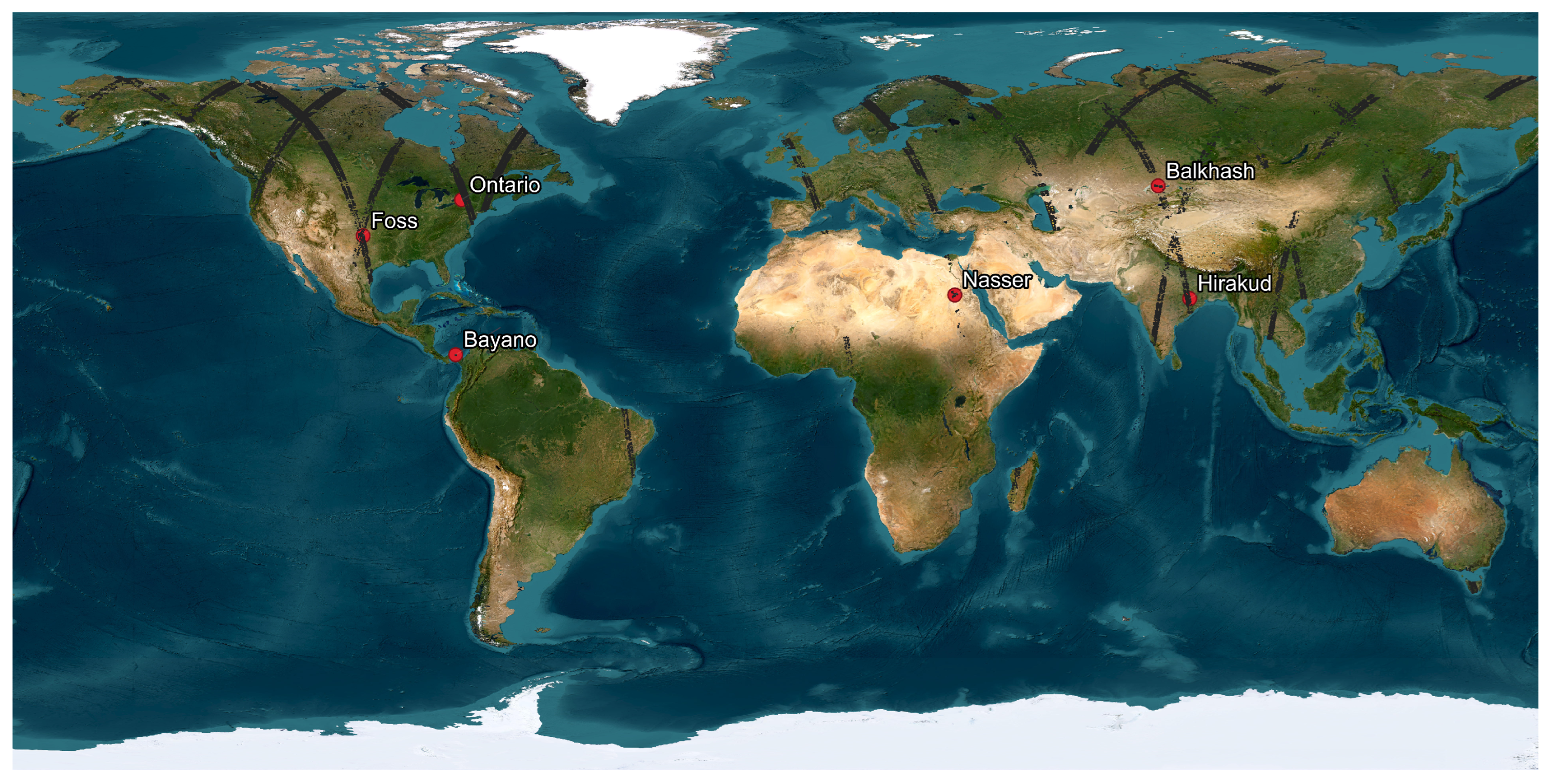
Figure 2.
Lake Foss: different boundary extents in the 36 different acquisitions of SWOT—each color represents a per epoch polygon (from 8 April 2023 to 26 April 2023).
Figure 2.
Lake Foss: different boundary extents in the 36 different acquisitions of SWOT—each color represents a per epoch polygon (from 8 April 2023 to 26 April 2023).
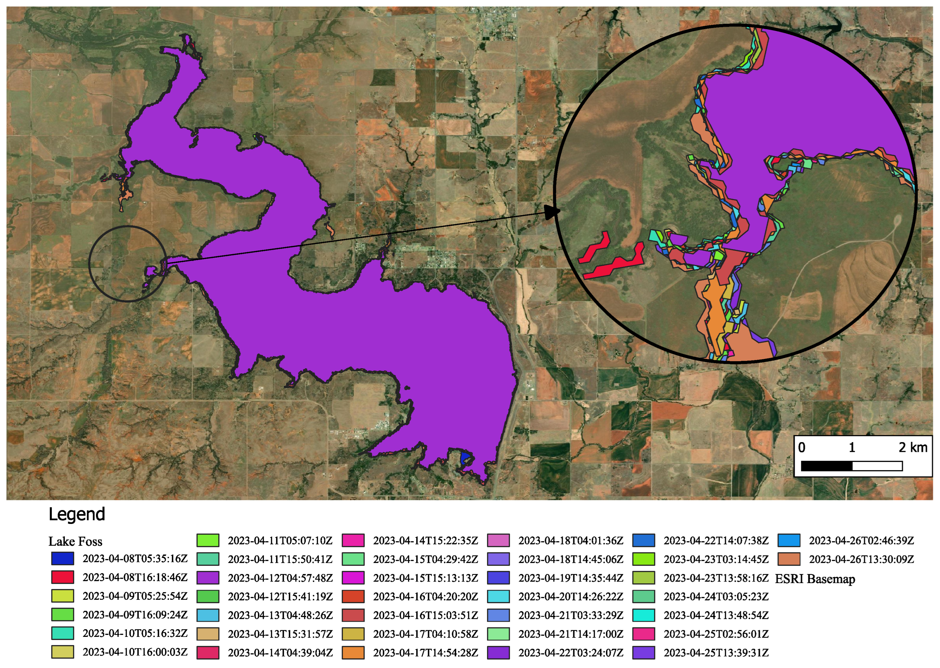
Figure 3.
Lake Ontario (North America): structure of multiple features over the same water body over a single orbit—each color represents a different feature.
Figure 3.
Lake Ontario (North America): structure of multiple features over the same water body over a single orbit—each color represents a different feature.
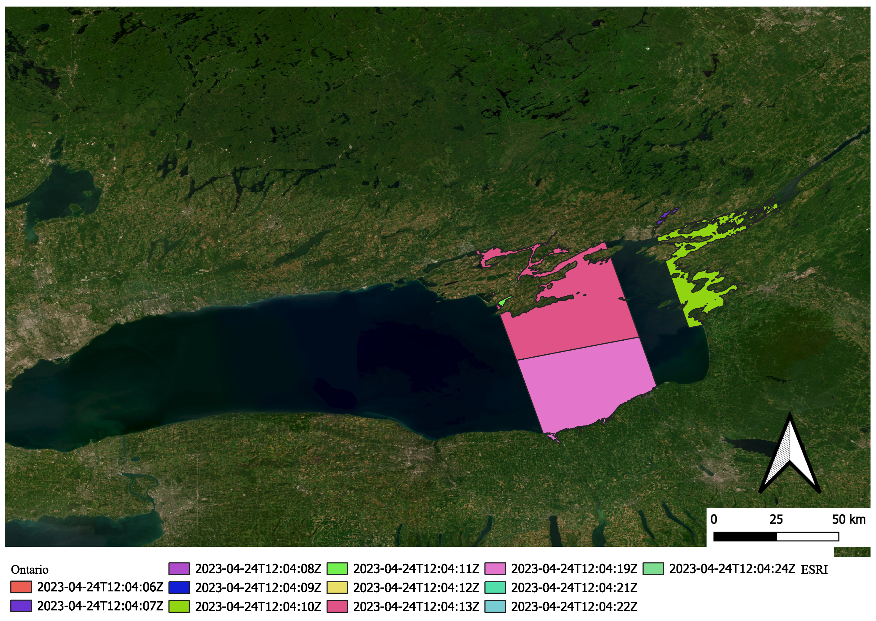
Figure 4.
Lake Foss: extreme variations through the day and night with the correspondent gauge measurement.
Figure 4.
Lake Foss: extreme variations through the day and night with the correspondent gauge measurement.
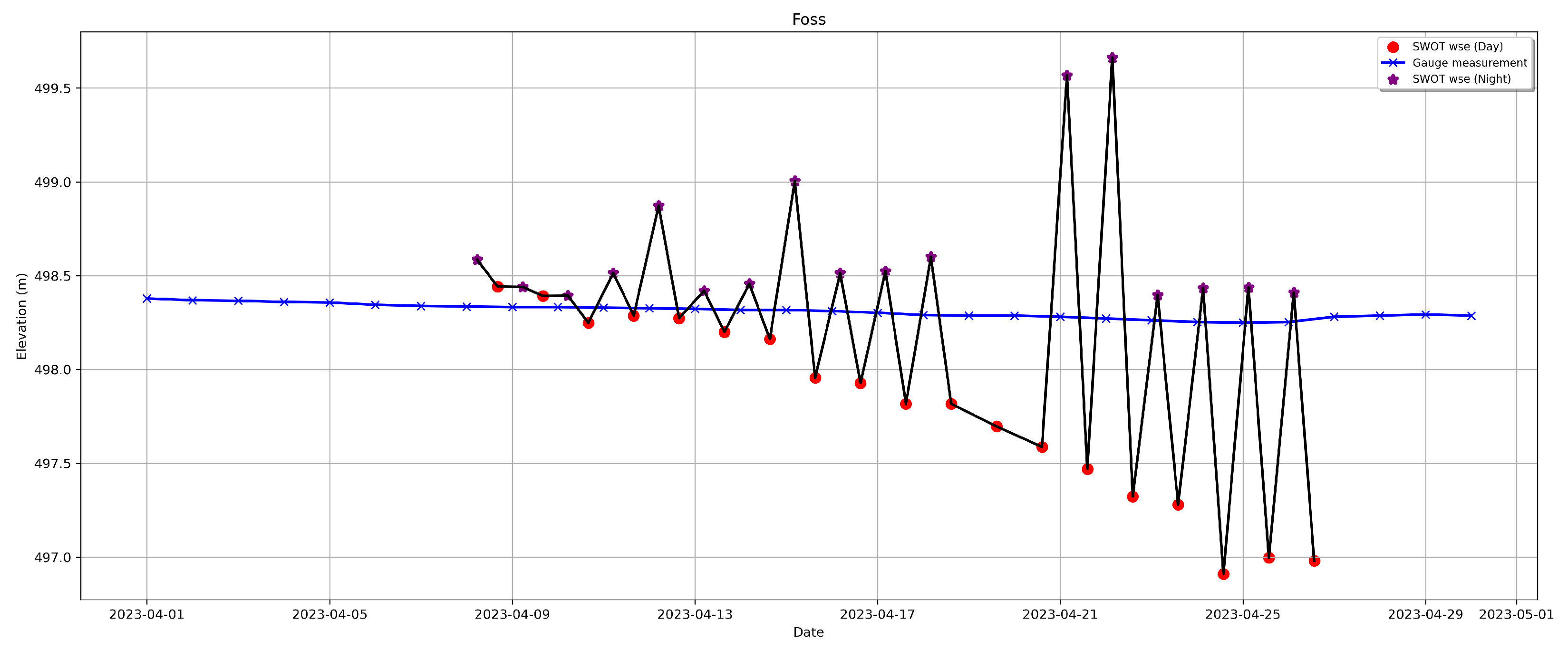
Figure 5.
Lake Balkhash: mean, area-weighted mean, and median SWOT WSE in comparison to Hydrospace (interpolated) reference data and the resilience of the area-weighted mean (wMean) to the high variation.
Figure 5.
Lake Balkhash: mean, area-weighted mean, and median SWOT WSE in comparison to Hydrospace (interpolated) reference data and the resilience of the area-weighted mean (wMean) to the high variation.

Figure 6.
The difference between the area-weighted average WSE and the corresponding reference for each cycle, anomalous increase in error on the 21st and 22nd of April, and the noticeable loss of accuracy after one week through all investigated lakes.
Figure 6.
The difference between the area-weighted average WSE and the corresponding reference for each cycle, anomalous increase in error on the 21st and 22nd of April, and the noticeable loss of accuracy after one week through all investigated lakes.
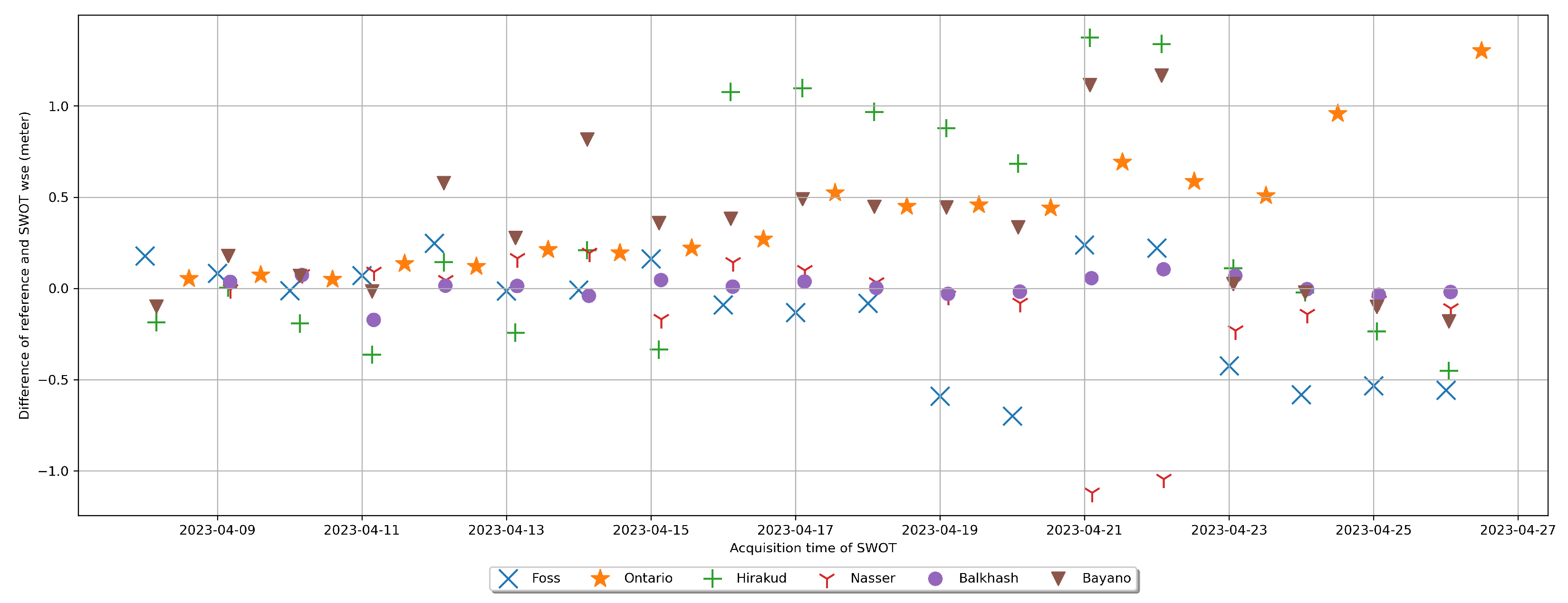
Figure 7.
Drags and distortion of features in Sweden: each color represents a different feature (lake).
Figure 7.
Drags and distortion of features in Sweden: each color represents a different feature (lake).


Table 1.
Investigated lakes, area, source of data used for validation and number or type of available observation.
Table 1.
Investigated lakes, area, source of data used for validation and number or type of available observation.
| Name | Center | Area (km2) | Reference |
|---|---|---|---|
| Ontario (North America) | 43°51′N 77°57′W | ≈19,000 | Gauge measurements |
| Foss (North America) | 35°33′N 99°13′W | ≈35 | Gauge measurements |
| Nasser (Egypt) | 22°30′N 31°52′E | ≈5250 | Hydrospace |
| Balkash (Kazakhstan) | 46°32′N 74° 52′E | ≈17,000 | Hydrospace |
| Hirakud dam (India) | 21°32′N 83°52′E | ≈740 | DAHITI |
| Bayano (Panama) | 9°09′N 78°46′W | ≈350 | DAHITI |
Table 2.
Water surface elevation and its uncertainties of all measurements of the same orbit of SWOT over the same water body (same as Figure 3)—Lake Ontario. * PassID represents the recurring pass (orbit) and cycleID represents the number of cycles over the same pass. † Remaining measurements after the use of the 90th percentile (Section 3.2). ‡ Statistics including area-weighted mean, mean, and median for the remaining features after the outlier removal (Section 3.2).
| time_str | cycleID_passID * | wse | wse_u | wse_r_u | wse_std | area_total |
|---|---|---|---|---|---|---|
| (UTC) | (m) | (m) | (m) | (m) | (km2) | |
| 24 April 2023 12:04:06 | 500_022 | 76.917 | 0.380 | 0.050 | 0.224 | 0.042573 |
| 24 April 2023 12:04:06 | 500_022 | 76.738 | 0.045 | 0.044 | 0.213 | 0.074521 |
| 24 April 2023 12:04:07 | 500_022 | 87.635 | 0.003 | 0.002 | 0.153 | 16.72101 |
| 24 April 2023 12:04:07 | 500_022 | 57.688 | 0.046 | 0.045 | 0.230 | 0.117021 |
| 24 April 2023 12:04:07 | 500_022 | 76.948 | 0.025 | 0.022 | 0.162 | 0.190093 |
| 24 April 2023 12:04:07 | 500_022 | 89.247 | 0.077 | 0.083 | 0.281 | 0.033036 |
| 24 April 2023 12:04:07 | 500_022 | 72.528 | 0.053 | 0.052 | 0.275 | 0.077082 |
| 24 April 2023 12:04:07 | 500_022 | 73.159 | 0.034 | 0.027 | 0.228 | 0.096808 |
| 24 April 2023 12:04:08 | 500_022 | 90.784 | 0.019 | 0.011 | 0.135 | 0.330947 |
| 24 April 2023 12:04:08 | 500_022 | 73.975 | 0.049 | 0.041 | 0.180 | 0.066079 |
| 24 April 2023 12:04:08 | 500_022 | 92.117 | 0.045 | 0.045 | 0.107 | 0.049441 |
| 24 April 2023 12:04:09 | 500_022 | 55.703 | 0.061 | 0.040 | 0.289 | 0.089956 |
| † 24 April 2023 12:04:10 | 500_022 | 73.826 | 0.001 | 0.000 | 0.495 | 723.1566 |
| 24 April 2023 12:04:11 | 500_022 | 77.038 | 0.004 | 0.003 | 0.264 | 11.26923 |
| 24 April 2023 12:04:12 | 500_022 | 83.056 | 0.051 | 0.029 | 0.099 | 0.067581 |
| 24 April 2023 12:04:12 | 500_022 | 79.763 | 0.059 | 0.061 | 0.222 | 0.049831 |
| † 24 April 2023 12:04:13 | 500_022 | 75.952 | 0.001 | 0.000 | 0.605 | 1985.917 |
| † 24 April 2023 12:04:19 | 500_022 | 76.088 | 0.001 | 0.000 | 0.535 | 1883.691 |
| 24 April 2023 12:04:21 | 500_022 | 85.217 | 0.258 | 0.039 | 0.480 | 0.036153 |
| 24 April 2023 12:04:22 | 500_022 | 93.767 | 0.238 | 0.024 | 0.276 | 0.488478 |
| 24 April 2023 12:04:24 | 500_022 | 76.930 | 0.095 | 0.083 | 0.299 | 0.029528 |
| ‡ Weighted mean | 75.67 | |||||
| ‡ Mean | 75.29 | |||||
| ‡ Median | 75.95 |
Table 3.
Standard statistics (mean difference (MD), median, standard deviation (SD), normalized median absolute deviation (NMAD), root-mean-square error (RMSE), mean absolute error (MAE), Pearson’s correlation coefficient) of the differences between the most synchronized water levels as derived from SWOT and reference data (for DAHITI and Hydrospace after the interpolation), the number of orbits and features within the dataset, and a reference-weighted statistics based on the number of actual reference data available, given as weights.
| Lake | MD | Median | SD | NMAD | RMSE | MAE | Correlation | Orbits | Total Features | Weights |
|---|---|---|---|---|---|---|---|---|---|---|
| (m) | (m) | (m) | (m) | (m) | (m) | (-) | (-) | (-) | (-) | |
| Ontario | 0.40 | 0.36 | 0.33 | 0.29 | 0.52 | 0.40 | 0.89 | 18 | 365 | 18 |
| Foss | −0.13 | −0.01 | 0.32 | 0.28 | 0.34 | 0.26 | 0.71 | 36 | 36 | 18 |
| Balkhash | 0.01 | 0.01 | 0.06 | 0.05 | 0.06 | 0.04 | 0.44 | 18 | 1735 | 10 |
| Hirakud | −0.12 | −0.02 | 0.37 | 0.17 | 0.38 | 0.21 | 0.71 | 18 | 233 | 2 |
| Nasser | −0.27 | −0.23 | 0.15 | 0.09 | 0.31 | 0.27 | 0.35 | 18 | 115 | 7 |
| Bayano | 0.33 | 0.34 | 0.39 | 0.40 | 0.50 | 0.37 | 0.78 | 19 | 122 | 2 |
| Average | 0.04 | 0.08 | 0.27 | 0.21 | 0.35 | 0.26 | 0.65 | - | 434 | - |
| wAverage | 0.06 | 0.10 | 0.26 | 0.22 | 0.35 | 0.27 | 0.68 | - | - | - |
Disclaimer/Publisher’s Note: The statements, opinions and data contained in all publications are solely those of the individual author(s) and contributor(s) and not of MDPI and/or the editor(s). MDPI and/or the editor(s) disclaim responsibility for any injury to people or property resulting from any ideas, methods, instructions or products referred to in the content. |
© 2024 by the authors. Licensee MDPI, Basel, Switzerland. This article is an open access article distributed under the terms and conditions of the Creative Commons Attribution (CC BY) license (https://creativecommons.org/licenses/by/4.0/).
Share and Cite
MDPI and ACS Style
Hamoudzadeh, A.; Ravanelli, R.; Crespi, M. SWOT Level 2 Lake Single-Pass Product: The L2_HR_LakeSP Data Preliminary Analysis for Water Level Monitoring. Remote Sens. 2024, 16, 1244. https://doi.org/10.3390/rs16071244
AMA Style
Hamoudzadeh A, Ravanelli R, Crespi M. SWOT Level 2 Lake Single-Pass Product: The L2_HR_LakeSP Data Preliminary Analysis for Water Level Monitoring. Remote Sensing. 2024; 16(7):1244. https://doi.org/10.3390/rs16071244
Chicago/Turabian StyleHamoudzadeh, Alireza, Roberta Ravanelli, and Mattia Crespi. 2024. "SWOT Level 2 Lake Single-Pass Product: The L2_HR_LakeSP Data Preliminary Analysis for Water Level Monitoring" Remote Sensing 16, no. 7: 1244. https://doi.org/10.3390/rs16071244
Note that from the first issue of 2016, this journal uses article numbers instead of page numbers. See further details here.