UAS Quality Control and Crop Three-Dimensional Characterization Framework Using Multi-Temporal LiDAR Data

Abstract

Information on a crop’s three-dimensional (3D) structure is important for plant phenotyping and precision agriculture (PA). Currently, light detection and ranging (LiDAR) has been proven to be the most effective tool for crop 3D characterization in constrained, e.g., indoor environments, using terrestrial laser scanners (TLSs). In recent years, affordable laser scanners onboard unmanned aerial systems (UASs) have been available for commercial applications. UAS laser scanners (ULSs) have recently been introduced, and their operational procedures are not well investigated particularly in an agricultural context for multi-temporal point clouds. To acquire seamless quality point clouds, ULS operational parameter assessment, e.g., flight altitude, pulse repetition rate (PRR), and the number of return laser echoes, becomes a non-trivial concern. This article therefore aims to investigate DJI Zenmuse L1 operational practices in an agricultural context using traditional point density, and multi-temporal canopy height modeling (CHM) techniques, in comparison with more advanced simulated full waveform (WF) analysis. Several pre-designed ULS flights were conducted over an experimental research site in Fargo, North Dakota, USA, on three dates. The flight altitudes varied from 50 m to 60 m above ground level (AGL) along with scanning modes, e.g., repetitive/non-repetitive, frequency modes 160/250 kHz, return echo modes (1n), (2n), and (3n), were assessed over diverse crop environments, e.g., dry corn, green corn, sunflower, soybean, and sugar beet, near to harvest yet with changing phenological stages. Our results showed that the return echo mode (2n) captures the canopy height better than the (1n) and (3n) modes, whereas (1n) provides the highest canopy penetration at 250 kHz compared with 160 kHz. Overall, the multi-temporal CHM heights were well correlated with the in situ height measurements with an R² (0.99–1.00) and root mean square error (RMSE) of (0.04–0.09) m. Among all the crops, the multi-temporal CHM of the soybeans showed the lowest height correlation with the R² (0.59–0.75) and RMSE (0.05–0.07) m. We showed that the weaker height correlation for the soybeans occurred due to the selective height underestimation of short crops influenced by crop phonologies. The results explained that the return echo mode, PRR, flight altitude, and multi-temporal CHM analysis were unable to completely decipher the ULS operational practices and phenological impact on acquired point clouds. For the first time in an agricultural context, we investigated and showed that crop phenology has a meaningful impact on acquired multi-temporal ULS point clouds compared with ULS operational practices revealed by WF analyses. Nonetheless, the present study established a state-of-the-art benchmark framework for ULS operational parameter optimization and 3D crop characterization using ULS multi-temporal simulated WF datasets.

1. Introduction

In precision agriculture (PA), imaging sensors have been extensively used across various platforms, e.g., satellites, aircraft, and manned/unmanned ground vehicles (UGVs), in outdoor and indoor settings [1,2,3,4]. In remote sensing, ground-based indoor/outdoor environments utilize what is known as proximal remote sensing (PRS), while aerial and space-borne sensor applications are usually categorized under remote sensing (RS) platforms [5]. PRS typically offers continuous data in restrained locations, concentrating on individual plants or groups situated in controlled environments [6]. On the other hand, RS platforms are primarily utilized in open environments for mapping extensive plant communities across wide areas comprising multiple agricultural experimental plots on the regional, state-wide, or even national scales [2]. To date, space-borne and aerial RS platforms in conjunction with PRS have enabled scientists and agronomists to study crop characteristics in a wide area capacity. RS ensures mapping and monitoring in a wide area capacity, whereas PRS by and large provides an evaluation counterpart or ground truth to assess the several complex plant traits and responses [6]. Indoor/outdoor PRS encounters various constraints, such as confinement to small areas, deployment challenges in inaccessible regions, and the need for labor-intensive human monitoring to keep sensor and controlled environments operational [5].

Recently, the advent of commercial unmanned aerial systems (UASs) has bridged the gap in wide-area mapping [7,8]. UASs, equipped with state-of-the-art sensors, address the limitations of PRS by providing very high-resolution (VHR) spatio-temporal resolutions [5,9]. Currently, UASs are capable of carrying various payloads for mapping and monitoring the biophysical and geochemical traits of plants with unparalleled spectral, spatial, and temporal resolutions, allowing for extensive area coverage [7,10]. For the past several decades, multispectral and hyperspectral imaging has been instrumental in PA research and development (R & D), mapping, and monitoring crop response to, e.g., climate change [11,12,13]. Among various phenological and geochemical traits, the geometric attributes of plants, such as height, size, crown area, stem size, leaf area, and leaf orientation, are crucial for investigating crop geometric-dependent functional traits [14,15,16]. Crops’ 3D characterization using PRS/RS is essential for responding to scientific inputs and climate change scenarios, thereby supporting (R & D) in phenotyping [5,17]. Traditionally, field-based manual plant geometric attribute measurements have been considered reliable, yet they are limited by being time consuming, labor intensive, intrusive, and subject to human errors [15,18,19]. Therefore, the 3D characterization of a crop’s geometric attributes in both indoor and outdoor settings has become essential [11].

Photogrammetry-based 3D modeling, VHR multispectral stereo-imagery acquired from ground-based indoor/outdoor settings or aerial platforms like UASs, has provided substantial assistance in PA and phenotyping [4,11,13]. Leveraging the principles of stereo-vision and structure from motion (SfM), photogrammetric techniques facilitate the extraction of the 3D morphology of plants, resulting in detailed 3D colored and textured meshes and point clouds [8,20]. The term point clouds is used when a plant 3D structure is constructed using point geometries [8]. In recent times, the use of point clouds, derived from optical imagery, has shown substantial growth and advancements in PRS/RS settings [21,22]. Nonetheless, the plant’s vertical structural complexity cannot be fully understood using VHR optical imagery due to the limited penetration of light through the foliage [23,24]. Furthermore, optical sensors are constrained by absolute, geometric, and turbid occlusions caused by plants’ leaves, branches, and stems [25,26].

Compared with indirect stereo-vision techniques, light detection and ranging (LiDAR) systems comprising a laser scanner, an inertial measurement unit (IMU), and a Global Navigational Satellite System (GNSS) construct 3D structures using direct geo-referencing techniques [27]. Direct georeferencing precisely measures the location, geometry, and orientation of any object using the laser sensor integrated with GNSS and IMU with cm level ranging accuracies [23,28,29]. Compared with diffused sunlight-based optical sensors, laser beams of smaller footprints are capable of penetrating through smaller canopy gaps to decode the underlying canopy and topography structural complexities [24,30]. In recent times, with the development of small-size highly precise IMU, GNSS, and laser scanners, the multisensory integration conundrum onboard UAS systems has become more operational than ever [22,28,31]. Currently, several affordable UAS laser scanners (ULSs) are available for commercial applications capable of acquiring high-quality LiDAR point clouds in a wide area capacity [19,22,32]. LiDAR is proven to be a gold standard in remote sensing to map and model terrestrial objects in 3D space and time for visualization, analysis, and geometric attribute mining [33,34]. ULS in PA has recently made it possible to produce crop 3D models, e.g., digital surface model (DSM) and crop surface model (CHM) at unprecedented spatio-temporal resolutions [18,35,36,37]. There are several acronyms used for laser scanners onboard UASs, e.g., UAV laser scanning (UAV-LS), UAS-LiDAR, and ULS. We use the term “ULS” in the rest of the article which sounds consistent with other LiDAR RS platforms, e.g., airborne laser scanning (ALS) and terrestrial laser scanning (TLS).

1.1. Related Work

With the availability of affordable LiDAR sensors onboard UASs, the application of ULS data collection over agriculture environments has substantially intensified in recent years [1,19,27,38,39]. To one end, ULSs have frequently been used for plant location, height, leaf area index (LAI), leaf angle, aboveground biomass (AGB), organ-level nitrogen concentration, lodging, and farmland microtopography evaluation with various additional applications [18,19,39,40,41]. On the other end, ULS operational practices and quality assessment were evaluated in conjunction with photogrammetric-based point clouds and/or comparison between different UAS LiDAR sensors in coastal and forest environments [42,43,44]. Past studies on ULS operational parameters evaluation have categorically addressed point densities based on flight altitudes and flight speeds, height (z) accuracy evaluation, and the comparative evaluation of different ULS sensors. Unlike forestry and coastal environments, ULS operational parameter optimization over crop environments has been lacking in past studies [23,45]. Fewer sensor-specific studies, e.g., DJI Zenmuse L1, dedicated in this regard use absolute and relative vertical accuracy assessments of acquired point clouds and their derived products, e.g., DEM, DSM, and CHM have been investigated in the past [32,46,47,48]. Most of the scientific investigations depend on the sensor or UAS’s default/recommended operational practices to acquire point clouds over the agricultural environment. Fewer studies are exclusively established on understanding the impact of ULS operational parameters on the quality, accuracy, and vegetation penetration [23,29,35]. Traditionally, point density and multi-temporal CHM analyses are widely documented to assess the accuracy and quality of acquired point clouds [19,36,49,50]. Nonetheless, a generalized quality control benchmark framework, therefore, is necessary to establish a standard approach for ULS operational parameter optimization considering all possible internal, e.g., UAS/sensor operational parameters, and external, e.g., geometric/radiometric properties, of crop environments.

1.2. Contributions

The ULS operational parameter optimization, e.g., flight altitude, pulse repetition rate (PRR), and return echo mode, i.e., how many laser pulses a LiDAR sensor can intercept given the structural complexity of terrestrial objects, are the most crucial towards seamless quality data acquisition [23,35,51]. ULS operational parameter optimization over agricultural environments is far from mature [46]. Therefore, the present study aims to assess the vertical stratification of different crops using DJI Zenmuse L1 multi-temporal point clouds [52].

(a)

We aim to evaluate the overall point densities of multi-temporal point clouds obtained with varying ULS operational parameters, e.g., flight altitude, PRR, and return echo mode [53].

(b)

Point clouds have frequently been used to obtain CHM to derive crop height metrics [36]. Therefore, GNSS-based crop heights were measured in the field to assess the accuracy of multi-temporal CHM [36]. Multi-temporal CHM reflect spatio-temporal changes purely from a crop height (z) perspective; failure to address many external factors that influence the LiDAR backscatter, e.g., crop phenology, may result in false observations about canopy heights [54].

(c)

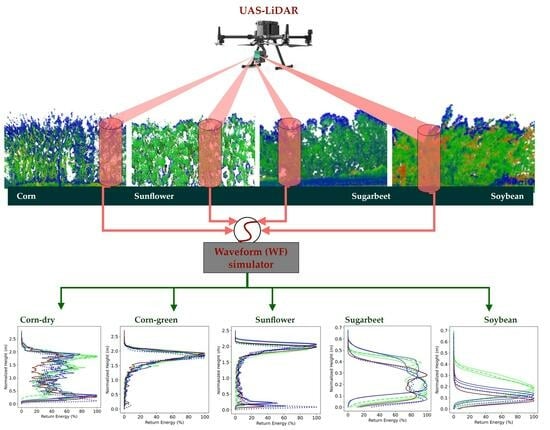
To understand external factors influencing the LiDAR backscatter, crop characteristic ULS waveform (WF) analysis is performed using multi-temporal simulated WFs [16,55]. WF analysis is designed to address the following: (i) do WFs show the characteristic WFs of corn, sunflower, soybean, and sugar beet, and in multi-temporal WFs; and (ii) does phenology influence the WF shapes, resulting in crop height differences over different crop successional stages? We aimed to consider all internal, e.g., flight altitude, PRR, scanning, and return echo modes, and external factors, e.g., crop type, structural complexity, and phonological stages.

(d)

Finally, regarding the vertical information loss for ULS WFs over agricultural environments, a comparative assessment is made with benchmark TLS WFs that provide concurrent detailed vegetation structural information [56,57,58].

To the best of our knowledge, assessing ULS operational parameters in the context of internal and external factors influencing LiDAR backscatter over soft targets, e.g., vegetation in agricultural settings using simulated WFs is lacking in past studies [27,54]. The existing methods for WF data calibration, data processing to plant properties retrieval have gradually been available yet are far from being mature [16]. Nonetheless, the present research establishes a generalized benchmark framework for ULS operational parameter optimization in an agricultural context using simulated WFs.

2. Materials and Methods

2.1. Study Area

This study was carried out over an experimental research area of 6597.60 m² centered at (96°49′20″W, 46°43′20″N) with a flat landscape, the elevation of which ranges from 277.50 m to 277.80 m above mean sea-level (M.S.L) in West Fargo, North Dakota, United States (see Figure 1a,b). The experiment included repeated LiDAR and VHR imagery observations of corn (Zea mays L.), soybean (Glycine max), sugar beet (Beta vulgaris L.), and sunflower (Helianthus annuus L.) of stagnant growth and changing phenology when crops were approaching their harvest dates. Moreover, the same crop with different phenological states offers a unique opportunity to evaluate the multi-temporal ULS point clouds over diverse crop environments, e.g., dry and green corn (Figure 1c). Moreover, a substantial portion of the chosen study site consists of bare ground, allowing for the LiDAR bare-ground point cloud evaluation in an agricultural context (Figure 1c). The selected sites contain weeds and shrubs among crops appropriate to ascertain the ULS mapping capabilities over fully vegetated and semi-vegetated landscapes, i.e., ground partially covered with weeds/grasses [25].

2.2. Data Collection

2.2.1. ULS Survey

DJI Matrice 300 RTK onboard optical and LiDAR sensors were used for repeated UAS surveys (Figure 1e–g). The DJI Zenmuse L1 equipped with a Livox laser sensor operating at the wavelength (λ) 1064 nm in near-infrared (NIR) is used to perform ULS surveys over experimental research sites following the designated flight mission (Figure 1d) [32]. Figure 1d illustrates multiple ULS surveys conducted on a single date, as detailed in

Table 1. ULS operational parameters setting for DJI Zenmuse L1 campaigns for early, intermediate, and late successional stages.

Stage	Echo Mode	Date	Frequency (kHz)	Scanning Mode	UAS Flight
					Altitude	Strip Overlap (%)	Speed (m/s)
Early	1	22 September 2022	160	Repetitive	50	50	5
	2	22 September 2022	160	Non-Repetitive	50	50	5
	3	22 September 2022	260	Repetitive	60	50	5
Intermediate	1	26 September 2022	160	Repetitive	50	50	5
	2	26 September 2022	160	Non-Repetitive	50	50	5
	2	26 September 2022	260	Repetitive	50	50	5
Late	2	27 September 2022	260	Repetitive	60	50	5

. To investigate the influence of crop orientation on acquired point clouds, UAS flight directions such as north to south (NS), east to west (EW), northeast (NE) to southwest (SW), and southeast (SE) to northwest (NW) were specifically designed. This was important to assess whether directional impact is evident in acquired point clouds or not. The survey was carried out at two designated altitudes, i.e., 50 m and 60 m above ground level (AGL) with a flight speed of 5 m/s and strip overlap of 50% following a similar approach [23,46]. Furthermore, a PRR of 160 kHz and 260 kHz along with one return echo (1n), two return echoes (2n), and three return echoes (3n) within each laser footprint were selected. The details of ULS operational parameters are given in Table 1 [32,46]. In addition, ULS surveys were conducted on three different dates to assess the temporal offset on multi-temporal point clouds. Red–green–blue (RGB) camera was operated simultaneously to collect VHR optical imagery aiding the ULS data analysis and visualization (Figure 1b,c) [8]. Moreover, the LiDAR sensor operated at a fixed nadir-looking angle for all ULS campaigns to avoid differences associated with scan zenith angle (SZA) distributions, and spherical losses [54]. Compared with ALS flying at much higher altitudes, e.g., 750 m AGL [54], ULSs flying at 50 m–60 m AGL, SZA, and spherical losses are trivial given that the LiDAR sensor is operated at a fixed nadir-looking configuration.

All UAS flights were performed within a time window (12:00–14:00 UTC) under clear sky conditions with comparable air temperature, humidity, visibility, wind speed, and solar elevation to minimize the possible offset of environmental factors on the geometric and radiometric properties of multi-temporal ULS data [54]. Consequently, the differences in LiDAR backscattered for different dates can be associated with geometric–optical properties of changing crop phenology and ULS operational practices. Three ULS surveys on 22 September 2022, 26 September 2022, and 27 September 2022, were classified as early, intermediate, and late successional stages, respectively. The connotation of early, intermediate, and late successional stages is used to explain the phenological influences on the multi-temporal ULS data. Hence, the given classification would not be mistaken for the actual crop growth stages which were stagnant during the ULS surveys (Table 1).

2.2.2. GNSS Field Survey

To establish the quality control (QC) of ULS derivative products, e.g., multi-temporal CHM, a GNSS field survey was carried out using a Trimble Geo7X differential survey-grade GPS unit to measure the geographic coordinates of each sampling point for different crops, e.g., dry corn, green corn, soybean, sugar beet, and sunflower [59,60]. GPS-based height measurements are subject to systemic height error further compounded by geographic and vertical geodetic transformation resulting in height error of fewer centimeters (cm) [61]. To achieve the best in situ height accuracy, crop heights were manually measured at each sampling location using a standard measuring pole (see Figure 2d). A minimum of three observations at each sampling location were made to ensure height accuracy, thereby eliminating the probability of human error. To minimize crop intrusion leading to plant structural damages, the crop’s in situ height measurements were taken from locations that offered easy access to sampling locations, e.g., voids in agricultural plots, walkways, row spacing, and plot boundaries (see yellow dots in Figure 1c).

The sampling points were then used to extract basic statistics, i.e., maximum, minimum, mean, and standard deviation of crop heights.

Table 2. Descriptive statistics of in situ crop height observations using GNSS and standard measuring pole.

Crop	No of Obs.	Crop Height (m)
		Minimum	Maximum	Mean	Standard Deviation
Green corn	10	2.14	3.03	2.49	0.30
Dry corn	6	2.15	2.94	2.60	0.30
Soybean	16	0.62	1.00	0.81	0.11
Sugar beet	11	0.37	0.75	0.58	0.11
Sunflower	14	0.78	1.96	1.64	0.33

shows the total number of height observations for each crop. For taller crops, e.g., sunflower (n = 14), dry corn (n = 6) and green corn (n = 10), less plant height variability was recorded; more height observations were recorded for soybean (n = 16) which showed a higher height variability (Table 2). Past experiments have shown that several samples (n = 289) of a single crop on a single date have slight changes in minimum, maximum, mean, and standard deviation [18]. The basic crop height statistics, e.g., standard deviation found in line with past studies to ensure that the crop height data were normally distributed and not biased due to a lower sampling strategy [18,19,41].

2.2.3. Terrestial Laser Scanner

UASs are useful in application settings of wide area mapping to construct 2D and 3D descriptions of crop environments with unprecedented spatio-temporal coverage [10,18]. LiDAR and optical sensors suffer from geometric occlusions caused by plant stems, leaves, and branches [23]. Though geometric occlusions are more pronounced for optical sensors, a comparison with a standard benchmark, i.e., TLS, is necessary to quantify the information loss of ULSs [62]. TLSs have been witnessed as great tools to measure fine-scale vegetation attributes [56,63]. TLSs generally operate in PRS space (≈5–10 m), apart from terrestrial objects, and translates most structural details compared with sensors onboard UASs, thus have been used as a reference benchmark to assess ULS information loss [57,64,65].

In this study, we used Livox 40 horizon operating at the wavelength (λ) 1064 nm in near-infrared (NIR) (Figure 1f)—an affordable LiDAR unit in static mode to acquire 3D point clouds at pre-selected locations of each crop, as shown in Figure 1c. Terrestrial scanners are frequently deployed in two modes: (a) mounted over a vehicle/moving platform, and (b) attached to a stationary fixed station, e.g., a tripod. The Livox 40 horizon only offers a non-repetitive mode. However, TLS being operated in static and non-repetitive mode can acquire far denser point clouds by scanning the same scene for a longer time than its counterpart ULS. Acquired TLS point clouds over dry corn, green corn, sunflower, sugar beet, and soybean are shown in Figure 2a–e. Using the reference scale, we assessed the height (z) accuracy of TLS point clouds of 2 mm when all TLS stations were placed approximately 5 m apart from the agricultural plots (see Figure 1c). Detailed descriptive statistics of acquired point clouds are provided in

Table 3. TLS operational parameters along with descriptive statistics of acquired points over five representative crops.

ID	Scanning Mode	Crop	Pts./m2	Wavelength	FOV	Range	Scan Mode	Range Accuracy
1	Spherical	Dry corn	9236.71	1064 nm	70.4 H: 77.4 V	200 m	Non-repetitive	2 mm
2	Spherical	Green corn	14,557.61	1064 nm	70.4 H: 77.4 V	200 m	Non-repetitive	2 mm
3	Spherical	Sunflower	4872.45	1064 nm	70.4 H: 77.4 V	200 m	Non-repetitive	2 mm
4	Spherical	Sugar beet	6072.14	1064 nm	70.4 H: 77.4 V	200 m	Non-repetitive	2 mm
5	Spherical	Soybean	8615.76	1064 nm	70.4 H: 77.4 V	200 m	Non-repetitive	2 mm

.

3. Methodology

3.1. Data Processing

First, all datasets (Figure 3a) were projected to Universal Transverse Mercator (UTM) coordinates zone 19N. In the pre-processing step, acquired VHR images were processed using the Pix4D mapping application to obtain orthophotos [66]. The ULS point clouds were obtained by processing DJI L1 raw data using the DJI Terra software application, and then strip adjustments between consecutive flight paths were performed to obtain seamless consistent ULS point clouds [25,54,67].

As shown in Figure 3b, TLS point clouds obtained using the Livox sensor were first registered with ULS point clouds obtained on the same date, i.e., 27 September 2022, using control points found in both datasets (see reference scale in Figure 2d) using CloudCompare (https://www.cloudcompare.org/, accessed on 30 November 2022)—an open-source software application [68,69]. For alignment, we used at least four solid targets located at different locations in the study area, e.g., light poles and reference scale bar (see Figure 2d). UAS-LiDAR equipped with Real Time Kinematic (RTK) provided the reference and TLS point clouds as registration targets. The outlier-noise points then were removed from the ULS and TLS point clouds using the statistical outlier removal (SOR) filter implemented in CloudCompare [25,70]. The quality of CHM is directly influenced by the quality of corresponding derivative products, i.e., DEM and DSM [71]. Multi-temporal ULS point clouds were classified into ground and non-ground points using the previously published author’s trained PointCNN model to achieve high classification accuracy [25]. In addition, a thorough ground point QC was performed to improve the classification results due to some limitations of the PointCNN model previously mentioned by authors [25]. TLS ground points were manually classified since the PointCNN model was trained for ULS ground point classification, and thus were not suitable for TLS data. Furthermore, TLS point clouds cover a smaller area of five representative sites (Figure 1c); therefore, accurate classification similar to ULS was accomplished using the ArcGIS desktop software application [25]. Height normalizations of ULS and TLS point clouds were performed using the lidR programming package [72].

3.2. Derivative Products

CHM are frequently used to estimate crop height metrics of individual plants or area-based approaches [36]. A CHM is constructed by subtracting a DEM from DSM, allowing the ground reference to be set to zero so that the plant’s equivalent heights with reference to in situ crop heights can be computed [73]. Multi-temporal CHM were developed at a fixed 0.12 m grid resolution using the lidR package [25,60,72,74]. The 0.12 m CHM is generated using a pit-free algorithm which ensures that the generated CHM do not suffer from no data values [75]. Through experiments, we found that CHM at 0.12 m grid size provides the highest resolution without data voids (pits) in the CHM raster [72].

3.3. Simulated ULS/TLS WFs

Point clouds are discrete measurements of crop vertical structures compared with LiDAR (WFs), which captures more information within the laser footprint than the discrete return mode [16]. Despite its usefulness, LiDAR WF data is comparatively more rare than point clouds [76]. Nonetheless, aerial and space-borne WF data are well known for forestry applications and have been rarely used in an agricultural context [16,77,78]. Lacking ULS-WFs, we simulated WFs for quality control and a 3D crop characterization framework over agricultural fields using multi-temporal point clouds [79]. A Python-based model simulating the WFs was developed using a similar approach [76]. The WF simulation process is described in Equations (1) and (2).

$$y=I\left(z\right)\ast G(m,n)$$

(1)

$$G(m,n)={\sum }_{i=1}^m{\sum }_{j=1}^n{e}^{-\frac{d_{ij}^2}{{2\sigma }^2}}{e}^{-\frac{{(x}_i-h_j)2}{{2\sigma }^2}}$$

(2)

In plain text language, y represents the simulated WF within the user-defined footprint. $I\left(z\right)$ represents the Lidar point cloud intensity convolution, i.e., the sum of Gaussian functions $G(m,n)$. The Gaussian convolution is performed within the footprint diameter for all reflecting surfaces (j-n) for all vertical energy bins (i-m). For example, $\left(h_j\right)$ is the elevation of $j^{th}$ reflecting surface located at a distance $\left(d_j^{}\right)$ from the center of the user-defined footprint. A detailed mathematical formulation of WF simulation can be found at [76]. Frequently, for simulation purposes, simplified synthetic plant models are developed [80]. To depict more realistic WFs, various studies directly use point clouds for simulation purposes instead of unrealistic synthetic plant models [76].

In our simulation framework, each point (x, y, z, i) in the point clouds is a reflecting surface of elevation (z) and intensity (i) that contributes to the WF simulation within a 1 m footprint. The simulation was accomplished for the ULS and TLS point clouds of corn, soybean, sugar beet, sunflower, and the ground partially covered with weeds/grasses [25,46,81]—see Figure 3b. Moreover, the simulations were conducted at specific site locations where ULS and TLS point clouds overlap with in situ field data to ensure that crop-specific height correlation and ULS information loss can be quantified meaningfully (see blue dots in Figure 1c). Given the fact that the ULS and TLS high-density point clouds experienced a moderate level of noise point clouds (see Figure 2), which were challenging to eliminate using traditional noise filtering approaches, e.g., SOR [25,70], Gaussian smoothing was performed to obtain the valid LiDAR echoes, i.e., peak amplitudes from the top, middle, and bottom of the canopy (Figure 4a,b)—a well-known approach in aerial and space-borne LiDAR WF data processing [16,77].

3.4. Evaluation Approaches

3.4.1. Multi-Temporal CHM Analysis

As shown in Figure 3c, a time-series CHM-based crop height analysis was performed using in situ crop height using a linear regression model (R²) [19]. Moreover, the root mean square error (RMSE)—Equation (3)—and mean absolute error (MAE)—Equation (4)—were computed, where n is the total number of observations, yᵢ is the in situ crop height measured using GNSS, and ŷᵢ is the crop height obtained from the CHM. To mitigate any GNSS signal offset in the geographic location of in situ crop height yᵢ, a 1 m buffer was used to find the best-fit ŷᵢ from time series CHM.

RMSE = √ (1/n Σ (yᵢ − ŷᵢ)²)

(3)

MAE = 1/n Σ|yᵢ − ŷᵢ|

(4)

3.4.2. Multi-Temporal WF Analysis

To quantify the vertical changes for multi-temporal simulated WFs, crop relative height (RH) metrics, i.e., the WF energy quartiles approach is used [80]. Figure 5 shows that RH metrics quantify the vertical distribution of laser pulse energy along the signal path at different elevations above mean sea level (M.S.L) by taking the ground peak amplitude as a reference [82,83,84]. For example, RH25 represents 25% of the total return energy above the ground peak amplitude, as depicted in Figure 5a–e [82]. The Gaussian decomposition (GP) method was used to find the ground peak amplitude in simulated WFs (see red line in Figure 5a–c) [82]. Pure ground WFs were also simulated using only bare-ground points (see Figure 5f) and used as a ground reference peak amplitude for RH metric calculations when ground peak amplitude is weak or invisible in simulated crop-specific WFs, which cannot be resolved with the GP method. For example, ground peak amplitude (solid-red-line) is missing for sugar beet (Figure 5d) and soybean (Figure 5f) where pure ground WFs were used for RH metric calculations (see Figure 5f) [82]. To establish the multi-temporal WFs analysis, we used RH10, RH25, RH50, RH75, and RH98 extracted from multi-temporal simulated WFs of dry corn, green corn, sugar beet, sunflower, and soybeans, which represent the 10%, 25%, 50%, 75%, and 98% return signal energy above the ground peak amplitude, as shown by the dotted green lines in Figure 5a–e. RH100 was excluded from the analysis as it was found to be biased due to some degree of noise at the leading edge of the LiDAR signal. Past studies have shown that RH98 is a suitable alternative to RH100 (Figure 5a–e). The RH metrics selection is based on their frequent use in previous studies [49,82]. RH metrics are generally used for AGB estimation using ALS and space-borne WFs Li-DAR data [49,82,85,86].

For an ideal scenario, multi-temporal ULS surveys over the same area of stagnant crop growth would result in insignificant differences in RH metric statistics of mean, median, and standard deviation, given that the ULS operational parameters and geometric–optical characteristics of the canopy remain unchanged for early, intermediate, and late successional crop stages. Subsequently, changes in ULS operational parameters and/or geometric–optical characteristics of crop environment would result in significant differences in RH metric statistics for multi-temporal ULS surveys. For the first time, we aim to use RH metrics to quantify the differences in multi-temporal simulated WFs using RH metrics. We calculated the statistics of minimum, maximum, mean, median, and standard deviation to quantify the change in multi-temporal ULS point clouds originating due to ULS operational practices in conjunction with changing phenology.

4. Results

4.1. Point Density Analysis

Point density is a quantitative measure of acquired point clouds, i.e., the number of points/m² [46].

Table 4. Descriptive statistics of acquired point clouds using different ULS operational parameters.

ID	N Mode	Date	PRR (kHz)	Scanning Mode	Altitude (AGL)	Pts./m2	Total pts (Millions).
Early	1	22 September 2022	160	Repetitive	50	590.82	4.00
	2	22 September 2022	160	Non-Repetitive	50	345.00	2.34
	3	22 September 2022	260	Repetitive	60	533.31	3.70
Intermediate	1	26 September 2022	260	Repetitive	50	912.17	6.18
	2	26 September 2022	160	Non-Repetitive	50	285.04	1.93
	2	26 September 2022	160	Repetitive	50	609.64	4.13
Late	2	27 September 2022	260	Repetitive	60	473.31	3.20

illustrates the point densities obtained from different ULS operational parameters. The point densities were quantified in the context of the ULS flight altitude, PRR, scanning modes, and return echoes modes, respectively.

At the altitude of 50 m AGL, with PRR = 160 kHz, scanning mode = repetitive, the acquired ULS point clouds at the early successional stage at (1n), and point clouds at the intermediate successional stage (2n), resulted in total points of 4.00 million and 4.13 million with point densities of 590.82 pts./m² and 609.64 pts./m², respectively. Taking the phenological losses into account, the observed point density at the intermediate successional stage must be lower than the early successional stage. Nonetheless, the results show that when the rest of the operational parameters were fixed, the (2n) yielded a point density a little higher at the intermediate than the (1n) at early successional stages. Moreover, at the same altitude, i.e., 50 m with (PRR = 160 kHz), (2n), the non-repetitive scanning mode at the early successional stage compared with the repetitive mode at the intermediate successional stage resulted in point densities of 328.81 and 609.64, respectively. We found that the repetitive scanning mode yields significantly higher point densities than the non-repetitive scanning mode. In the context of the changing ULS altitude (AGL), the acquired point clouds at 50 m and 60 m resulted in point densities of 912.17 pts/m² and 533.31 pts/m², given that the ULS operational parameters remained unchanged. The significant differences in the point densities at the different altitudes indicated that the altitude is a sensitive ULS operational parameter. The reflectance is associated with the sensor’s altitude, with higher altitudes giving a lower reflectance from the same target objects—soft (e.g., vegetation) and hard (man-made paved surfaces) targets [23]. We also found that the ULS with the (3n) configuration receives no more than two peak amplitudes over crop environments; therefore, operating DJI L1 with the (3n) mode yields similar point densities as the (2n) mode over agricultural plots. Our results indicate that the scanning mode and ULS operational altitudes were found to be more sensitive toward point densities over crop environments. Among the PRR configurations, 260 kHz yielded higher point densities than 160 kHz (see Table 4). This is likely that a higher PRR was found to be more effective in combating occlusion effects [23].

In the context of external factors influencing the acquired point clouds, at 50 m altitude with the return echo mode (2n), PRR = 160 kHz, and the non-repetitive scanning mode at the early and intermediate successional stages, resulted in point densities of 345.00 pts/m² and 285.40 pts./m², respectively. When all the ULS operational parameters were kept constant, there were higher point densities early compared to the intermediate successional stage, which is highly likely due to changes in the phenology of the given crop environments. A similar point density trend is found with constant operational parameters, i.e., altitude = 60 m, PRR = 260 kHz, and scanning mode = repetitive for dates early and late successional stages with point densities of 533.61 pts./m² and 473.31 pts./m², respectively. The point density analysis provided a general insight into the quantitative measure of acquired ULS point clouds (Table 4). Multi-temporal and spatio-temporal changes in point densities are therefore difficult to discern using point density analysis alone. To understand the impact of the ULS operational parameters, point densities, and return echo modes, a time series CHM analysis is documented in Section 4.2.

4.2. Multi-Temporal CHM Analysis

Table 4 shows that the ULS yields higher point densities regardless of flight altitudes, arguably providing rich information to generate VHR point cloud derivative products, e.g., DSM, DEM, and CHM [82]. This section therefore addresses the question of whether different operational parameters have an impact on ULS point cloud derivative products., e.g., time series CHM (see Figure 6).

The time series CHM in terms of the overall crop heights shows similar elevation ranges for the multi-temporal ULS dataset (Figure 6a–h). However, spatial changes in CHM were observed within the same period of ULS flights (see red rectangles and blue triangles in Figure 6a–c). Likewise, multi-temporal changes in crop heights were found to change over time, e.g., sugar beet and soybean showed a decreasing crop height over time (see white rectangles in Figure 6b,e,h). Such changes can be understood in the context of external and internal factors influencing the overall multi-temporal and spatio-temporal changes in the acquired point clouds.

Figure 6 illustrates that for the (2n) mode, the returns for the top of the canopy dominated the returns from the underlying ground compared with the (1n) mode, where the ground returns were more dominant than the crop surface reflectance (see blue triangles and red rectangles in Figure 6a,c) at an early successional stage. A similar behavior was observed in the intermediate successional stage where sugar beet, dry corn, and sunflower showed more ground returns for the (1n) mode compared with the (2n) mode (see red rectangles in Figure 6e,f), given that the other operational parameters, e.g., flight altitude, remained fixed. Also, (3n) showed a similar crop reflectance to (2n) for all the crops except sugar beet, where ground returns were selectively more pronounced (Figure 6a). Similarly, at a fixed altitude, i.e., 60 m, for the (3n) mode, the ground returns were more pronounced in the early successional stage over dry corn (Figure 6b) than in the intermediate successional stage (Figure 6d,e) for (2n) mode, respectively. Nonetheless, the (1n) and (3n) modes were found to provide deeper vegetation penetration than the (2n) mode regardless of the differences in data acquisition dates and altitudes (see blue triangles and red rectangles in Figure 6b,c,e,f). Quite the opposite, only two returns were registered for the (3n) mode yet with little deeper vegetation penetration than (2n) mode. Compared with the (2n) and (3n) modes, the (1n) mode provides the highest vegetation penetration for all the dates and operational parameters—an example is dry corn (see red rectangles in Figure 6c,f).

Overall, a general trend of more ground returns from the shorter crops is observed compared with the taller crops. Furthermore, the ground returns are more pronounced for the later dates than earlier dates (See blue and red rectangles in Figure 6d–h). The preliminary assessment of the ULS operational parameters using multi-temporal CHM analysis reveals two interesting findings. Firstly, the ULS operational parameters were found to be sensitive in terms of the canopy and corresponding ground returns. Secondly, with changing phenology, the ground returns were more pronounced for the shorter crops, yet it is not fully clear regarding the taller crops whether the ground returns were influenced by the ULS operational parameters or the changing phonologies of the given crop environments. Crop height underestimation was found to be significant for the shorter crops than the taller crops, as shown with the multi-temporal CHM analysis (Figure 6). Regardless of CHM’s frequent use, only the canopy heights and changes in the canopy heights can be understood using multi-temporal CHM analysis. To quantify the crop height discrepancy compared with in situ crop height measurements, a multi-temporal CHM height analysis is performed and presented in Section 4.3.

4.3. Crop Height Analysis

A linear regression was performed to understand the coefficient of determination (R²) between CHM and in situ crop heights [83]. Figure 7 illustrates that the overall multi-temporal CHM height showed good agreement with the in situ crop heights for the early, intermediate, and late successional stages. The results are in agreement with prior analyses [19,50].

Figure 7 shows that the overall correlation decreased when differences between the in situ crop heights and ULS campaigns increased. The crop heights were measured during the late successional stage on 27 September 2022. The overall strong correlation between the GNSS and CHM heights suggests that the crop height remained consistent for all the ULS campaigns. Moreover, given the fact that environmental factors remained unchanged for entire ULS campaigns (Section 2.2.1), the differences in R² (1.00–0.99), RMSE (0.04–0.09) m, and MAE (0.02–0.07) m are associated with phenological changes and ULS operational practices during this period (Figure 7a–c). Such differences are insignificant between consecutive flight campaigns (Figure 7b,c), indicative of a more pronounced effect of phonologies than operational parameters. However, crop-specific linear correlations, R², are important to understand the external factors influencing the quality and accuracy of multi-temporal ULS surveys. For that reason, the tall crop, e.g., corn and sunflower, and short crop, e.g., soybean and sugar beet, correlations with the field-measured heights were investigated.

4.3.1. Tall Crop Height Analysis

Figure 8 shows the overall coefficient of determination, R², between the in situ and tall crops’ CHM heights for the early, intermediate, and late successional stages. The linear correlation between the in situ and CHM heights showed a good agreement except for dry corn and green corn at the early successional stage. However, the correlation for the green corn height was found to be higher than that for the dry corn (see Figure 8a,d). The sunflowers showed the highest correlation between the in situ and CHM heights with the R² (0.99–1), RMSE (0.01–0.03) m, and MAE (0.01–0.02) m for all successional stages (Figure 8g–i). Our findings of the sunflower height estimates were in line with sensors’, e.g., multi-temporal optical and synthetic aperture radar (SAR) satellite data [84]. Sunflowers with stagnant flowering head growth for three different dates as observed in the field and height consistencies were expected, as observed in multi-temporal ULS data. A similar trend is illustrated for green corn (Figure 8d–f), where the (R² = 0.83–1), RMSE (0.01–0.08) m, and MAE (0.01–0.06) are observed for all successional stages. However, a large decrease is observed for green corn (R² = 0.83) for the ULS data collected in the early successional stage. A similar but higher discrepancy is observed for dry corn, with the (R² = 0.69), RMSE (0.03–0.10) m, and MAE (0.03–0.07) m. While the corn was at a mature growth stage, the discrepancy in the height correlation at the early successional stage occurred from either plant degradation or disorientation.

4.3.2. CHM-Based Short Crop Height Analysis

Figure 9c explains that soybeans showed a weak correlation (R² = 0.59) between the CHM and in situ plant height in the late successional stage (27 September 2022). However, the correlation (R² = 0.74–0.75) was found to be stronger for prior ULS surveys at the early (22 September 2027) and intermediate (26 September 2022) successional stages (Figure 9a,b). On the contrary, sugar beet showed a consistent correlation for all dates, with (R² = 0.97–1.00), RMSE (0.01–0.02) m, and MAE (0.01) m (see Figure 9d–f). The lower correlation for soybeans is caused by phenological changes, yet intertwined phenological changes and ULS operational parameters cannot be resolved using multi-temporal CHM analysis alone [19].

Figure 7, Figure 8 and Figure 9 demonstrate that the multi-temporal CHM compared with the in situ crop heights can help us to comprehend the overall and crop-specific coefficient of determination. Nonetheless, multi-temporal CHM analyses are purely based on the geometric distribution of crop point clouds; therefore, a deeper understanding of a particular crop response to LiDAR echoes is found to be challenging. Figure 6 shows that CHM can uncover spatio-temporal and multi-temporal crop height characteristics influenced by ULS operational practices and phenology. However, untangling the ULS operational practices and phenology impact on acquired point clouds using CHM analysis offers no clear explanation.

4.4. Multi-Temporal WF Analysis

Figure 10 demonstrates the multi-temporal simulated WFs of dry corn, green corn, bare ground, sugar beet, sunflower, and soybeans at a 1 m laser footprint. The WFs have typical multimodal characteristics, i.e., multiple peak amplitudes were observed from the top, middle, and ground of the crop environments, except for the ground and soybean, where the WFs were uni-modal. Figure 10 shows three distinct advantages of multi-temporal WF crop characterization over CHM-based analysis: First, the ULS-simulated WFs showed distinct WF signatures for dry corn, green corn, sugar beet, sunflower, soybean, and bare ground partially covered with weeds/grasses. Secondly, the WFs capture the vertical structural complexity, deciphering spatio-temporal changes more in depth than CHM (see Figure 6 and Figure 10). Thirdly, the simulated WFs reveal a clearer picture of the ULS operational practices over changing crop environments, where different sensor parameters showed a distinct impact on acquired point clouds. All three distinct aspects of the multi-temporal WF analysis are presented in the following subsections.

4.4.1. Crop Characteristic WFs

Figure 10 shows that the crop characteristic WFs are obtained using simulated WFs to depict the crop successional stages [78]. The number of peak amplitudes in the laser pulses show the responses of the different crops over a given time and LiDAR operational parameters. The taller crops, e.g., dry and green corn, show a distinct WF for the same date, differentiating the corns’ two distinct radiometric and geometric stages (Figure 10a,b). The portion of laser pulses reaching the ground was higher for the late successional stage than the early ULS surveys over the tall crops (Figure 10a,b,e). This is due to multiple scattering and absorption along the traveling path within the green corn causing information loss resulting in weak or no ground peak amplitudes (Figure 10b). On the contrary, dry corn showed a dissimilar LiDAR signal backscattered from the middle of the canopy and the ground (Figure 10a). Similarly, sunflowers exhibited bimodal characteristic WFs, i.e., the larger part of LiDAR backscattered from the top of the canopy and underlying soils (Figure 4b and Figure 10e). Figure 2 shows the point cloud 3D canopy closure at the late successional stage, which was better for dry corn and sunflowers than green corn with consistent phenology [54]. Green vegetation tends to reflect more in NIR at the 1064 nm wavelength, where the return energy peaks from the top of the green corn were about 100% (Figure 10b), compared with dry corn, which ranges between 60 and 100% with a decreasing trend for the intermediate and late successional stages (Figure 10a). On the contrary, for sunflowers, the peak amplitudes from the top of the canopy remained consistent for all the ULS campaigns yet increased ground returns were registered for the intermediate and late successional stages (Figure 10e). For sunflowers, the consistent flowering crown sizes throughout the ULS survey resulted in no change in the laser pulses from the top of the canopy (Figure 4b). However, with the changing leaf phenology, more ground returns were registered at the intermediate and late successional stages.

The bare ground with a small proportion of weeds and soybeans provided simplified unimodal WFs. The unimodal WFs depict that most of the LiDAR backscatter occurred from the ground (Figure 10c). The bare ground WF depicts weak peak amplitudes from the overlying weeds and grass compared with a single strong peak amplitude from the ground (Figure 10c). Soybeans depict truly unimodal characteristic WFs (Figure 9f). The most obvious difference between the ground and soybean WFs is the differences in the waveform length λ. The ground WFs were more compact in wavelength than those of the soybeans (Figure 10c–f). The broadening effect of the soybean WFs is highly likely due to the diffused LiDAR backscattered from the plants and underlying ground. For the multi-temporal WFs of soybean, the wavelength broadening effect linearly decreases from the early to the late successional stages, as shown with the shifting waveform wavelengths towards lower heights. This indicates that for the late successional stages, diffused LiDAR backscatter resolved to ground return peak amplitudes (see Figure 10c,f). The diffused LiDAR backscatter of the bare ground and soybean plants was challenging to classify as ground and non-ground points, as previously documented by authors [25]. The sugar beet characteristic WFs showed a unique behavior compared to the rest of the crops; the WFs’ shapes remained similar, i.e., typically bimodal for all successional stages, yet there was dissimilar WF orientation (see Figure 10d). This effect can be explained by sugar beets’ non-regular and non-Lambertian leaf surface [85], as shown with the field photos (Figure 13j,k). In addition, the ULS flight planning, as illustrated in Figure 1d, also influenced the LiDAR backscatter from the non-regular and non-Lambertian leaf surface of sugar beets. This critical information highlights the impact of directional scanning on ULS surveys over sugar beet fields (refer to Section 2.2.1). For consistent results, multi-temporal ULS surveys over sugar beet crops should maintain an identical flight line direction and sensor orientation to mitigate non-Lambertian behavior.

4.4.2. Crop Phenological Stages

Chlorophyll fluorescence, also known as the solar-induced fluorescence (SIF) content, increases over time. However, as crops approach their harvest, the photosynthesis rate and chlorophyll content start decaying. Photosynthesis not only changes spatio-temporally but also vertically at different rates for different crops. Optical remotely sensed datasets can reveal such changes in 2D space using traditional approaches, e.g., vegetation indices and fractional cover [86,87].

For the tall crops, Figure 10a showed that the dry corn experienced the most diverse LiDAR backscatter compared with its counterpart green corn, which showed a consistent response to ULS operational parameters over time (Figure 10b). Compared with green corn, dry corn shows that LiDAR backscatter is more dominant from the top of the canopy than the underlying soil for the first ULS survey at the early successional stage, as shown with the green lines, than the following ULS survey conducted in the intermediate and late successional stages, as shown with the blue and red lines in Figure 10a. Over time, with a changing phenology, the LiDAR backscatter decreased from the top of the canopy and increased from the underlying soil (see Figure 10a). On the contrary, green corn with an almost consistent chlorophyll content showed almost consistent backscatter for all the successional stages (Figure 10b). Similarly, sunflowers also indicated a similar trend in the LiDAR backscattered from the top of the canopy; however, the backscattering from the underlying soil became more dominant over time (Figure 10e).

For the short crops, e.g., soybean, a consistent shift in the crop height is observed over time, as shown with the green, blue, and red WFs in Figure 10f. This trend indicates changes in the phenological state of soybean, e.g., for an earlier successional stage, diffused LiDAR backscatter occurred, which resolved for the dominated ground peak amplitudes (see solid red lines in Figure 10c,f). A similar trend is visible for the LiDAR backscatter from the bare ground containing small weeds (Figure 10c). The present study therefore highlights the significance of using simulated WF ULS data to quantify the phenological stages of different crops given that the simulated WFs were generated by taking the laser echo intensity information into account [81]. For that reason, simulated WFs more effectively utilize the geometric and radiometric properties of terrestrial objects, e.g., vegetation [88].

4.4.3. Influence of ULS Operational Parameters

Table 4 summarizes the different ULS survey configurations to acquire high-density point clouds over different crop environments with rigorously changing crop phenology stages, i.e., from green to dry. In the context of ULS operational parameters, the single return (1n) and three return (3n) modes provided a deeper vegetation penetration compared with the double return (2n) mode (see dotted and dashed lines in Figure 10). On the contrary, the (2n) mode yields a higher number of returns from the top of the canopy than the (1n) and (3n) mode (see solid lines in Figure 10). Figure 6 shows that CHM has better crop heights modeled using the (2n) mode than (1n) and (3n) modes, thereby reflecting more crop surface features than the underlying ground. The field-acquired TLS point clouds depict that canopy gaps are insignificant for the shorter crops than the taller crop environments (Figure 4d,e). Therefore, row spacing and plant spacing distances become essential for the successful phenotyping of short crops using ULS data. In the context of elevation (z) accuracy evaluation for multi-temporal ULS datasets, there is a short offset between ULS point clouds acquired at the same date with different operational parameters. The offset can be attributed to the scan line error, which can be resolved by strip adjustment [25]; however, a small degree of offset remains in the processed LiDAR point clouds which is insignificant. For example, see the green lines in Figure 10f.

4.5. Statistical Change in RH Metrics

Figure 11 illustrates the graphical visualization of the quantitative change in the RH metrics of the multi-temporal simulated WFs, and descriptive statistics of the mean, median, minimum, maximum, and standard deviation are presented in

Table 5. Descriptive statistics of mean, median, minimum, maximum, and Std. Dev. For crop-specific RH metrics extracted from simulated WFs of multi-temporal ULS data. Figure 11 illustrates the graphical representation of RH metrics.

RH Metric	Crop	Mean	Median	Minimum	Maximum	Standard Deviation
RH10	Dry corn	5.37	5.77	0.98	8.01	2.43
	Green corn	9.99	10.12	8.87	10.48	0.50
	Soybeans	8.50	9.85	4.59	11.36	2.79
	Sugar beet	2.98	2.95	2.72	3.24	0.16
	Sunflower	7.33	6.99	3.42	10.12	2.24
RH25	Dry corn	19.99	20.02	14.20	22.99	2.92
	Green corn	25.22	25.33	24.22	25.89	0.47
	Soybeans	8.50	9.85	4.59	11.36	2.79
	Sugar beet	10.34	11.76	2.96	14.11	3.58
	Sunflower	21.94	21.89	14.48	25.13	3.40
RH50	Dry corn	45.05	45.03	38.98	47.98	3.04
	Green corn	50.34	50.28	49.55	51.29	0.56
	Soybeans	16.68	19.12	4.59	22.66	5.74
	Sugar beet	35.59	35.90	27.91	39.76	3.61
	Sunflower	47.37	47.63	38.96	51.70	3.81
RH75	Dry corn	69.99	69.97	63.93	72.97	3.07
	Green corn	75.76	75.75	74.41	77.31	0.84
	Soybeans	39.30	40.52	24.67	49.08	6.68
	Sugar beet	59.97	60.76	54.12	64.40	3.16
	Sunflower	73.04	72.96	63.91	76.82	3.97
RH98	Dry corn	92.86	92.89	86.86	95.82	2.99
	Green corn	97.91	98.05	96.85	98.27	0.45
	Soybeans	58.94	58.98	44.73	66.05	6.19
	Sugar beet	82.64	83.13	75.77	86.92	3.31
	Sunflower	94.96	94.90	86.86	98.61	3.62

. The energy distribution of the crops top-to-bottom showed two distinct patterns. For RH50 to RH98, a consistent and similar trend is depicted by all the crops (Figure 11c–e), which indicates that the top half of the crops showed a consistent change in the multi-temporal ULS campaigns for the three successional stages. For RH50-RH98, green corn showed the lowest differences in the geometric and radiometric response to LiDAR backscatter for the early, intermediate, and late successional stages (Figure 11c–e). The minor differences for green corn as indicated by the violin and box plots can be attributed to differences in the ULS operational parameters, e.g., the PRR, altitude, and scanning mode (Table 2). Sunflower and sugar beet showed similar shapes and sizes of the violin and box plots, indicating a consistent response to LiDAR incident pulses. However, the overall return energy budget was higher for sunflowers than sugar beet, respectively. On the contrary, a slightly higher return energy budget for dry corn than sugar beet can be attributed to differences in the volumetric responses, which are higher for dry corn than sugar beet. Meanwhile, for soybeans, the highest energy budget differences were found among all crops. The RH metrics revealed that the soybean response was substantially different within the vertical strata of the crops.

In terms of statistics, soybeans showed the highest standard deviation (5.74, 6.68, and 6.19) for the upper half of the canopies, i.e., RH50, RH75, and RH98, respectively. Dry corn, sunflower, and sugar beet showed similar trends with standard deviations within the range (2.99–3.97). On the other end, differences in the return LiDAR backscatter were lowered for sugar beet and green corn (see Figure 11a). Detailed descriptive RH metric statistics are provided in Table 5.

4.6. ULS Crop Characteristic Information Loss

Three-dimensional crop characterization from two different platforms, i.e., ULS and TLS, provides various insights into vegetation structure, deciphering the occlusion effect caused by the plant structural elements, leaf area, leaf orientation, and LAI [89,90]. Nonetheless, crop characteristic WF analysis was performed and compared with the TLS data acquired in the late successional stage to validate the following aspects of the ULS data: (a) Height (z) accuracy and consistency. (b) Information loss from the top, middle, and bottom of the canopies [90]. (c) Investigating crop characteristic WF differences. It should be noted that both ULS and TLS have onboard Livox laser sensors operating at 1064 nm; therefore, the direct comparison of sensor-specific WFs requires no additional laser intensity calibration/normalization at this stage of analysis.

4.6.1. Crop Height (z) Accuracy

The WF comparison between the ULS and TLS showed that both LiDAR sensors showed a consistent crop height accuracy for the taller crops, e.g., dry corn, green corn, and sunflower (Figure 12a–c). For the short crops, e.g., sugar beet and soybean, the ULS underestimated the crop heights compared with the TLS data (Figure 12d,e). Among all the crops, Figure 12e showed the highest information loss from the top of the canopies (0.4 m) observed for soybeans, which is evident from multi-temporal CHM and height correlation analysis (see Figure 6 and Figure 9a–c). Figure 12d shows that for sugar beet, the ULS ground peak has a broadening effect in wavelength compared to TLS; the broadening effect is due to the diffused LiDAR backscatter from plants and underlying ground for the ULS survey in the late successional state—a similar effect that was caused by slope surfaces on space-borne LiDAR WFs [80]. Figure 12e illustrates that the ULS and TLS ground peaks have good agreement, while the ULS experienced no peak amplitudes from the soybean canopy at the late successional stage. The multi-temporal ULS WFs in Figure 10e shows that the height underestimation is attributed to a differential phenology for entire ULS campaigns; however, past studies have shown that the TLS performance was not affected by phenological stages [64].

4.6.2. Information Loss Assessment

For the taller crops, e.g., green corn and sunflower, the information loss for the ULS from the middle of the canopy is more pronounced for green corn and sunflower compared to dry corn (Figure 12a–c). To quantify the response, from the middle of the canopy, the grey shaded area in Figure 12 indicates the (40–60)% portion of the return energy. The shaded grey area indicates that there were almost no strong peak amplitudes from the middle of the canopies for the ULS compared to the TLS (12a-c). For the short crops, a similar trend is found for soybean but contrasts for sugar beet, where the canopy tends to reflect more in the ULS than the TLS (see Figure 12d). This trend can be attributed to the leaf orientation as the leaf size stays the same within the same canopy over the same area. Past studies have shown that sugar beet leaf is non-Lambertian in terms of the surface reflectance [85]. Compared with the TLS, the ULS showed stronger peak amplitudes of the laser pulses over green corn and sunflower. It is likely that the ULS experiences less geometric occlusion than the TLS from the top of the canopy [91]. Most of the information loss for the ULS system is attributed to geometric occlusion caused by narrower rows and plant spacing. Therefore, reducing the information loss for the ULS, plant spacing, and row spacing are major contributing factors (see Figure 4).

4.6.3. Comparative Assessment of Crop Characteristic WFs

The ULS and TLS characteristics of the WFs showed similarities and differences, as illustrated in Figure 12. Dry corn experienced less geometric occlusion, and the characteristic WFs from the ULS and TLS showed similar shapes, yet the occlusion effects were found to be higher for the ULS than the TLS (see Figure 12a). On the contrary, green corn and sunflower experienced dissimilar occlusion effects, causing quite dissimilar WFs. The highest dissimilarity was found within the canopies where multiple strong peak amplitudes were registered for the TLS rather than ULS (see Figure 12b,c). Among the short crops, sugar beet showed typical bimodal WF shapes originating from the ULS and TLS (see Figure 12d). However, due to the leaf size and leaf angle of orientation, a more pronounced LiDAR backscatter peak amplitude from the top of the canopy is observed for the ULS than the TLS [85]. A typical soybean crop characteristic WF was found using the TLS (see Figure 12e) compared with the ULS, which provided unimodal characteristic WFs for all the ULS campaigns (see Figure 10e). This is due to the reason that almost all the ULS laser pulses were lost from the top of the soybean canopy and even quite weak peak amplitudes (i.e., return energy < 25%) were registered by the TLS stationed 5 m away from the canopy (see Figure 1c). The LiDAR backscattered from the ground showed similar coinciding peak amplitudes for the ULS and TLS, representing ground returns for all the crops (Figure 12a–e). However, the ground peak amplitudes were found to be weakest for green corn (Figure 12b) and diffused for sugar beet (Figure 12d). The diffused LiDAR backscatter occurs when the vertical distance between the sugar beet leaves and the ground is lower than the LiDAR range resolution. The range resolution is a common problem with ALS data to generate high-accuracy DEM and is generally caused by low foliage, bushes, and sub-shrubberies [92].

5. Discussion

CHM analysis has been frequently used to assess the agreement between LiDAR-measured and in situ crop heights [19,50]. This has been a classical approach to quantify the underestimation of crop heights measured using ULS [18,19,50]. We showed that the crop height underestimation for multi-temporal LiDAR occurred due to crop phenology, e.g., soybean and sugar beet (Figure 13g–k).

For multi-temporal ULS campaigns, phenological changes are responsible for differences in radiometry and geometry given the fact that radiometry and geometry are intertwined in LiDAR RS [54]. Therefore, height underestimation, specifically short crops, e.g., soybeans and sugar beet, was substantially caused by differential phenology rather than the ULS operational practices, which was cross-validated using a TLS (see Figure 12d,e). In theory, the ULS should result in similar heights for the different crops, yet the height underestimation is notably dissimilar for the tall and short crops (see Figure 8 and Figure 9). The field photos are indicative that the crop phenology has substantially changed while the heights remained almost similar, e.g., soybean in Figure 13h,i. Consequently, the height estimation of a particular crop, e.g., soybean was indicative of apparent changes that could be falsely attributed to actual changes in the crop height using multi-temporal ULS data [18,19,50]. We showed that the multi-temporal CHM analysis must be performed with caution, taking the radiometric–optical properties into account. Figure 12 shows that the late-season ULS data collection contributes to substantial errors in the data analysis (Figure 6e,f) due to the selective underestimation of a particular crop gene (Figure 8). Past studies have indicated a weaker correlation of the short crop heights compared with the ground truth, yet have not reached a reasonable conclusion [19]. Therefore, with multi-temporal simulated ULS WFs, phenological changes can be quantified in 3D space (see Figure 11).

Figure 13. Multi-temporal ULS point clouds with RGB coloring and intensity information for (a) early, (b) intermediate, and (c) late successional stages. The RGB coloration of point clouds indicates the difference in phenology at a different time, while intensity information describes the radiometric–optical changes over time, with deep brown representing lower reflectance at 1064 nm and bright colors indicating higher reflecting crops. (d) Field photo of dry corn in early, (e) dry corn in late, and (f) green corn in late successional stages. (g) Soybean at early, (h) at intermediate, and (i) at late successional stages. (j) Sugar beet at early and (k) late successional stages.

Figure 13. Multi-temporal ULS point clouds with RGB coloring and intensity information for (a) early, (b) intermediate, and (c) late successional stages. The RGB coloration of point clouds indicates the difference in phenology at a different time, while intensity information describes the radiometric–optical changes over time, with deep brown representing lower reflectance at 1064 nm and bright colors indicating higher reflecting crops. (d) Field photo of dry corn in early, (e) dry corn in late, and (f) green corn in late successional stages. (g) Soybean at early, (h) at intermediate, and (i) at late successional stages. (j) Sugar beet at early and (k) late successional stages.

Topographic LiDAR sensors are objectively designed to operate in the near-infrared (NIR) portion of the electromagnetic spectrum (EMS), whereas healthy vegetation has a higher reflectance and low transmittance in the NIR region; therefore, most of the transmitted laser pulses are backscattered, e.g., green vegetation (see black rectangles in Figure 6a–h and Figure 13a–c). For that reason, LiDAR sensors operational in the NIR regions would have greater influences on the height underestimation of the changing phenology in crop environments [86,87]. In PA, a multispectral or dual wavelength ULS can solve the selective underestimation of crop heights [1,10,65]. The other contributing factors, e.g., leaf size, shape, and leaf angle of orientation are the contributing factors toward height underestimation, e.g., the soybean leaf size is substantially smaller than sugar beet, contributing more towards height underestimation (Figure 12e and Figure 13g–i). However, this change is more serious near the harvest dates than the earlier dates, as shown with the multi-temporal WFs (Figure 10f). The crop’s spectral behavior therefore can be quantified with multi-temporal WF analysis alone (Figure 10 and Figure 12).

On the data processing end, CHM analysis involves point cloud classification, e.g., crop and ground points [19,25,74]. Ground points are then used for derivative products, e.g., DEM/DTM, DSM, and CHM. Inaccurate ground point classification highly likely contributes towards the under-/over-estimation of CHM heights when some of the crop points are classified as ground points or ground points are classified as crop points [25,47,49,93]. Furthermore, a wide variety of ground point classification algorithms have been developed; therefore, the choice and algorithm parameter optimization is a challenging task for ULS high-density point cloud classification [25]. The WF analysis showed that the LiDAR diffused backscatter from soybean and the underlying ground was challenging to differentiate between the ground and plant (see Figure 10f). To deal with diffused backscatter, bare-ground WFs (see Figure 10c) can be used as a valid reference to measure crop heights when the microtopography of the underlying crop surface is not important [93,94]. Our investigation showed that the CHM analysis has proven useful in deciphering the multi-temporal and spatiotemporal changes in crop height (Figure 6), however, an in-depth 3D crop vertical stratification is limited using the traditional CHM approaches.

Differential CHM, i.e., subtracting the early successional stage CHM from a late successional stage CHM have been used to quantify spatio-temporal changes in plant height, yet this approach does not account for vertical stratification within the canopies [95]. Figure 10 shows that WF analysis has been proven to be a robust approach to quantify spatio-temporal changes within the canopies. In the context of information loss, the TLS performs better than the ULS in crop environments with changing phenology. Though sugar beet and soybeans are short crops with comparable heights, both have significant differences in phenology, leaf sizes, and leaf orientations. A ULS operating at 50 m AGL suffers more information loss compared with a TLS operating at 5 m [23]. Nevertheless, a TLS operating at lower altitudes, e.g., 5 m, experiences more occlusions than a ULS operating at higher altitudes, e.g., 50 m. Our results were in line with past studies investigating crop height estimation using TLS data [64]. Particularly, short crop height estimation was found to be an effective approach by using TLS data for the entire growing season [96]. TLSs can effectively capture more ground and crop points over short crops, giving distinct peak amplitudes for plants and underlying ground, whereas for ULSs, diffused LiDAR backscatter was found over the short crops [40]. Generally, segmentation and classification in crop environments is a challenging task when multi-temporal ULS point clouds are available [25,97,98]. Thus, crop classifications and segmentation using crop characteristic WFs are one of the applications of the proposed 3D crop characterization framework.

Multiple returns echo, e.g., first, second, and third, can capture more information about the structure of the canopy and the ground surface [99]. For instance, the first return (1n) may represent the top of the canopy, while subsequent returns, e.g., (2n), (3n), may indicate mid-canopy or ground level. More complex vegetation structures, such as those with a dense canopy, will result in more varied return energy profiles across different return numbers. In the context of return from the ground, the highest peak amplitudes from the ground are observed for the (1n) mode with overall lower point densities (Table 4). Figure 10 illustrates that green corn (see Figure 13f) compared with dry corn (see Figure 13d,e) showed the least ground peak amplitudes for the (2n) and (3n) modes. The highest peak amplitudes from the ground are found against the (1n) mode (Figure 10b). This trend is true for the rest of the crop types (Figure 10a–f) including the ground returns from the ground surface (Figure 10c). Higher ground returns from underlying crops are useful to generate high-accuracy DEM models [93]. In the complex crop environment, DEM accuracy becomes important to generate accurate CHM (Figure 6). We showed that a ULS WF mode with a nominal footprint of 1 m can provide deeper crop penetration, registering more than three returns for tall crops and at least two returns for short crops (see Figure 10 and Figure 12). On the other end, a ULS discrete mode with a nominal footprint of 12 cm (e.g., DJI Zenmuse L1) is unable to provide more than two returns given the fact that the entire laser pulse is either reflected from the top, middle, or bottom of the canopies in rare cases where a pulse encounters two surfaces at different elevations, i.e., top of the canopy and ground [66]. Nonetheless, discrete ULSs are in frequent use to acquire point clouds in a wide area capacity at unprecedented spatio-temporal resolutions [25,27]. Currently, traditional approaches, e.g., point density/CHM have been adopted to extract crops’ structural attributes [18,19,49]. To this end, our investigation showed that the proposed benchmark workflow of simulated WFs therefore can fill this gap, i.e., the absence of a ULS WF mode. Likewise, the generalized benchmark simulated WF workflow advances the understanding and application of WFs LiDAR data, thereby setting the stage for a next-generation ULS WF mode [16,22,66].

In plant phenotyping, WF analysis reveals useful information to help one decide the plant spacing and row spacing so that optimal plant vertical stratification can be obtained using simulated WF-ULSs. Figure 13j,k show that sugar beet plants were tightly packed, causing substantial occlusions to incident laser pulses. For that reason, diffused LiDAR backscatter from the underlying ground occurred (Figure 10e). This study also investigated and showed that if the crop phenological stages remain the same (e.g., green corn), the vertical backscatter from the crop will remain almost unchanged (see Figure 10b and Figure 11). Finally, the RH metric statistical analysis showed that phenological influences are more pronounced than the ULS operational parameters (see Figure 11). Though phenological influences on ALS data have been investigated in the past [54], our study therefore sheds new light on phenological influences on ULS data.

6. Conclusions

In recent years, ULSs have advanced from custom-built prototypes to readily available survey-grade, turn-key precision agriculture (PA) solutions. In this article, we focused on multi-temporal ULS-simulated waveform (WF) analysis, which revealed significant insights into crop phenology and height estimation.

One of our key findings was that the multi-temporal ULS-simulated WF analysis explained the consistent crop height underestimation, especially during the intermediate and late successional stages. Moreover, our study highlighted that the shorter crops, e.g., soybeans, suffered more pronounced height underestimation compared to the taller crops, e.g., corn and sunflower. This selective height underestimation in the multi-temporal ULS data shed light on the impact of crop phenology on DJI Zemanse L1 operational practices. Traditional multi-temporal canopy height model (CHM) analysis, while informative about spatiotemporal changes in ULS point clouds, proved less effective in deciphering the individual influence of the ULS operational parameters and crop phenological changes.

Our research highlights that phenological influences have a more significant effect on acquired ULS point clouds than ULS operational practices. Subsequently, we recommend specific DJI L1 operational parameters, including a PRR of 260 kHz, the use of the repetitive scan mode, and the (2n) mode to achieve higher point densities from canopy tops in crop and grass environments. We found that the ULS point density analysis did not serve as the best proxy for assessing ULS operational practices compared with simulated WF analysis. The multi-temporal WF analysis, on the other hand, provided contradictory results in comparison to the traditional point density analysis. For example, the (1n) return echo mode yielded lower point densities but higher ground returns from underlying soils. This information proves instrumental when accurately deciphering underlying ground features, such as DTMs, and time series CHM analysis is important.

Nevertheless, ULS point clouds are frequently collected, and the use of WFs in agricultural contexts is an evolving approach. Our study therefore established a framework for simulating point clouds into WFs for crop 3D characterization. Although our research was based on DJI LI UAS laser scanning, the benchmark framework we developed can be applied to evaluate and assess the operational performance of other UAS laser scanning systems. We also found that consistent crop phenology in the study area resulted in almost identical WFs. However, variations arise when the crop’s radiometric–optical properties change over time, such as during phenological shifts. This insight can help establish a standardized timeline for ULS operations and data collection.

Additionally, we investigated the extent of information loss with ULS compared to Terrestrial LiDAR Systems (TLSs). Our study revealed that ULSs experience substantial information loss within canopies due to occlusions caused by plant stems, leaves, and branches. We concluded that designing appropriate row and plant spacing for phenotyping applications can mitigate the occlusion effect. Notably, broad-leaf plants, such as sugar beet, experienced more occlusion compared to small-leaf plants like soybeans.

While our study has provided new insights into ULS operations in crop environments, further experiments covering larger study areas with a wider variety of crop types are needed. Additionally, it is important to note that our investigation focused on multi-temporal ULS data using a fixed scanning angle from a nadir-looking LiDAR sensor. The impact of changing scanning angles on the acquired ULS point clouds remains unexplored in this article.

References

1. Rivera, G.; Porras, R.; Florencia, R.; Sánchez-Solís, J.P. LiDAR Applications in Precision Agriculture for Cultivating Crops: A Review of Recent Advances. Comput. Electron. Agric. 2023, 207, 107737. [Google Scholar] [CrossRef]
2. Weiss, M.; Jacob, F.; Duveiller, G. Remote Sensing for Agricultural Applications: A Meta-Review. Remote Sens. Environ. 2020, 236, 111402. [Google Scholar] [CrossRef]
3. Wendel, A.; Underwood, J.; Walsh, K. Maturity Estimation of Mangoes Using Hyperspectral Imaging from a Ground Based Mobile Platform. Comput. Electron. Agric. 2018, 155, 298–313. [Google Scholar] [CrossRef]
4. Comba, L.; Biglia, A.; Ricauda Aimonino, D.; Gay, P. Unsupervised Detection of Vineyards by 3D Point-Cloud UAV Photogrammetry for Precision Agriculture. Comput. Electron. Agric. 2018, 155, 84–95. [Google Scholar] [CrossRef]
5. Tao, H.; Xu, S.; Tian, Y.; Li, Z.; Ge, Y.; Zhang, J.; Wang, Y.; Zhou, G.; Deng, X.; Zhang, Z.; et al. Proximal and Remote Sensing in Plant Phenomics: 20 Years of Progress, Challenges, and Perspectives. Plant Commun. 2022, 3, 100344. [Google Scholar] [CrossRef] [PubMed]
6. Li, Q.; Jin, S.; Zang, J.; Wang, X.; Sun, Z.; Li, Z.; Xu, S.; Ma, Q.; Su, Y.; Guo, Q.; et al. Deciphering the Contributions of Spectral and Structural Data to Wheat Yield Estimation from Proximal Sensing. Crop J. 2022, 10, 1334–1345. [Google Scholar] [CrossRef]
7. Chang, C.Y.; Zhou, R.; Kira, O.; Marri, S.; Skovira, J.; Gu, L.; Sun, Y. An Unmanned Aerial System (UAS) for Concurrent Measurements of Solar-Induced Chlorophyll Fluorescence and Hyperspectral Reflectance toward Improving Crop Monitoring. Agric. For. Meteorol. 2020, 294, 108145. [Google Scholar] [CrossRef]
8. Jiang, S.; Jiang, C.; Jiang, W. Efficient Structure from Motion for Large-Scale UAV Images: A Review and a Comparison of SfM Tools. ISPRS J. Photogramm. Remote Sens. 2020, 167, 230–251. [Google Scholar] [CrossRef]
9. Zhou, J.; Khot, L.R.; Bahlol, H.Y.; Boydston, R.; Miklas, P.N. Evaluation of Ground, Proximal and Aerial Remote Sensing Technologies for Crop Stress Monitoring. IFAC-Pap. 2016, 49, 22–26. [Google Scholar] [CrossRef]
10. Müllerová, J.; Gago, X.; Bučas, M.; Company, J.; Estrany, J.; Fortesa, J.; Manfreda, S.; Michez, A.; Mokroš, M.; Paulus, G.; et al. Characterizing Vegetation Complexity with Unmanned Aerial Systems (UAS)—A Framework and Synthesis. Ecol. Indic. 2021, 131, 108156. [Google Scholar] [CrossRef]
11. Li, J.; Tang, L. Developing a Low-Cost 3D Plant Morphological Traits Characterization System. Comput. Electron. Agric. 2017, 143, 1–13. [Google Scholar] [CrossRef]
12. Sarić, R.; Nguyen, V.D.; Burge, T.; Berkowitz, O.; Trtílek, M.; Whelan, J.; Lewsey, M.G.; Čustović, E. Applications of Hyperspectral Imaging in Plant Phenotyping. Trends Plant Sci. 2022, 27, 301–315. [Google Scholar] [CrossRef] [PubMed]
13. Xie, C.; Yang, C. A Review on Plant High-Throughput Phenotyping Traits Using UAV-Based Sensors. Comput. Electron. Agric. 2020, 178, 105731. [Google Scholar] [CrossRef]
14. Hadaś, E.; Estornell, J. Accuracy of Tree Geometric Parameters Depending on the LiDAR Data Density. Eur. J. Remote Sens. 2016, 49, 73–92. [Google Scholar] [CrossRef]
15. An, N.; Welch, S.M.; Markelz, R.J.C.; Baker, R.L.; Palmer, C.M.; Ta, J.; Maloof, J.N.; Weinig, C. Quantifying Time-Series of Leaf Morphology Using 2D and 3D Photogrammetry Methods for High-Throughput Plant Phenotyping. Comput. Electron. Agric. 2017, 135, 222–232. [Google Scholar] [CrossRef]
16. Zhao, F.; Yang, X.; Schull, M.A.; Román-Colón, M.O.; Yao, T.; Wang, Z.; Zhang, Q.; Jupp, D.L.B.; Lovell, J.L.; Culvenor, D.S.; et al. Measuring Effective Leaf Area Index, Foliage Profile, and Stand Height in New England Forest Stands Using a Full-Waveform Ground-Based Lidar. Remote Sens. Environ. 2011, 115, 2954–2964. [Google Scholar] [CrossRef]
17. Rossi, R.; Costafreda-Aumedes, S.; Leolini, L.; Leolini, C.; Bindi, M.; Moriondo, M. Implementation of an Algorithm for Automated Phenotyping through Plant 3D-Modeling: A Practical Application on the Early Detection of Water Stress. Comput. Electron. Agric. 2022, 197, 106937. [Google Scholar] [CrossRef]
18. Gao, M.; Yang, F.; Wei, H.; Liu, X. Individual Maize Location and Height Estimation in Field from UAV-Borne LiDAR and RGB Images. Remote Sens. 2022, 14, 2292. [Google Scholar] [CrossRef]
19. Luo, S.; Liu, W.; Zhang, Y.; Wang, C.; Xi, X.; Nie, S.; Ma, D.; Lin, Y.; Zhou, G. Maize and Soybean Heights Estimation from Unmanned Aerial Vehicle (UAV) LiDAR Data. Comput. Electron. Agric. 2021, 182, 106005. [Google Scholar] [CrossRef]
20. Cucchiaro, S.; Straffelini, E.; Chang, K.-J.; Tarolli, P. Mapping Vegetation-Induced Obstruction in Agricultural Ditches: A Low-Cost and Flexible Approach by UAV-SfM. Agric. Water Manag. 2021, 256, 107083. [Google Scholar] [CrossRef]
21. Amarasingam, N.; Ashan Salgadoe, A.S.; Powell, K.; Gonzalez, L.F.; Natarajan, S. A Review of UAV Platforms, Sensors, and Applications for Monitoring of Sugarcane Crops. Remote Sens. Appl. Soc. Environ. 2022, 26, 100712. [Google Scholar] [CrossRef]
22. Nex, F.; Armenakis, C.; Cramer, M.; Cucci, D.A.; Gerke, M.; Honkavaara, E.; Kukko, A.; Persello, C.; Skaloud, J. UAV in the Advent of the Twenties: Where We Stand and What Is Next. ISPRS J. Photogramm. Remote Sens. 2022, 184, 215–242. [Google Scholar] [CrossRef]
23. Brede, B.; Bartholomeus, H.M.; Barbier, N.; Pimont, F.; Vincent, G.; Herold, M. Peering through the Thicket: Effects of UAV LiDAR Scanner Settings and Flight Planning on Canopy Volume Discovery. Int. J. Appl. Earth Obs. Geoinf. 2022, 114, 103056. [Google Scholar] [CrossRef]
24. Nowak, M.M.; Pędziwiatr, K.; Bogawski, P. Hidden Gaps under the Canopy: LiDAR-Based Detection and Quantification of Porosity in Tree Belts. Ecol. Indic. 2022, 142, 109243. [Google Scholar] [CrossRef]
25. Fareed, N.; Flores, J.P.; Das, A.K. Analysis of UAS-LiDAR Ground Points Classification in Agricultural Fields Using Traditional Algorithms and PointCNN. Remote Sens. 2023, 15, 483. [Google Scholar] [CrossRef]
26. Jurado, J.J.M.; López, A.; Pádua, L.; Sousa, J.J. Remote Sensing Image Fusion on 3D Scenarios: A Review of Applications for Agriculture and Forestry. Int. J. Appl. Earth Obs. Geoinf. 2022, 112, 102856. [Google Scholar] [CrossRef]
27. Lin, Y. LiDAR: An Important Tool for next-Generation Phenotyping Technology of High Potential for Plant Phenomics? Comput. Electron. Agric. 2015, 119, 61–73. [Google Scholar] [CrossRef]
28. Micheletto, M.J.; Chesñevar, C.I.; Santos, R. Methods and Applications of 3D Ground Crop Analysis Using LiDAR Technology: A Survey. Sensors 2023, 23, 7212. [Google Scholar] [CrossRef] [PubMed]
29. Sofonia, J.J.; Phinn, S.; Roelfsema, C.; Kendoul, F.; Rist, Y. Modelling the Effects of Fundamental UAV Flight Parameters on LiDAR Point Clouds to Facilitate Objectives-Based Planning. ISPRS J. Photogramm. Remote Sens. 2019, 149, 105–118. [Google Scholar] [CrossRef]
30. Maltamo, M.; Peltola, P.; Packalen, P.; Hardenbol, A.; Räty, J.; Saksa, T.; Eerikäinen, K.; Korhonen, L. Can Models for Forest Attributes Based on Airborne Laser Scanning Be Generalized for Different Silvicultural Management Systems? For. Ecol. Manag. 2023, 546, 121312. [Google Scholar] [CrossRef]
31. Mathews, A.J.; Singh, K.K.; Cummings, A.R.; Rogers, S.R. Fundamental Practices for Drone Remote Sensing Research across Disciplines. Drone Syst. Appl. 2023, 11, 1–22. [Google Scholar] [CrossRef]
32. Diara, F.; Roggero, M. Quality Assessment of DJI Zenmuse L1 and P1 LiDAR and Photogrammetric Systems: Metric and Statistics Analysis with the Integration of Trimble SX10 Data. Geomatics 2022, 2, 254–281. [Google Scholar] [CrossRef]
33. Adnan, S.; Maltamo, M.; Mehtätalo, L.; Ammaturo, R.N.L.; Packalen, P.; Valbuena, R. Determining Maximum Entropy in 3D Remote Sensing Height Distributions and Using It to Improve Aboveground Biomass Modelling via Stratification. Remote Sens. Environ. 2021, 260, 112464. [Google Scholar] [CrossRef]
34. Pedersen, R.Ø.; Bollandsås, O.M.; Gobakken, T.; Næsset, E. Deriving Individual Tree Competition Indices from Airborne Laser Scanning. For. Ecol. Manag. 2012, 280, 150–165. [Google Scholar] [CrossRef]
35. Wallace, L.; Lucieer, A.; Watson, C.; Turner, D. Development of a UAV-LiDAR System with Application to Forest Inventory. Remote Sens. 2012, 4, 1519–1543. [Google Scholar] [CrossRef]
36. Zheng, Z.; Schmid, B.; Zeng, Y.; Schuman, M.C.; Zhao, D.; Schaepman, M.E.; Morsdorf, F. Remotely Sensed Functional Diversity and Its Association with Productivity in a Subtropical Forest. Remote Sens. Environ. 2023, 290, 113530. [Google Scholar] [CrossRef]
37. Radoglou-Grammatikis, P.; Sarigiannidis, P.; Lagkas, T.; Moscholios, I. A Compilation of UAV Applications for Precision Agriculture. Comput. Netw. 2020, 172, 107148. [Google Scholar] [CrossRef]
38. Malambo, L.; Popescu, S.C.; Horne, D.W.; Pugh, N.A.; Rooney, W.L. Automated Detection and Measurement of Individual Sorghum Panicles Using Density-Based Clustering of Terrestrial Lidar Data. ISPRS J. Photogramm. Remote Sens. 2019, 149, 1–13. [Google Scholar] [CrossRef]
39. Bi, K.; Gao, S.; Xiao, S.; Zhang, C.; Bai, J.; Huang, N.; Sun, G.; Niu, Z. N Distribution Characterization Based on Organ-Level Biomass and N Concentration Using a Hyperspectral Lidar. Comput. Electron. Agric. 2022, 199, 107165. [Google Scholar] [CrossRef]
40. Hu, X.; Sun, L.; Gu, X.; Sun, Q.; Wei, Z.; Pan, Y.; Chen, L. Assessing the Self-Recovery Ability of Maize after Lodging Using UAV-LiDAR Data. Remote Sens. 2021, 13, 2270. [Google Scholar] [CrossRef]
41. Tian, Y.; Huang, H.; Zhou, G.; Zhang, Q.; Tao, J.; Zhang, Y.; Lin, J. Aboveground Mangrove Biomass Estimation in Beibu Gulf Using Machine Learning and UAV Remote Sensing. Sci. Total Environ. 2021, 781, 146816. [Google Scholar] [CrossRef]
42. Jin, C.; Oh, C.; Shin, S.; Wilfred Njungwi, N.; Choi, C. A Comparative Study to Evaluate Accuracy on Canopy Height and Density Using UAV, ALS, and Fieldwork. Forests 2020, 11, 241. [Google Scholar] [CrossRef]
43. Lin, Y.-C.; Cheng, Y.-T.; Zhou, T.; Ravi, R.; Hasheminasab, S.; Flatt, J.; Troy, C.; Habib, A. Evaluation of UAV LiDAR for Mapping Coastal Environments. Remote Sens. 2019, 11, 2893. [Google Scholar] [CrossRef]
44. Hu, T.; Sun, X.; Su, Y.; Guan, H.; Sun, Q.; Kelly, M.; Guo, Q. Development and Performance Evaluation of a Very Low-Cost UAV-Lidar System for Forestry Applications. Remote Sens. 2020, 13, 77. [Google Scholar] [CrossRef]
45. Zhang, Y.; Tan, Y.; Onda, Y.; Hashimoto, A.; Gomi, T.; Chiu, C.; Inokoshi, S. A Tree Detection Method Based on Trunk Point Cloud Section in Dense Plantation Forest Using Drone LiDAR Data. For. Ecosyst. 2023, 10, 100088. [Google Scholar] [CrossRef]
46. Štroner, M.; Urban, R.; Línková, L. A New Method for UAV Lidar Precision Testing Used for the Evaluation of an Affordable DJI ZENMUSE L1 Scanner. Remote Sens. 2021, 13, 4811. [Google Scholar] [CrossRef]
47. Bartmiński, P.; Siłuch, M.; Kociuba, W. The Effectiveness of a UAV-Based LiDAR Survey to Develop Digital Terrain Models and Topographic Texture Analyses. Sensors 2023, 23, 6415. [Google Scholar] [CrossRef]
48. Lao, Z.; Fu, B.; Wei, Y.; Deng, T.; He, W.; Yang, Y.; He, H.; Gao, E. Retrieval of Chlorophyll Content for Vegetation Communities under Different Inundation Frequencies Using UAV Images and Field Measurements. Ecol. Indic. 2024, 158, 111329. [Google Scholar] [CrossRef]
49. Hu, X.; Gu, X.; Sun, Q.; Yang, Y.; Qu, X.; Yang, X.; Guo, R. Comparison of the Performance of Multi-Source Three-Dimensional Structural Data in the Application of Monitoring Maize Lodging. Comput. Electron. Agric. 2023, 208, 107782. [Google Scholar] [CrossRef]
50. Shu, M.; Li, Q.; Ghafoor, A.; Zhu, J.; Li, B.; Ma, Y. Using the Plant Height and Canopy Coverage to Estimation Maize Aboveground Biomass with UAV Digital Images. Eur. J. Agron. 2023, 151, 126957. [Google Scholar] [CrossRef]
51. Wang, D.; Xing, S.; He, Y.; Yu, J.; Xu, Q.; Li, P. Evaluation of a New Lightweight UAV-Borne Topo-Bathymetric LiDAR for Shallow Water Bathymetry and Object Detection. Sensors 2022, 22, 1379. [Google Scholar] [CrossRef] [PubMed]
52. Appiah Mensah, A.; Jonzén, J.; Nyström, K.; Wallerman, J.; Nilsson, M. Mapping Site Index in Coniferous Forests Using Bi-Temporal Airborne Laser Scanning Data and Field Data from the Swedish National Forest Inventory. For. Ecol. Manag. 2023, 547, 121395. [Google Scholar] [CrossRef]
53. Zhou, C.; Ye, H.; Sun, D.; Yue, J.; Yang, G.; Hu, J. An Automated, High-Performance Approach for Detecting and Characterizing Broccoli Based on UAV Remote-Sensing and Transformers: A Case Study from Haining, China. Int. J. Appl. Earth Obs. Geoinf. 2022, 114, 103055. [Google Scholar] [CrossRef]
54. Korpela, I.; Polvivaara, A.; Hovi, A.; Junttila, S.; Holopainen, M. Influence of Phenology on Waveform Features in Deciduous and Coniferous Trees in Airborne LiDAR. Remote Sens. Environ. 2023, 293, 113618. [Google Scholar] [CrossRef]
55. Dalponte, M.; Jucker, T.; Liu, S.; Frizzera, L.; Gianelle, D. Characterizing Forest Carbon Dynamics Using Multi-Temporal Lidar Data. Remote Sens. Environ. 2019, 224, 412–420. [Google Scholar] [CrossRef]
56. Penman, S.; Lentini, P.; Law, B.; York, A. An Instructional Workflow for Using Terrestrial Laser Scanning (TLS) to Quantify Vegetation Structure for Wildlife Studies. For. Ecol. Manag. 2023, 548, 121405. [Google Scholar] [CrossRef]
57. Su, W.; Zhu, D.; Huang, J.; Guo, H. Estimation of the Vertical Leaf Area Profile of Corn (Zea Mays) Plants Using Terrestrial Laser Scanning (TLS). Comput. Electron. Agric. 2018, 150, 5–13. [Google Scholar] [CrossRef]
58. Xuming, G.; Yuting, F.; Qing, Z.; Bin, W.; Bo, X.; Han, H.; Min, C. Semantic Maps for Cross-View Relocalization of Terrestrial to UAV Point Clouds. Int. J. Appl. Earth Obs. Geoinf. 2022, 114, 103081. [Google Scholar] [CrossRef]
59. Yan, D.; Li, J.; Yao, X.; Luan, Z. Integrating UAV Data for Assessing the Ecological Response of Spartina Alterniflora towards Inundation and Salinity Gradients in Coastal Wetland. Sci. Total Environ. 2022, 814, 152631. [Google Scholar] [CrossRef]
60. Xu, W.; Yang, W.; Wu, J.; Chen, P.; Lan, Y.; Zhang, L. Canopy Laser Interception Compensation Mechanism—UAV LiDAR Precise Monitoring Method for Cotton Height. Agronomy 2023, 13, 2584. [Google Scholar] [CrossRef]
61. Zhang, Z.; Pan, L. Current Performance of Open Position Service with Almost Fully Deployed Multi-GNSS Constellations: GPS, GLONASS, Galileo, BDS-2, and BDS-3. Adv. Space Res. 2022, 69, 1994–2019. [Google Scholar] [CrossRef]
62. Beland, M.; Parker, G.; Sparrow, B.; Harding, D.; Chasmer, L.; Phinn, S.; Antonarakis, A.; Strahler, A. On Promoting the Use of Lidar Systems in Forest Ecosystem Research. For. Ecol. Manag. 2019, 450, 117484. [Google Scholar] [CrossRef]
63. Sun, J.; Lin, Y. Assessing the Allometric Scaling of Vectorized Branch Lengths of Trees with Terrestrial Laser Scanning and Quantitative Structure Modeling: A Case Study in Guyana. Remote Sens. 2023, 15, 5005. [Google Scholar] [CrossRef]
64. El-Naggar, A.G.; Jolly, B.; Hedley, C.B.; Horne, D.; Roudier, P.; Clothier, B.E. The Use of Terrestrial LiDAR to Monitor Crop Growth and Account for Within-Field Variability of Crop Coefficients and Water Use. Comput. Electron. Agric. 2021, 190, 106416. [Google Scholar] [CrossRef]
65. Guo, Q.; Su, Y.; Hu, T. The Origin and Development of LiDAR Techniques. In LiDAR Principles, Processing and Applications in Forest Ecology; Elsevier: Amsterdam, The Netherlands, 2023; pp. 1–22. ISBN 978-0-12-823894-3. [Google Scholar]
66. Jin, S.; Sun, X.; Wu, F.; Su, Y.; Li, Y.; Song, S.; Xu, K.; Ma, Q.; Baret, F.; Jiang, D.; et al. Lidar Sheds New Light on Plant Phenomics for Plant Breeding and Management: Recent Advances and Future Prospects. ISPRS J. Photogramm. Remote Sens. 2021, 171, 202–223. [Google Scholar] [CrossRef]
67. Willers, J.; Jin, M.; Eksioglu, B.; Zusmanis, A.; O’Hara, C.; Jenkins, J. A Post-Processing Step Error Correction Algorithm for Overlapping LiDAR Strips from Agricultural Landscapes. Comput. Electron. Agric. 2008, 64, 183–193. [Google Scholar] [CrossRef]
68. Shao, J.; Yao, W.; Wan, P.; Luo, L.; Wang, P.; Yang, L.; Lyu, J.; Zhang, W. Efficient Co-Registration of UAV and Ground LiDAR Forest Point Clouds Based on Canopy Shapes. Int. J. Appl. Earth Obs. Geoinf. 2022, 114, 103067. [Google Scholar] [CrossRef]
69. Letard, M.; Lague, D.; Le Guennec, A.; Lefèvre, S.; Feldmann, B.; Leroy, P.; Girardeau-Montaut, D.; Corpetti, T. 3DMASC: Accessible, Explainable 3D Point Clouds Classification. Application to BI-Spectral TOPO-Bathymetric Lidar Data. ISPRS J. Photogramm. Remote Sens. 2024, 207, 175–197. [Google Scholar] [CrossRef]
70. Wang, B.; Ma, Y.; Zhang, J.; Zhang, H.; Zhu, H.; Leng, Z.; Zhang, X.; Cui, A. A Noise Removal Algorithm Based on Adaptive Elevation Difference Thresholding for ICESat-2 Photon-Counting Data. Int. J. Appl. Earth Obs. Geoinf. 2023, 117, 103207. [Google Scholar] [CrossRef]
71. Nelson, A.; Reuter, H.I.; Gessler, P. Chapter 3 DEM Production Methods and Sources. In Developments in Soil Science; Elsevier: Amsterdam, The Netherlands, 2009; Volume 33, ISBN 978-0-12-374345-9. [Google Scholar]
72. Roussel, J.-R.; Auty, D.; Coops, N.C.; Tompalski, P.; Goodbody, T.R.H.; Meador, A.S.; Bourdon, J.-F.; De Boissieu, F.; Achim, A. lidR: An R Package for Analysis of Airborne Laser Scanning (ALS) Data. Remote Sens. Environ. 2020, 251, 112061. [Google Scholar] [CrossRef]
73. Dong, T.; Zhang, X.; Ding, Z.; Fan, J. Multi-Layered Tree Crown Extraction from LiDAR Data Using Graph-Based Segmentation. Comput. Electron. Agric. 2020, 170, 105213. [Google Scholar] [CrossRef]
74. Klápště, P.; Fogl, M.; Barták, V.; Gdulová, K.; Urban, R.; Moudrý, V. Sensitivity Analysis of Parameters and Contrasting Performance of Ground Filtering Algorithms with UAV Photogrammetry-Based and LiDAR Point Clouds. Int. J. Digit. Earth 2020, 13, 1672–1694. [Google Scholar] [CrossRef]
75. Khosravipour, A.; Skidmore, A.K.; Isenburg, M.; Wang, T.; Hussin, Y.A. Generating Pit-Free Canopy Height Models from Airborne Lidar. Photogramm. Eng. Remote Sens. 2014, 80, 863–872. [Google Scholar] [CrossRef]
76. Blair, J.B.; Hofton, M.A. Modeling Laser Altimeter Return Waveforms over Complex Vegetation Using High-resolution Elevation Data. Geophys. Res. Lett. 1999, 26, 2509–2512. [Google Scholar] [CrossRef]
77. Myroniuk, V.; Zibtsev, S.; Bogomolov, V.; Goldammer, J.G.; Soshenskyi, O.; Levchenko, V.; Matsala, M. Combining Landsat Time Series and GEDI Data for Improved Characterization of Fuel Types and Canopy Metrics in Wildfire Simulation. J. Environ. Manag. 2023, 345, 118736. [Google Scholar] [CrossRef] [PubMed]
78. Gu, Z.; Cao, S.; Sanchez-Azofeifa, G.A. Using LiDAR Waveform Metrics to Describe and Identify Successional Stages of Tropical Dry Forests. Int. J. Appl. Earth Obs. Geoinf. 2018, 73, 482–492. [Google Scholar] [CrossRef]
79. Di Tommaso, S.; Wang, S.; Vajipey, V.; Gorelick, N.; Strey, R.; Lobell, D.B. Annual Field-Scale Maps of Tall and Short Crops at the Global Scale Using GEDI and Sentinel-2. Remote Sens. 2023, 15, 4123. [Google Scholar] [CrossRef]
80. Wang, Y.; Ni, W.; Sun, G.; Chi, H.; Zhang, Z.; Guo, Z. Slope-Adaptive Waveform Metrics of Large Footprint Lidar for Estimation of Forest Aboveground Biomass. Remote Sens. Environ. 2019, 224, 386–400. [Google Scholar] [CrossRef]
81. Ranson, K.J.; Sun, G. Modeling Lidar Returns from Forest Canopies. IEEE Trans. Geosci. Remote Sens. 2000, 38, 2617–2626. [Google Scholar] [CrossRef]
82. Amini Amirkolaee, H.; Arefi, H.; Ahmadlou, M.; Raikwar, V. DTM Extraction from DSM Using a Multi-Scale DTM Fusion Strategy Based on Deep Learning. Remote Sens. Environ. 2022, 274, 113014. [Google Scholar] [CrossRef]
83. Jing, L.; Wei, X.; Song, Q.; Wang, F. Research on Estimating Rice Canopy Height and LAI Based on LiDAR Data. Sensors 2023, 23, 8334. [Google Scholar] [CrossRef]
84. Fieuzal, R.; Baup, F. Estimation of Leaf Area Index and Crop Height of Sunflowers Using Multi-Temporal Optical and SAR Satellite Data. Int. J. Remote Sens. 2016, 37, 2780–2809. [Google Scholar] [CrossRef]
85. Jay, S.; Bendoula, R.; Hadoux, X.; Féret, J.-B.; Gorretta, N. A Physically-Based Model for Retrieving Foliar Biochemistry and Leaf Orientation Using Close-Range Imaging Spectroscopy. Remote Sens. Environ. 2016, 177, 220–236. [Google Scholar] [CrossRef]
86. Seo, B.; Lee, J.; Lee, K.-D.; Hong, S.; Kang, S. Improving Remotely-Sensed Crop Monitoring by NDVI-Based Crop Phenology Estimators for Corn and Soybeans in Iowa and Illinois, USA. Field Crops Res. 2019, 238, 113–128. [Google Scholar] [CrossRef]
87. Yue, J.; Tian, J.; Philpot, W.; Tian, Q.; Feng, H.; Fu, Y. VNAI-NDVI-Space and Polar Coordinate Method for Assessing Crop Leaf Chlorophyll Content and Fractional Cover. Comput. Electron. Agric. 2023, 207, 107758. [Google Scholar] [CrossRef]
88. Mallet, C.; Bretar, F. Full-Waveform Topographic Lidar: State-of-the-Art. ISPRS J. Photogramm. Remote Sens. 2009, 64, 1–16. [Google Scholar] [CrossRef]
89. Malambo, L.; Popescu, S.C.; Murray, S.C.; Putman, E.; Pugh, N.A.; Horne, D.W.; Richardson, G.; Sheridan, R.; Rooney, W.L.; Avant, R.; et al. Multitemporal Field-Based Plant Height Estimation Using 3D Point Clouds Generated from Small Unmanned Aerial Systems High-Resolution Imagery. Int. J. Appl. Earth Obs. Geoinf. 2018, 64, 31–42. [Google Scholar] [CrossRef]
90. Zhao, X.; Su, Y.; Hu, T.; Cao, M.; Liu, X.; Yang, Q.; Guan, H.; Liu, L.; Guo, Q. Analysis of UAV Lidar Information Loss and Its Influence on the Estimation Accuracy of Structural and Functional Traits in a Meadow Steppe. Ecol. Indic. 2022, 135, 108515. [Google Scholar] [CrossRef]
91. Jaakkola, A.; Hyyppä, J.; Kukko, A.; Yu, X.; Kaartinen, H.; Lehtomäki, M.; Lin, Y. A Low-Cost Multi-Sensoral Mobile Mapping System and Its Feasibility for Tree Measurements. ISPRS J. Photogramm. Remote Sens. 2010, 65, 514–522. [Google Scholar] [CrossRef]
92. Ma, H.; Zhou, W.; Zhang, L. DEM Refinement by Low Vegetation Removal Based on the Combination of Full Waveform Data and Progressive TIN Densification. ISPRS J. Photogramm. Remote Sens. 2018, 146, 260–271. [Google Scholar] [CrossRef]
93. Liu, G.; Xia, J.; Zheng, K.; Cheng, J.; Wang, K.; Liu, Z.; Wei, Y.; Xie, D. Measurement and Evaluation Method of Farmland Microtopography Feature Information Based on 3D LiDAR and Inertial Measurement Unit. Soil Tillage Res. 2024, 236, 105921. [Google Scholar] [CrossRef]
94. Alexander, C.; Korstjens, A.H.; Hill, R.A. Influence of Micro-Topography and Crown Characteristics on Tree Height Estimations in Tropical Forests Based on LiDAR Canopy Height Models. Int. J. Appl. Earth Obs. Geoinf. 2018, 65, 105–113. [Google Scholar] [CrossRef]
95. Kohek, Š.; Žalik, B.; Strnad, D.; Kolmanič, S.; Lukač, N. Simulation-Driven 3D Forest Growth Forecasting Based on Airborne Topographic LiDAR Data and Shading. Int. J. Appl. Earth Obs. Geoinf. 2022, 111, 102844. [Google Scholar] [CrossRef]
96. Guo, T.; Fang, Y.; Cheng, T.; Tian, Y.; Zhu, Y.; Chen, Q.; Qiu, X.; Yao, X. Detection of Wheat Height Using Optimized Multi-Scan Mode of LiDAR during the Entire Growth Stages. Comput. Electron. Agric. 2019, 165, 104959. [Google Scholar] [CrossRef]
97. Ao, Z.; Wu, F.; Hu, S.; Sun, Y.; Su, Y.; Guo, Q.; Xin, Q. Automatic Segmentation of Stem and Leaf Components and Individual Maize Plants in Field Terrestrial LiDAR Data Using Convolutional Neural Networks. Crop J. 2022, 10, 1239–1250. [Google Scholar] [CrossRef]
98. Chen, Y.; Xiong, Y.; Zhang, B.; Zhou, J.; Zhang, Q. 3D Point Cloud Semantic Segmentation toward Large-Scale Unstructured Agricultural Scene Classification. Comput. Electron. Agric. 2021, 190, 106445. [Google Scholar] [CrossRef]
99. Li, L.; Mu, X.; Chianucci, F.; Qi, J.; Jiang, J.; Zhou, J.; Chen, L.; Huang, H.; Yan, G.; Liu, S. Ultrahigh-Resolution Boreal Forest Canopy Mapping: Combining UAV Imagery and Photogrammetric Point Clouds in a Deep-Learning-Based Approach. Int. J. Appl. Earth Obs. Geoinf. 2022, 107, 102686. [Google Scholar] [CrossRef]
Figure 1. Study site and acquired datasets. (a) Study site location in North Dakota, USA. (b) Grand Farm research facility. (c) The areal extent of the study site and sensors used for data collection, (e) Zenmuse L1, (f) Zenmuse P1, and (g) Livox TLS. (d) shows the UAS mission planning. In (c), blue dots represent the location of simulated ULS and TLS WFs, yellow dots represent GNSS in situ crop height measurements, and black triangle and corresponding red half-circle represent TLS stations.
Remotesensing 16 00699 g001
Figure 2. Examples of acquired TLS point clouds of different crop environments. (a) Dry corn, (b) green corn, (c) sunflower (d) sugar beet, and (e) soybean, respectively. The reference scale of known length is indicated by the black arrow in (d) used for range accuracy assessment of TLS, and LiDAR intensity values are shown in (e). Blue has the lowest reflectance and red the highest on the reflectance scale. Each TLS station was placed 5 m apart from the target crop.
Remotesensing 16 00699 g002
Figure 3. An overview of the workflow for ULS operational parameters evaluation and 3D crop characterization using multi-temporal ULS data. (a) Pre-processing of acquired datasets from DJI P1, L1, and TLS. (b) Processing of acquired datasets using proprietary and open-source software applications. (c) ULS operational parameter evaluation using CHM and WF analysis.
Remotesensing 16 00699 g003
Figure 4. An example of a simulated sunflower WF. (a) ULS-WF simulation with noise. (b) Waveform Gaussian smoothing to eliminate noise from the signal by leaving the most dominant peak amplitudes from the top of the canopy’s flowering head (yellow circle), within the canopy (green rectangle), and ground (red circle).
Remotesensing 16 00699 g004
Figure 5. Examples of crop-specific WFs labeled with RH metrics of RH10, RH25, RH50, RH75, RH98, and ground peaks (solid-red-line) of the GP method. (a) Dry corn, (b) green corn, (c) sunflower, (d) sugar beet, and (e) soybeans, respectively. (f) Pure ground WF is used as ground when the ground peak amplitudes (solid red line) were missing in crop-specific WFs, e.g., (d,e) [80]. Relatively weaker peak amplitudes at higher elevation (M.S.L) in ground WFs (f) indicate the presence of weeds/grass above ground.
Remotesensing 16 00699 g005
Figure 6. Multi-temporal CHM from classified ULS point clouds. (ah) CHM was generated using ULS point clouds obtained at altitudes 50 m and 60 m for return modes of (1n), (2n), and (3n) for early, intermediate, and late successional stages, respectively. (i) represents the crop plot locator for the sugar beet, grey rectangle; dry corn, blue rectangle; green corn, green rectangle; soybean, brown rectangle; and sunflower, cyan rectangles, in (ah) CHM—clockwise order. The color bar represents the crop’s height above ground level (AGL), with dark brown being the lowest (ground) and green the highest.
Remotesensing 16 00699 g006
Figure 7. The overall coefficient of determination, R2, between CHM heights and in situ crop heights for three successional stages. (a) Early, (b) intermediate, and (c) late successional stages.
Remotesensing 16 00699 g007
Figure 8. Tall crops coefficient of determination, R2, between CHM heights and in situ crop heights for three successional stages. (a) Dry corn, early, (b) dry corn, intermediate, and (c) dry corn, late, (d) green corn, early, (e) green corn, intermediate, (f) green corn, late, (g) sunflower, early, (h) sunflower, intermediate, and (i) sunflower, late successional stages.
Remotesensing 16 00699 g008
Figure 9. Short crop coefficient of determination, R2, between CHM heights and in situ crop heights for three successional stages. (a) Soybean, early, (b) soybean, intermediate, and (c) soybean, late successional stages. (d) Sugar beet, early, (e) sugar beet, intermediate, and (f) sugar beet, late successional stages.
Remotesensing 16 00699 g009
Figure 10. Simulated WF normalized height (m) as a function of return energy (%) within different crop environments. (a) Dry corn, (b) green corn, (c) bare ground containing weeds and grasses, (d) sugar beet, (e) sunflower, and (f) soybean. The line’s distinctive color represents the dates on which the ULS data were acquired. The dotted lines represent when ULS operated with (1n), the solid lines represent (2n), and the dashed line represents (3n) return modes. Green lines for early, blue lines for intermediate, and red lines for late successional stages.
Remotesensing 16 00699 g010
Figure 11. Violin and box plots of multi-temporal RH metrics extracted from crop-specific WFs to quantify the change in multi-temporal LiDAR data [78]. The subplots represent the RH metrics and corresponding Table 5 of mean, median, minimum, and maximum values of (a) R H 10 , (b) R H 25 , (c) R H 50 , (d) R H 75 , and (e) R H 98 .
Remotesensing 16 00699 g011
Figure 12. WF analysis of different crops at 1 m footprint level for the same date and phenology stages using simulated TLS and ULS WFs. (a) Dry corn, (b) green corn, (c) sunflower, (d) sugar beet, (e) soybean. In subplots (ae), the green line depicts the TLS, and the red line depicts the ULS simulated WFs at 1 m footprint for the datasets acquired on 27 September 2022. The shaded grey area in the subplots shows the return energy representing the range (40–60)% for the reference.
Remotesensing 16 00699 g012