

Identification of Complex Slope Subsurface Strata Using Ground-Penetrating Radar

1
Guangdong Provincial Key Laboratory of Intelligent and Resilient Structures for Civil Engineering, Shenzhen 518055, China
2
Department of Civil and Environmental Engineering, Harbin Institute of Technology (Shenzhen), Shenzhen 518055, China
3
China Construction Science & Technology Co., Ltd., Shenzhen 518118, China
4
Department of Civil and Environmental Engineering, The Hong Kong University of Science and Technology, Clear Water Bay, Kowloon, Hong Kong
*
Author to whom correspondence should be addressed.
Remote Sens. 2024, 16(2), 415; https://doi.org/10.3390/rs16020415
Submission received: 29 November 2023
/
Revised: 2 January 2024
/
Accepted: 18 January 2024
/
Published: 21 January 2024
(This article belongs to the Special Issue Remote Sensing for Geohazards Monitoring: Towards Refined Risk Analysis and Management)
Abstract
:Identification of slope subsurface strata for natural soil slopes is essential to assess the stability of potential landslides. The highly variable strata in a slope are hard to characterize by traditional boreholes at limited locations. Ground-penetrating radar (GPR) is a non-destructive method that is capable of capturing continuous subsurface information. However, the accuracy of subsurface identification using GPRs is still an open issue. This work systematically investigates the capability of the GPR technique to identify different strata via both laboratory experiments and on-site examination. Six large-scale models were constructed with various stratigraphic interfaces (i.e., sand–rock, clay–rock, clay–sand, interbedded clay, water table, and V–shaped sand–rock). The continuous interfaces of the strata in these models were obtained using a GPR, and the depths at different points of the interfaces were interpreted. The interpreted depths along the interface were compared with the measured values to quantify the interpretation accuracy. Results show that the depths of interfaces should be interpreted with the relative permittivity, back-calculated using on-site borehole information instead of empirical values. The relative errors of the depth of horizontal interfaces of different strata range within ±5%. The relative and absolute errors of the V–shaped sand–rock interface depths are in the ranges of [−9.9%, 10.5%] and [−107, 119] mm, respectively. Finally, the GPR technique was used in the field to identify the strata of a slope from Tanglang Mountain in China. The continuous profile of the subsurface strata was successfully identified with a relative error within ±5%.
1. Introduction
Identifying subsurface strata is one of the main tasks in slope surveys [1,2,3,4], and is crucial for the analysis of slope stability [5,6]. Due to financial and geomorphological restrictions, traditional identification relies on limited boreholes [7]. As a non-destructive investigation method, ground-penetrating radar (GPR) is regarded as a powerful complement to traditional drilling-based methods [8], especially for shallow earth and rock stratigraphic interfaces [9,10,11,12]. The GPR technique has been successfully used in inspecting caverns under roadway pavements, locating pipes underground, and reinforcing bars in piles [13,14,15,16].
The GPR technique has the advantage of providing a continuous profile of subsurface strata. Previous studies have reported useful attempts to use GPR to identify slope subsurface strata. For instance, Bichler et al. [17] identified interbedded clay layers in laminated sand using a GPR. Qian and Liu [18] found that the groundwater table inside sand is detectable using GPR. Kannaujiya et al. [19] reported that GPR could identify steeply inclined interfaces of a rock layer overlain by weathered rocks. The evaluation of the accuracy of the GPR technique is vital for reliable application in the field. Previous studies, however, did not quantify the accuracy of interpreted depths obtained using the GPR technique [19,20,21]. Several reports also indicated that the GPR technique could not reliably identify the clays’ interface and water table [21,22]. Moreover, there is no evaluation of the reliability of the complete interface due to the difficulty in conducting enough boreholes on-site.
This study implemented a physical model experimental program to systematically evaluate the GPR technique’s capability in identifying the subsurface strata interface. Different stratigraphic physical models are designed and constructed, including the sand–rock, clay–rock, sand–clay, interbedded clay, water table, and V–shaped sand–rock models. The accuracy of the GPR technique is systematically assessed by quantifying the errors between the interpreted and measured depths of the interfaces. Furthermore, a field study that coupled these factors was conducted for a slope at Tanglang Mountain in China to assess the GPR technique. This study provides a reliable method for the efficient site investigation of complex slopes.
2. Methodology
2.1. Stratigraphic Model
Six experiments with various soil and rock layer configurations were conducted to investigate the capability of the GPR technique, as shown in Figure 1. The first group of tests contains three models, including clay over sand, sand over rock, and clay over rock, as shown in Figure 1a–c. The interface between the two layers in any of the models is horizontal. The fourth model is a V–shaped interface with sand over rock, to investigate the performance of the GPR technique in identifying highly variable strata, as shown in Figure 1e. The fifth model is interbedded clay, to simulate poor geological conditions that are often encountered in slope engineering, as shown in Figure 1d. The sixth model includes a sand layer with a water table, as shown in Figure 1f.
2.2. Ground-Penetrating Radar
GPR works on the propagation of electromagnetic waves [23]. A GPR sends high-frequency short-pulse electromagnetic waves into underground through a transmitting antenna. During propagation, the electromagnetic waves are reflected at a target interface (i.e., material discontinuity). The reflected waves are received by a receiving antenna, which is then digitized and recorded at the data acquisition terminal. GPR data include the desired reflected waves from the target interface, the direct waves, the ground-surface-reflected waves, and the electromagnetic interferences. The direct wave is the electromagnetic wave that is received directly without being reflected. The ground-surface-reflected wave is the electromagnetic wave received after reflection from the ground surface. The ground-surface-reflected wave is, therefore, used to determine the locations of the ground surface. Electromagnetic interference is from electromagnetic waves that occur randomly or with a certain pattern, which have a negative impact on the desired reflected waves.
Due to electromagnetic interferences from the external environment or GPR system, raw GPR data include a large number of interference waves. To visualize the desired reflected waves, it is necessary to denoise the raw GPR data. The raw GPR data with different characteristics are usually denoised using different methods or a combination of them. In this study, the following denoising methods are adopted [23]: (1) Ormsby band-pass filtering; (2) horizontal low-pass filtering; (3) zero-time correction; and (4) stacking.
After denoising, the spatial locations of target interfaces can be interpreted according to the two-way travel time (TWTT) and the changing amplitude of the reflected wave. The TWTT is the propagation time of the reflected wave. The unit of the TWTT is nanosecond (ns). The TWTT of the target interface is obtained from processed GPR data. The amplitude intensity is a physical parameter indicating the amplitude value of the reflected wave. The amplitude intensity of the reflected wave is usually expressed in terms of electric or magnetic field strength. In this study, the variation in amplitude is expressed in a non-dimensional manner, which only indicates the relative magnitude. One trace of the reflected wave at a given location corresponds to one-dimensional GPR data, as shown in Figure 2. When an electromagnetic wave encounters a stratigraphic interface, the amplitude of the reflected wave will increase; hence, the location of peak amplitude corresponds to the depth of the target interface.
The depth of a target interface is computed based on Equation (1), which is known as the time–depth conversion. Based on the speed and distance equations of the electromagnetic wave propagation in a medium, the expression of the time–depth conversion is derived as follows [10]:
where is the interpreted depth of an interface (m); is the relative permittivity of geotechnical materials; T is the TWTT of electromagnetic wave propagation (ns); c is the speed of light (0.3 m/ns). Note that when more than one layer lies above a target interface, the thickness of each layer should be calculated separately.
The GPR equipment used in this study is an AKULA 9000C high-precision GPR from Geoscanners Company, Boden, Sweden, which was also adopted by Rasimeng and Mandang [24]. According to the information provided by the manufacturer of the equipment, it is known that the equipment has an analog bandwidth frequency of 5–4000 MHz, a pulse repetition frequency of 12.5–200 kHz, a scan rate of 1–330 tracks/s, a sample size of 128–8192, and a time window range of 6.4–32768 ns. The equipment includes an integrated antennae unit, a control unit, a data acquisition terminal, a battery, and a measuring wheel, as shown in Figure 3. The equipment has a resolution of 2.5–50 cm and a detectable depth of more than 0.2 m. The resolution of identification of GPR is positively related to the antenna frequency, while the maximum depth of penetration of GPR is negatively related to it. When the resolution of the device is smaller than the minimum thickness of strata, the interpreted depth increases with decreasing antenna frequency. Thus, operating frequency is always a trade-off between resolution and penetration. Since the electrical conductivity of the ground, the transmitted center frequency, and the radiated power all may limit the effective depth range of GPR investigation, there is no strict quantitative relationship between depth and frequency. In this study, the maximum depth of stratigraphic interfaces is smaller than 1.5 m in the experimental test, thus, an antenna with a main frequency of 400 MHz was utilized. For field study, the depth values of the strata are often large. Therefore, an antenna with a main frequency of 100 MHz was chosen.
2.3. Experimental Tests
A cubic model box was built with an inner length of 3.2 m, an inner width of 0.6 m, and an inner height of 1.5 m. The model box was constructed with aerated concrete blocks with cement mortar, which provides boundaries for stratigraphic models. When GPR is close to the inner walls of the model box, the desired reflected waves may be affected because of the boundary effect. Nonetheless, the antenna of professional GPR equipment is restricted to transmitting electromagnetic waves perpendicular to the ground, and the energy of electromagnetic waves emitted to the side walls is rather weak. After one or more times of reflections, these side electromagnetic waves become even weaker when they return to the antenna. In addition, the interference waves undergo at least two reflections, which makes their two-way traveling time larger than that of the primary reflected wave. The interference waves appear in the radar image at a deeper location than the primary reflected wave. Consequently, they generally interfere less with the desired reflected waves. Previous studies also show that the boundary effect is usually slight [25,26,27,28].
The experimental procedure is as follows. First, a stratigraphic model was constructed according to the predesigned dimensions and materials. The rock layers were made of rock blocks. The soil layers were compacted in layers. After each layer of soil was filled and compacted, the floating soil was carefully cleaned to ensure that the two adjacent layers did not mix. During construction, the depths of the interface were measured at many locations to facilitate the evaluation of the complete profile of the interface. Second, the acquisition parameters of GPR were set. In this experiment, the correction value of the measuring wheel was 110 tracks/m, obtained using a distance calibration. The preset range of the relative permittivity was 4–7. The range of time window was 20–90 ns. The acquisition mode was the wheel mode, and the number of sampling points was 20 times that of the time window. The gain value was adjusted appropriately depending on the severity of electromagnetic interference from the environment or GPR system. Third, the stratigraphic interface was detected by moving the GPR equipment from one side of the model to the other. The acquisition terminal simultaneously stored the corresponding GPR data.
2.4. Interpretation of GPR Data
The clay–sand model, with a horizontal interface (see Figure 4), illustrates the interpretation of GPR data. The model consisted of two layers. The material of the upper layer was Kaolin clay, with a thickness of 0.75 m. The clay had a particle size of no more than 0.02 mm. The plastic and liquid limits were 40% and 68%, respectively. The optimum moisture content was 36%, and the maximum dry density was 1.3 g/cm3. The sand material used in this study had a maximum dry density of 1.9 g/cm3. The compaction degree of the clay and the sand in the experiments was about 80%. From Equation (1), the soil compaction does not affect the final interpreted depth.
As shown in Figure 5a, the raw GPR data of the clay–sand model include direct waves, ground-surface-reflected waves, and interference waves. The boundary effect is negligible. The distance between the antenna and the ground surface is identified by zero-time correction. Subsequently, the energy of the interference waves is suppressed using Ormsby band-pass filtering, horizontal low-pass filtering, and stacking. The reflected waves at the horizontal coordinate of 1.6 m in the original and interpreted data are extracted, which correspond to the 153 trace of reflected wave data in the original data and the 26 trace of reflected wave data in the interpreted data, respectively. In Figure 5, the signal-to-noise ratio is obviously improved after the denoising technique, which makes the reflected waves at the stratigraphic interface clearer and facilitates the identification of the stratigraphic interface. The processed GPR data are shown in Figure 5b. The TWTT of the reflected waves between the ground surface, and the clay–sand interface is approximately 7.5 ns. As per Figure 5b, the shape of the reflected waves of the clay–sand interface is clear, continuous, and horizontal, which is consistent with that of the clay–sand interface of the physical model. This reveals that GPR can identify the clay–sand interface.
From Equation (1), to calculate the depth of the strata interfaces, the relative permittivity is a key parameter characterizing the dielectric or polarization properties of a dielectric material. Its value is closely related to the physical properties of geotechnical materials, e.g., moisture content and density [29,30]. The relative permittivity can be determined using the laboratory-measured method, the empirical method, and the inversion method of electromagnetic waves [31]. The laboratory-measured method needs professional analytical instruments and adequate in-situ geotechnical samples from boreholes, yet these instruments are expensive, and samples are highly susceptible to disturbance. The empirical method is highly subjective since the properties of geotechnical materials are site-specific. Some empirical ranges of relative permittivity for common geotechnical materials are listed in Table 1 [32]. An inversion method was applied, in which the relative permittivity was back-calculated based on the processed GPR data and the depths of interfaces measured via boreholes. Compared to other methods, the inversion method is objective and convenient. From Equation (1), the relative permittivity can be expressed as follows:
where is the measured depth of the target interface that can be accurately determined at the locations with borehole information.
To illustrate the empirical method, the empirical relative permittivity of clay ranges from 5 to 40 according to Table 1. The interpreted depth of the target interface in Figure 5b is computed to be 0.18–0.5 m using Equation (1). However, the measured depth of the target interface is around 0.75 m, suggesting that the empirical data do not cover the actual value of relative permittivity in this case.
To illustrate the inversion method, the depths of locations A and B are measured via boreholes, i.e., 0.74 m and 0.77 m, respectively. The TWTT values of the two locations are read from the processed GPR data shown in Figure 5b, i.e., 7.5 ns and 7.8 ns. The average relative permittivity of the clay layer is back-calculated as 2.31 using Equation (2). The back-calculated value is then used to calculate the interpreted depth of location C. The TWTT value of location C is read as 7.6 ns. The interpreted depth of location C is thereby computed to be 0.75 m using Equation (1), which is the same as the measured depth. Likewise, if only the depth of location A is known via a borehole, the relative permittivity is back-calculated as 2.31. The interpreted depths of locations B and C are 0.77 m and 0.75 m, respectively, which also equals the corresponding measured depths. These good results are partly attributed to the homogeneous soil with similar relative permittivity values at different locations. In engineering practice, the soil may be heterogeneous. Moreover, there may be two or more stratigraphic materials that are not close in the same strata. In this case, the reflected waves will not vary continuously with the same-phase axis in the ground-penetrating radar image. Hence, the two materials can be recognized. If a good inversion result is necessary, a borehole can be added nearby.
For highly spatially variable soils, when using the back-calculated relative permittivity from limited borehole information to represent that of a whole layer, it may lead to biased interpreted depths. To avoid this, the use of sufficient borehole information is encouraged. Based on the comparison of the empirical values method and the inversion method of electromagnetic waves, borehole information is very important to identify strata interfaces when using the GPR technique.
2.5. Accuracy of Strata Identification
Suppose there are n locations on a target interface in a stratigraphic geological model. To quantify the identification accuracy of GPR, the absolute and relative errors of the interpreted depth are defined as follows:
where i is the numbering of locations (i = 1, 2, …, n); is the measured depth of the i-th location (m); is the interpreted depth of the i-th location (m); is the absolute error of the interpreted depth of the i-th location (mm); is the relative error of the interpreted depth of the i-th location (%).
If the measured depth of the i-th location is selected to back-calculate the relative permittivity of the layer above the target interface using Equation (2), the interpreted depths of the other n−1 locations can be computed based on Equation (1). Subsequently, the absolute and relative errors of the n−1 locations are computed by Equations (3) and (4). The accuracy of the identification is evaluated based on the statistics of the absolute and relative errors.
Taking the clay–sand model displayed in Figure 4 as an example: The depths were measured at 25 locations with an interval of 0.1 m. The 15th location, with a horizontal coordinate of 1.8 m, was selected to back-calculate the relative permittivity of the clay layer. The outcome of the calculation is 3.35. The absolute and relative errors of the other 24 locations are then computed and plotted in Figure 6. The absolute error ranges within [−28.81, 13.49] mm, with a mean of −0.90 mm and a standard deviation of 10.99 mm. The relative error ranges within [−3.84%, 1.87%], with a mean of −0.12% and a standard deviation of 1.49%. A relative error lying between ±5% is generally satisfactory in geotechnical engineering.
3. Experimental Results
3.1. Identification of Horizontal Rock Layer
Two kinds of physical models with horizontal soil–rock stratigraphic interfaces are considered, namely the sand–rock model and the clay–rock model, as shown in Figure 7a,c. The designed depths of the sand–rock interface and clay–rock interface are 0.90 m and 0.75 m, respectively. Figure 7b,d show the interpreted GPR data of the two models. The interpreted interfaces are clear, continuous, and horizontal. They are consistent with stratigraphic interfaces in the models. This suggests that the GPR can be used to identify the rock layer.
For each model of the stratigraphic interface, the depths were measured at 25 equally spaced locations with horizontal coordinates ranging from 0.4 m to 2.8 m. The 10th and 12th locations were chosen to back-calculate the relative permittivity for the sand–rock and clay–rock models, respectively. The two locations near the center of the model box are selected to avoid the weak influence of boundary effects. The results are 4.88 and 3.31, respectively. For the sand–rock model, the 15th and 20th positions for supplementary calculation are picked. Their results of the relative permittivity are 4.87 and 4.88. Accordingly, the mean value is 4.88, which is equal to that of the 10th position. For the clay–rock model, the 18th and 24th positions for additional calculation are selected. Their results of the relative permittivity are 3.31 and 3.33; in addition, the mean value is 3.32, which is approximately equal to that of the 12th position. For the sand–rock model, the range of absolute error is [−31.04, 30.07] mm, with a mean of 0.14 mm and a standard deviation of 19.87 mm. The range, mean, and standard deviation of the relative error are [−3.49%, 3.38%], 0.02%, and 2.23%, respectively. The relative error is plotted in Figure 8 against the horizontal coordinate of measured locations. For the clay–rock model, the absolute error lies between −16.22 mm and 14.39 mm, with a mean of 0.07 mm and a standard deviation of 7.42 mm. The range, mean, and standard deviation of the relative error are [−2.16%, 1.95%], 0.01%, and 1.00%, respectively. The above results indicate that the GPR can identify the sand–rock or clay–rock interfaces with adequate accuracy.
3.2. Identification of Inclined Rock Layer
The inclined sand–rock model contains a sand layer and a rock layer, as shown in Figure 7e. The sand and rock are the same as those of the horizontal sand–rock model. The stratigraphic interface is V–shaped, with an angle of 20.6° from the horizontal plane. The V–shaped interface can be seen as a combination of two intersecting inclined interfaces. The depth of the target interface ranges from 0.6 m to 1.2 m. The interpreted GPR data are shown in Figure 7f. For the part of the two inclined interfaces away from the intersection point, the reflected waves are clear and continuous, although their clarity and continuity are slightly inferior to those of the reflected waves of the horizontal sand–rock interface (see Figure 7b). The reflected wave of the area near the intersection point is relatively blurred, as marked by the rectangle in Figure 7f. Fortunately, by extending the interpreted interfaces of both sides, the interface at the intersection area can be reasonably inferred, as shown by the dotted line in Figure 7f. Thus, the GPR still identifies the inclined rock strata below a sand layer very well.
The depths of five locations with horizontal coordinates of 0.8 m, 1.2 m, 1.6 m, 2.0 m, and 2.5 m were measured. The first location was used to back-calculate the relative permittivity of the sand layer, which is calculated as 3.22. The measured and interpreted depths of the selected locations are plotted versus their horizontal coordinates, as shown in Figure 9. For the latter four locations, the range, mean and standard deviation of absolute error are [−107, 119] mm, 8.7 mm, and 104 mm, respectively. The range of the relative error is [−9.86%, 10.48%]. Compared with the horizontal sand–rock model, the accuracy in identifying the V–shaped model is reduced. For the third location close to the intersection, the absolute and relative errors are −119 mm and 10.4%, respectively. Although the graph of the reflected waves from the area near the intersection is relatively blurred, the accuracy of the identification at these locations is still acceptable in engineering practice.
The relative errors for the V–shaped rock stratum are about twice that of horizontal strata. This is because a region of secondary reflected waves is formed near the intersection point. However, there is no overall bias of the interpreted depth to be large or small, and the error remains random. In addition, the interference phenomenon occurs when the primary reflected waves and secondary reflected waves meet, resulting in an increase or decrease in the amplitude of desired waves [33]. When the angle formed by the two stratigraphic interfaces is smaller, the influence area of the interference waves is larger. There is no quantifiable relationship between the amplitude of the expected wave and the angle between the two interfaces. The size of the influence area is positively correlated with the range of electromagnetic waves that the receiving antenna can receive, and negatively correlated with the angle between the two inclined stratigraphic interfaces.
3.3. Identification of Interbedded Clay Layer
The interbedded clay layer model consists of two horizontal sand layers and a horizontal clay layer, as shown in Figure 7g. The thicknesses of the first sand layer and clay layer are 0.6 m and 0.5 m, respectively. The interpreted GPR data are shown in Figure 7h. The shapes of the reflected waves corresponding to both interfaces are clear, continuous, and horizontal, suggesting that GPR can identify the interbedded clay interfaces.
For each interface, the depths of 25 locations were measured, with horizontal coordinates ranging from 0.4 m to 2.8 m. The 25 locations were equidistantly distributed. The depths of the 17th and 11th locations were used to back-calculate the relative permittivity of the upper sand layer and the clay layer, respectively. The results are 7.09 and 5.79, respectively. Figure 10 shows the measured and interpreted depths of the two interfaces. The interpreted values are in good agreement with the measured values.
The scatters and box plots of the relative errors for the two interfaces are displayed in Figure 11. The range of the relative errors for the upper interface is [−3.29%, 7.59%], and [−5.29%, 4.96%] for the lower interface. The range, mean, and standard deviation of absolute errors for the upper interface are, respectively, [−19.7, 46.3] mm, 0.16 mm, 17.8 mm, and [−27.5, 24.3] mm, 0.98 mm, 18.3 mm for the lower interface. Based on the above statistics, the GPR can identify the interbedded clay layer with high accuracy. In addition, the difference between the 25% quantile and 75% quantile values is smaller for the upper interface than that for the lower interface. Since a flatter box and a smaller standard deviation stand for a more concentrated relative error and a more stable result of identification, the accuracy of identification of the GPR for the upper interface is higher than that for the lower one.
3.4. Identification of Water Table in a Sand Layer
The model of the sand layer with a water table can be seen as a combination of a wet sand layer and a water-filled sand layer, as shown in Figure 7i. In this case, the average volumetric moisture contents of the upper and lower soil layers are 13.3% and 22.7%, respectively. The relative permittivity of water is 81 [31]. The relative permittivity of sand increases with the increase in water content. Thus, there is a significant difference in the relative permittivity of the sand layers above and below the water table. The distance between the ground surface and the water table is 0.9 m. From the interpreted GPR data displayed in Figure 7j, the shape of the reflected waves is clear, continuous, and horizontal. This means that the GPR is capable of identifying the water table in the sand.
The depth values were measured at 25 equally distributed locations along the interface, with the horizontal coordinates ranging from 0.4 m to 2.8 m. The depth of the 14th location was then used to back-calculate the relative permittivity of the wet sand layer, and the result was 6.98. The range of the absolute error is [−51.2, 41.2] mm, with a mean of −0.84 mm and a standard deviation of 31.7 mm. Figure 12 shows the histogram and statistics of the relative errors. The range of relative errors is narrow, and the mean is close to zero, indicating that the GPR has satisfactory performance in identifying the water table interface in a sand layer.
4. Field Study at Tanglang Mountain
The investigated slope is located in Tanglang Mountain in China, as shown in Figure 13. For this slope, three boreholes are available along profile A–B, denoted by BH1, BH2, and BH3 in Figure 13. The three holes were drilled at the same level. The horizontal spacing between BH1 and BH2 is 8 m. The horizontal spacing between BH2 and BH3 is 4 m. Drilling was completed when the weathered granite layers were encountered. No stable water table was encountered during drilling. The borehole information reveals that there are two strata consisting of clayey gravel and weathered granite. The depths of the stratigraphic interface at BH1, BH2, and BH3 are 15.76 m, 13.87 m, and 15.63 m, respectively. The horizontal length of survey profile A–B is 12 m. The survey profile B–C is at the slope with a length of 52 m. The GPR investigation starts at A and moves along the survey profile to C to detect the strata. The time window of the GPR system is set to 300 ns. The correction value of the measuring wheel, the preset range of the relative permittivity, the acquisition mode, and the number of sampling points parameters are the same as that in the above model experiments.
The interpreted GPR data for profile A–B are shown in Figure 14, in which the continuous reflected waves are demonstrated as the blue dashed line. The TWTT value of the interface at BH1 is 248.47 ns. According to Equation (2), the relative permittivity of the clayey gravel is 5.59. The TWTT values of the interface at BH2 and BH3 are 226.87 ns and 234.18 ns, respectively. Then, the depth of the interface for the boreholes BH2 and BH3 can be calculated using Equation (1). The calculated depth at BH2 is 14.39 m, which is 0.52 m deeper than the measured value and the relative error is 3.7%. The calculated depth at BH3 is 14.86 m, which is 0.77 m lower than the measured value and the relative error is −4.9%. In geotechnical engineering, an accuracy level of ±20% or less relative error is acceptable [34,35,36]. Thus, the accuracy of the GPR technique is good in the field for identifying subsurface strata.
For the survey profile B–C, the reflected waves reveal two layers in the slope, as shown in Figure 15. The depth of the interface lies in the range of [15.76 m, 17.79 m] for this slope. The interface between the two layers can be determined continuously with a pattern of convexity toward the slope surface. The interpreted interface from 10 to 30 m is approximately parallel to the slope surface. According to the interpreted GPR data, the strata profile of the slope can be determined, as shown in Figure 16. The stratigraphic interface exhibits an irregular pattern with detailed changes between the boreholes that can be perfectly captured. The depth of each location along the interface between the two layers can be quantified accurately. In contrast to the conventional borehole survey methods, which only provide information at limited locations, the GPR technique is a promising option for identifying the continuous profiles of the subsurface strata with satisfactory accuracy in the field.
5. Conclusions
This work systematically investigated the capability of ground-penetrating radar (GPR) in identifying continuous interfaces between different subsurface strata. Six physical models with typical stratigraphic interfaces of slopes were examined, and the accuracy of the GPR technique was assessed. A field study was performed on a slope of Tanglang Mountain in China. The following conclusions can be drawn:
- The depth of the entire underground strata interface can be continuously obtained using the GPR technique. When interpreting the depth, the in-situ relative permittivity of each soil layer should be used, which can be back-calculated from borehole information and GPR data;
- The interfaces between the soil layers can be accurately identified for the five horizontal stratigraphic interfaces. The absolute and relative errors between the interpreted and measured depths are within [−50, 50] mm and [−5%, 5%], respectively;
- For the V–shaped sand–rock interface, the reflected waves are clear and continuous except for the small area near the intersection of the two interfaces. The ranges of the absolute and relative errors of the interpreted depth are [−107.4, 119.5] mm and [−9.86%, 10.48%], respectively;
- The field study conducted at Tanglang Mountain demonstrated that the GPR technique can effectively and accurately identify continuous subsurface strata of slopes with high efficiency, thereby paving the way for a more robust and dependable site investigation approach for complex slopes.
Author Contributions
Conceptualization, T.W., W.Z. and J.L.; methodology, T.W., W.Z. and J.L.; software, T.W. and W.Z.; validation, T.W., W.Z., J.L., D.L. and L.Z.; formal analysis, T.W. and W.Z.; investigation, T.W., W.Z. and J.L.; resources, T.W., W.Z., J.L., D.L. and L.Z.; data curation, T.W. and W.Z.; writing—original draft preparation, T.W.; writing—review and editing, T.W., W.Z., J.L., D.L. and L.Z.; visualization, T.W., W.Z. and J.L.; supervision, J.L. and L.Z.; project administration, J.L. and L.Z.; funding acquisition, J.L. and L.Z. All authors have read and agreed to the published version of the manuscript.
Funding
This research was funded by the National Key Research and Development Program of China, grant number 2021YFC3001002 and National Natural Science Foundation of China, grant number 52239008, 52025094. The APC was funded by the National Key Research and Development Program of China.
Data Availability Statement
The data presented in this study are available on request from the corresponding author. The data are not publicly available due to needs for further research.
Conflicts of Interest
Author Da Liu was employed by the China Construction Science & Technology Co., Ltd. The remaining authors declare that the research was conducted in the absence of any commercial or financial relationships that could be construed as a potential conflict of interest.
References
- Bao, Y.; Wang, H.; Su, L.; Geng, D.; Yang, L.; Shao, P.; Li, Y.; Du, N. Comprehensive analysis using multiple-integrated techniques on the failure mechanism and dynamic process of a long run-out landslide: Jichang landslide case. Nat. Hazards 2022, 112, 2197–2215. [Google Scholar] [CrossRef]
- Hussain, Y.; Schlögel, R.; Innocenti, A.; Hamza, O.; Iannucci, R.; Martino, S.; Havenith, H.B. Review on the geophysical and UAV-Based methods applied to landslides. Remote Sens. 2022, 14, 4564. [Google Scholar] [CrossRef]
- Tandon, R.S.; Gupta, V.; Venkateshwarlu, B.; Joshi, P. An assessment of Dungale landslide using remotely piloted aircraft system (RPAS), ground penetration radar (GPR), and Slide & RS2 Softwares. Nat. Hazards 2022, 113, 1017–1042. [Google Scholar] [CrossRef]
- Yang, D.D.; Qiu, H.J.; Zhu, Y.R.; Liu, Z.J.; Pei, Y.Q.; Ma, S.Y.; Du, C.; Sun, H.S.; Liu, Y.; Cao, M.M. Landslide characteristics and evolution: What we can learn from three adjacent landslides. Remote Sens. 2021, 13, 4579. [Google Scholar] [CrossRef]
- Shi, C.; Wang, Y. Smart determination of borehole number and locations for stability analysis of multi-layered slopes using multiple point statistics and information entropy. Can. Geotech. J. 2021, 58, 1669–1689. [Google Scholar] [CrossRef]
- Yang, R.; Huang, J.; Griffiths, D.V. Optimal geotechnical site investigations for slope reliability assessment considering measurement errors. Eng. Geol. 2022, 297, 106497. [Google Scholar] [CrossRef]
- Chen, J.; Vissinga, M.; Shen, Y.; Hu, S.; Beal, E.; Newlin, J. Machine learning–based digital integration of geotechnical and ultrahigh–frequency geophysical data for offshore site characterizations. J. Geotech. Geoenviron. Eng. 2021, 147, 04021160. [Google Scholar] [CrossRef]
- Pupatenko, V.V.; Sukhobok, Y.A.; Stoyanovich, G.M. Lithological profiling of rocky slopes using GeoReader software based on the results of ground penetrating radar method. Procedia Eng. 2017, 189, 643–649. [Google Scholar] [CrossRef]
- Annan, A.; Cosway, S. Ground penetrating radar survey design. In Proceedings of the 5th EEGS Symposium on the Application of Geophysics to Engineering and Environmental Problems, Oakbrook, IL, USA, 26–29 April 1992; pp. 329–351. [Google Scholar]
- Benedetto, A.; Pajewski, L. Civil engineering applications of ground penetrating radar. In Springer Transactions in Civil and Environmental Engineering; Springer: Cham, Switzerland, 2015; pp. 239–300. [Google Scholar]
- Yuan, W.X.; Liu, S.X.; Zhao, Q.C.; Deng, L.; Lu, Q.; Pan, L.; Li, Z.L. Application of Ground-Penetrating Radar with the Logging Data Constraint in the Detection of Fractured Rock Mass in Dazu Rock Carvings, Chongqing, China. Remote Sens. 2023, 15, 18. [Google Scholar] [CrossRef]
- Innocenti, A.; Rosi, A.; Tofani, V.; Pazzi, V.; Gargini, E.; Masi, E.B.; Segoni, S.; Bertolo, D.; Paganone, M.; Casagli, N. Geophysical Surveys for Geotechnical Model Reconstruction and Slope Stability Modelling. Remote Sens. 2023, 15, 27. [Google Scholar] [CrossRef]
- Chen, D.H.; Wimsatt, A. Inspection and condition assessment using ground penetrating radar. J. Geotech. Geoenviron. Eng. 2010, 136, 207–214. [Google Scholar] [CrossRef]
- Yang, C.-H.; Wang, T.-B.; Liu, H.-C. Application of BGPR logging: Two case studies. J. Geotech. Geoenviron. Eng. 2010, 136, 755–758. [Google Scholar] [CrossRef]
- Gamal, M.; Di, Q.Y.; Zhang, J.H.; Fu, C.M.; Ebrahim, S.; El-Raouf, A.A. Utilizing Ground-Penetrating Radar for Water Leak Detection and Pipe Material Characterization in Environmental Studies: A Case Study. Remote Sens. 2023, 15, 24. [Google Scholar] [CrossRef]
- Liu, Z.; Yang, Q.F.; Gu, X.Y. Assessment of Pavement Structural Conditions and Remaining Life Combining Accelerated Pavement Testing and Ground-Penetrating Radar. Remote Sens. 2023, 15, 21. [Google Scholar] [CrossRef]
- Bichler, A.; Bobrowsky, P.; Best, M.; Douma, M.; Hunter, J.; Calvert, T.; Burns, R. Three-dimensional mapping of a landslide using a multi-geophysical approach: The Quesnel Forks landslide. Landslides 2004, 1, 29–40. [Google Scholar] [CrossRef]
- Qian, R.; Liu, L. Internal structure of sand dunes in the Badain Jaran desert revealed by GPR. IEEE J. Sel. Top. Appl. Earth Observ. Remote Sens. 2016, 9, 159–166. [Google Scholar] [CrossRef]
- Kannaujiya, S.; Chattoraj, S.L.; Jayalath, D.; Champati ray, P.K.; Bajaj, K.; Podali, S.; Bisht, M.P.S. Integration of satellite remote sensing and geophysical techniques (electrical resistivity tomography and ground penetrating radar) for landslide characterization at Kunjethi (Kalimath), Garhwal Himalaya, India. Nat. Hazards 2019, 97, 1191–1208. [Google Scholar] [CrossRef]
- Sass, O.; Bell, R.; Glade, T. Comparison of GPR, 2D-resistivity and traditional techniques for the subsurface exploration of the Öschingen landslide, Swabian Alb (Germany). Geomorphology 2008, 93, 89–103. [Google Scholar] [CrossRef]
- Xie, P.; Wen, H.; Xiao, P.; Zhang, Y. Evaluation of ground-penetrating radar (GPR) and geology survey for slope stability study in mantled karst region. Environ. Earth Sci. 2018, 77, 122. [Google Scholar] [CrossRef]
- Sauvin, G.; Lecomte, I.; Bazin, S.; Hansen, L.; Vanneste, M.; L’Heureux, J.-S. On the integrated use of geophysics for quick-clay mapping: The Hvittingfoss case study, Norway. J. Appl. Geophys. 2014, 106, 1–13. [Google Scholar] [CrossRef]
- Jol, H.M. Ground Penetrating Radar Theory and Applications; Elsevier: Amsterdam, The Netherlands, 2008; pp. 5–40. [Google Scholar]
- Rasimeng, S.; Mandang, I. Identification of eroded sediment layer thickness and depth of Mahakam River at Tenggarong Bridge Area, Kutai Kartanegara East Kalimantan using Ground Penetrating Radar Method. Proc. IOP Conf. Ser. Earth Environ. Sci. 2019, 279, 012040. [Google Scholar] [CrossRef]
- Anbazhagan, P.; Bittelli, M.; Pallepati, R.R.; Mahajan, P. Comparison of soil water content estimation equations using ground penetrating radar. J. Hydrol. 2020, 588, 125039. [Google Scholar] [CrossRef]
- Benedetto, A.; Tosti, F.; Bianchini Ciampoli, L.; Calvi, A.; Brancadoro, M.G.; Alani, A.M. Railway ballast condition assessment using ground-penetrating radar—An experimental, numerical simulation and modelling development. Constr. Build. Mater. 2017, 140, 508–520. [Google Scholar] [CrossRef]
- Ling, T.; He, W.; Zhang, S.; Liu, X.; Huang, F.; Liu, W. A new method for measuring the relative dielectric constant of porous mixed media using GPR, and its application. Constr. Build. Mater. 2022, 353, 129042. [Google Scholar] [CrossRef]
- Rasol, M.A.; Pérez-Gracia, V.; Fernandes, F.M.; Pais, J.C.; Solla, M.; Santos, C. NDT assessment of rigid pavement damages with ground penetrating radar: Laboratory and field tests. Int. J. Pavement Eng. 2020, 23, 900–915. [Google Scholar] [CrossRef]
- Ling, D.; Zhao, Y.; Wang, Y.; Huang, B. Study on relationship between dielectric constant and water content of rock-soil mixture by time domain reflectometry. J. Sens. 2016, 2016, 2827890. [Google Scholar] [CrossRef]
- Thring, L.M.; Boddice, D.; Metje, N.; Curioni, G.; Chapman, D.N.; Pring, L. Factors affecting soil permittivity and proposals to obtain gravimetric water content from time domain reflectometry measurements. Can. Geotech. J. 2014, 51, 1303–1317. [Google Scholar] [CrossRef]
- Artagan, S.S.; Borecky, V. Advances in the nondestructive condition assessment of railway ballast: A focus on GPR. NDT E Int. 2020, 115, 102290. [Google Scholar] [CrossRef]
- Davis, J.L.; Annan, A.P. Ground-penetrating radar for high-resolution mapping of soil and rock stratigraphy. Geophys. Prospect. 1989, 37, 531–551. [Google Scholar] [CrossRef]
- Born, M.; Wolf, E. Principles of Optics: Electromagnetic Theory of Propagation, Interference and Diffraction of Light; Elsevier: Amsterdam, The Netherlands, 2013; pp. 130–197. [Google Scholar]
- Xue, Y.J.; Wang, Q.C.; Ma, L.A.; Yu, Y.Y.; Zhang, R.L. Calculation model of heaving amount on embankments using multi-factor coupling of low swell potential mudstone as foundation for high-speed railways. Transp. Geotech. 2023, 38, 16. [Google Scholar] [CrossRef]
- Liu, X.X.; Chen, X.G.; Wang, L.; Zhang, F.P.; Zhang, X.; Wang, Y. Investigation on the scour properties of pile under the current considering the geomechanical parameters of seabed: Time scale. Ocean Eng. 2022, 262, 13. [Google Scholar] [CrossRef]
- Napa-García, G.F.; Beck, A.T.; Celestino, T.B. Reliability analyses of underground openings with the point estimate method. Tunn. Undergr. Space Technol. 2017, 64, 154–163. [Google Scholar] [CrossRef]
Figure 1.
Six stratigraphic models: (a) sand–rock model; (b) clay–sand model; (c) clay–rock model; (d) interbedded clay model; (e) inclined sand–rock model; and (f) sand model with a water table.
Figure 1.
Six stratigraphic models: (a) sand–rock model; (b) clay–sand model; (c) clay–rock model; (d) interbedded clay model; (e) inclined sand–rock model; and (f) sand model with a water table.
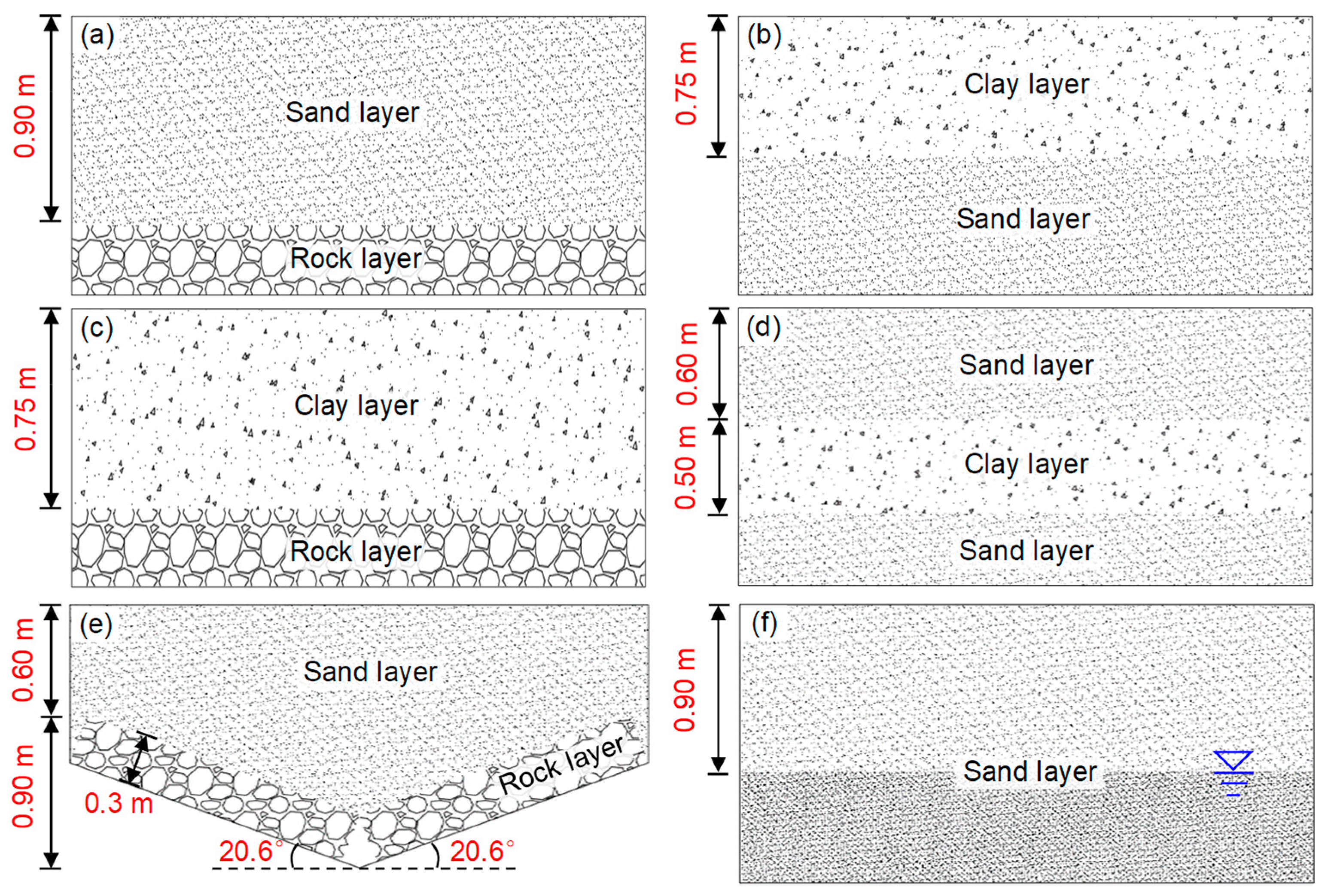
Figure 2.
One trace of reflected waves.

Figure 3.
Ground-penetrating radar equipment.
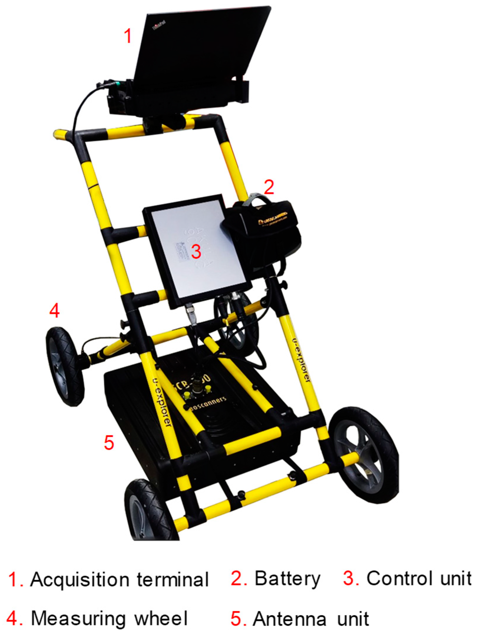
Figure 4.
Horizontal clay–sand model.
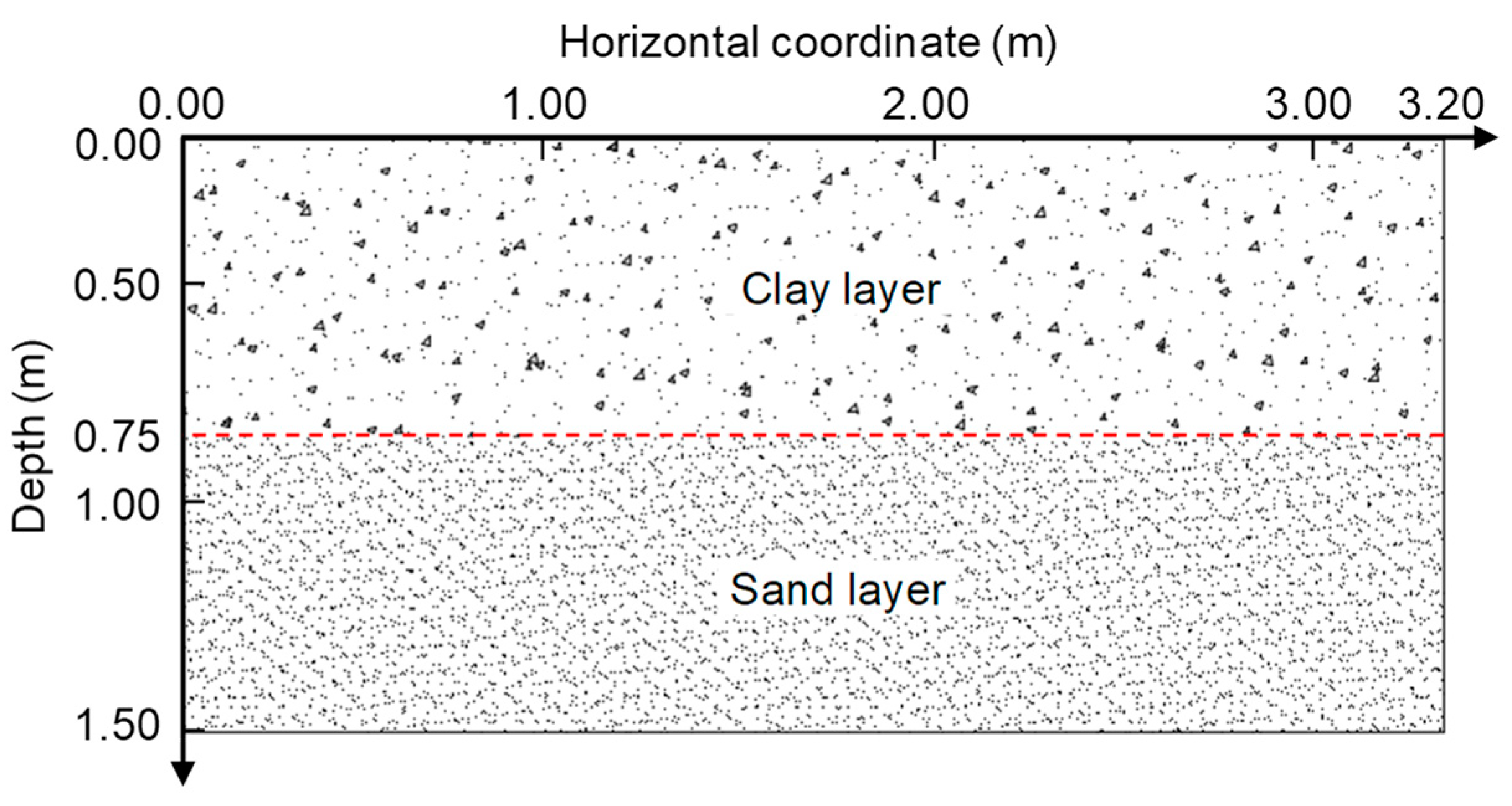
Figure 5.
GPR data of clay–sand model: (a) raw GPR data; and (b) interpreted GPR data.
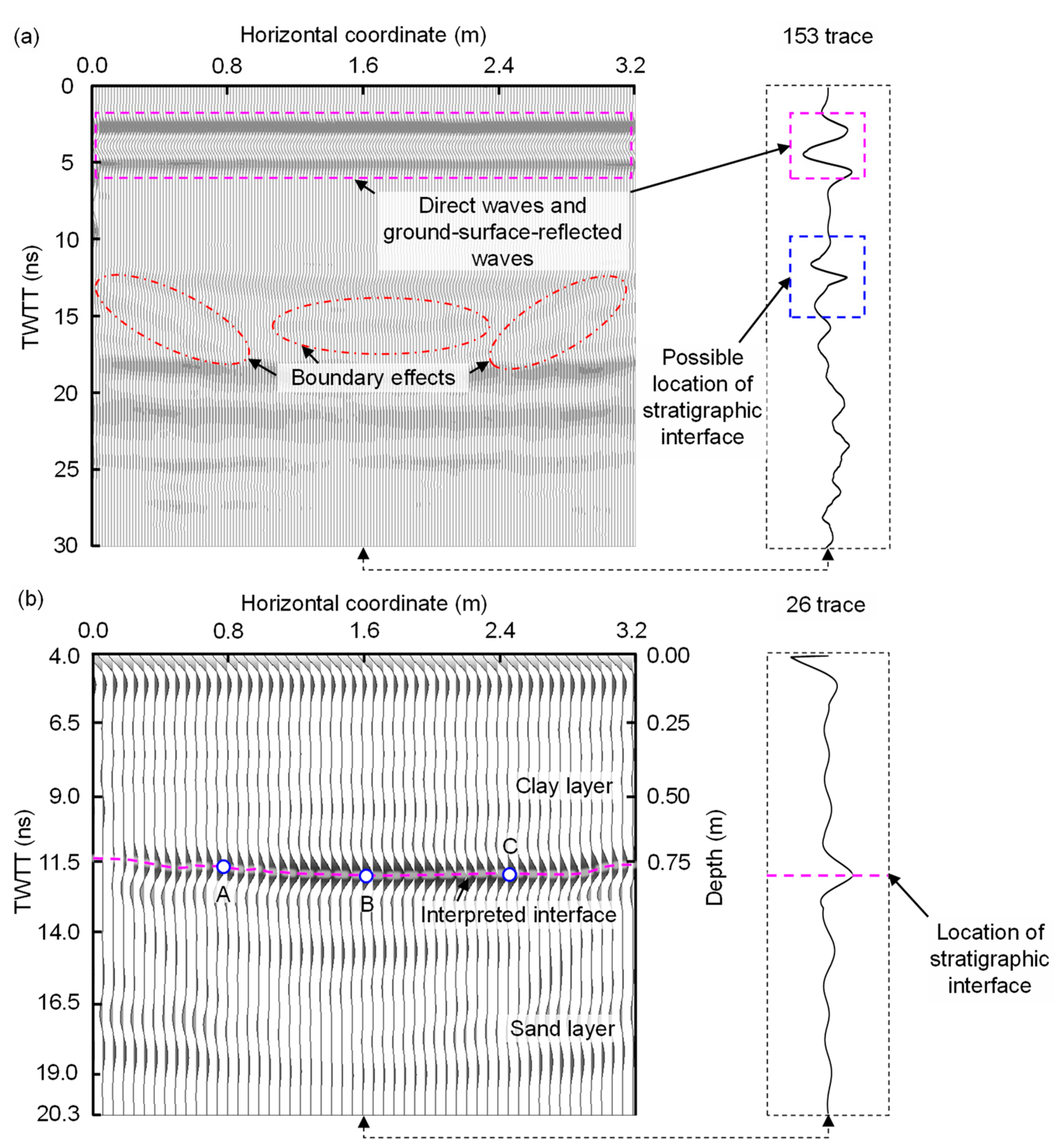
Figure 6.
Absolute and relative errors of clay–sand model: (a) absolute error; and (b) relative error.
Figure 6.
Absolute and relative errors of clay–sand model: (a) absolute error; and (b) relative error.
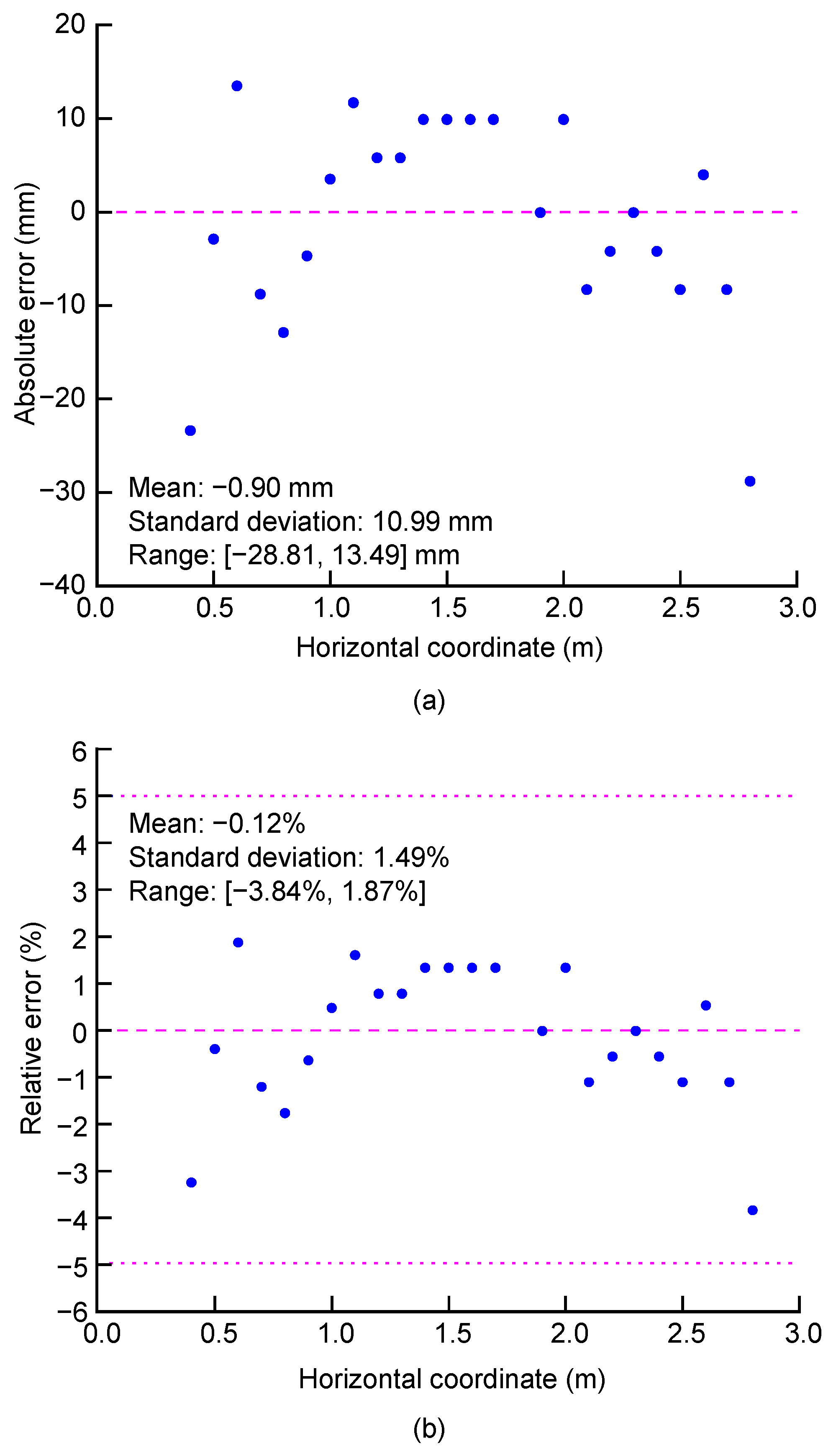
Figure 7.
Physical models and interpreted GPR data: (a) sand–rock model; (b) interpreted GPR data of sand–rock model; (c) clay–rock model; (d) interpreted GPR data of clay–rock model; (e) inclined sand–rock model; (f) interpreted GPR data of inclined sand–rock model; (g) interbedded clay model; (h) interpreted GPR data of interbedded clay model; (i) sand model with a water table; and (j) interpreted GPR data of sand model with a water table.
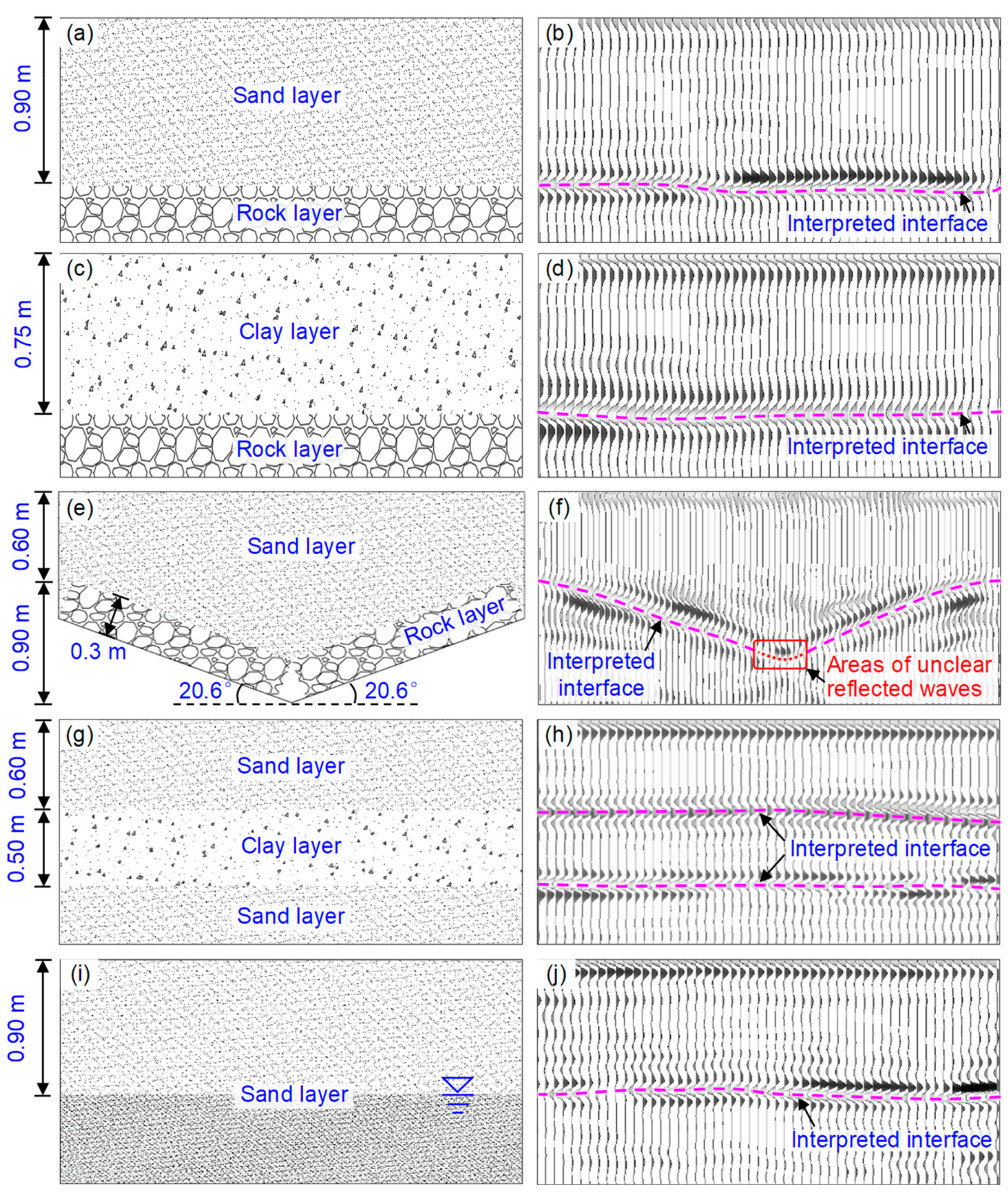
Figure 8.
Relative errors of sand–rock and clay–rock models.
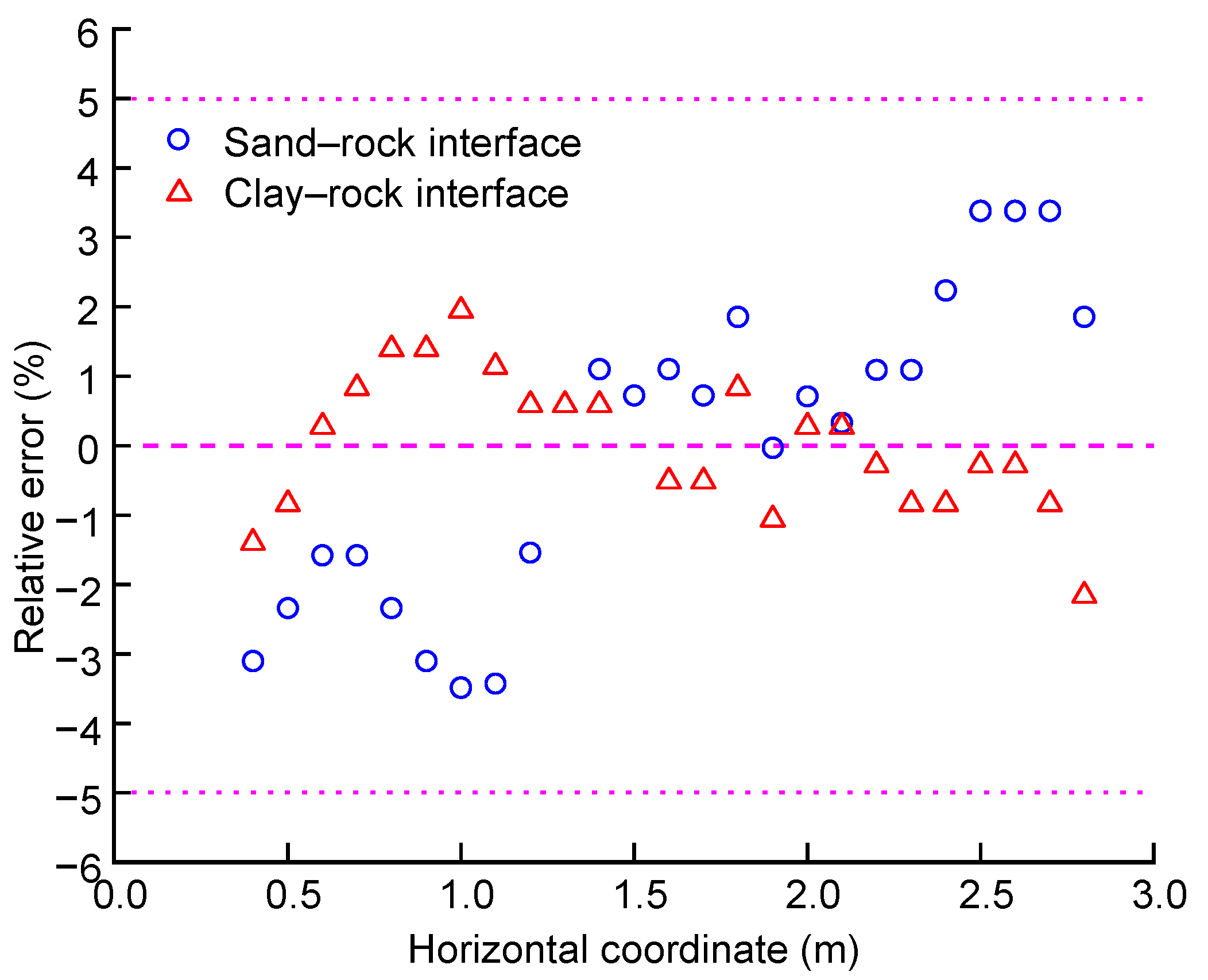
Figure 9.
Measured and interpreted depths of inclined sand–rock model.

Figure 10.
Measured and interpreted depths of interbedded clay model.
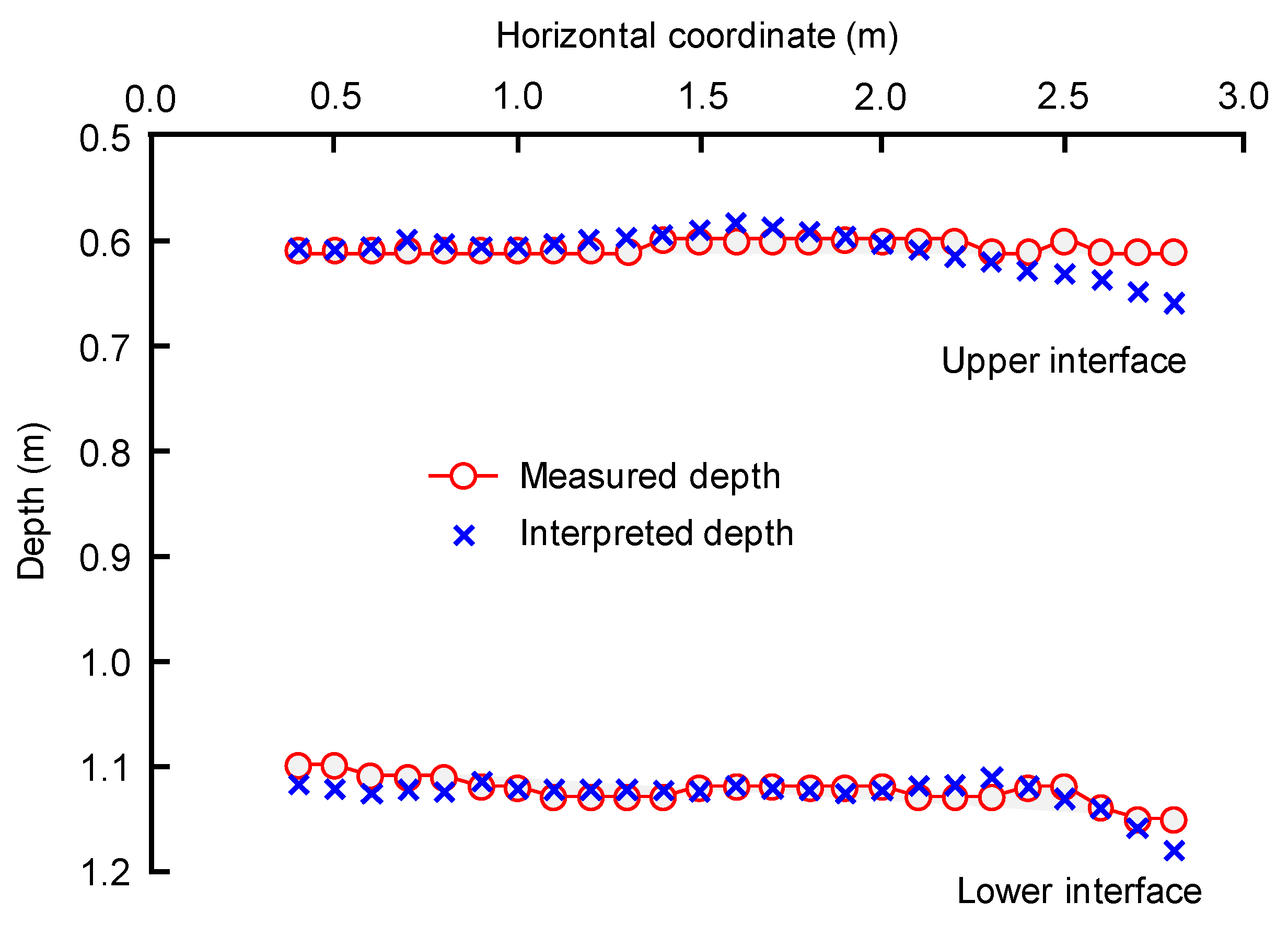
Figure 11.
Relative errors of interbedded clay model.
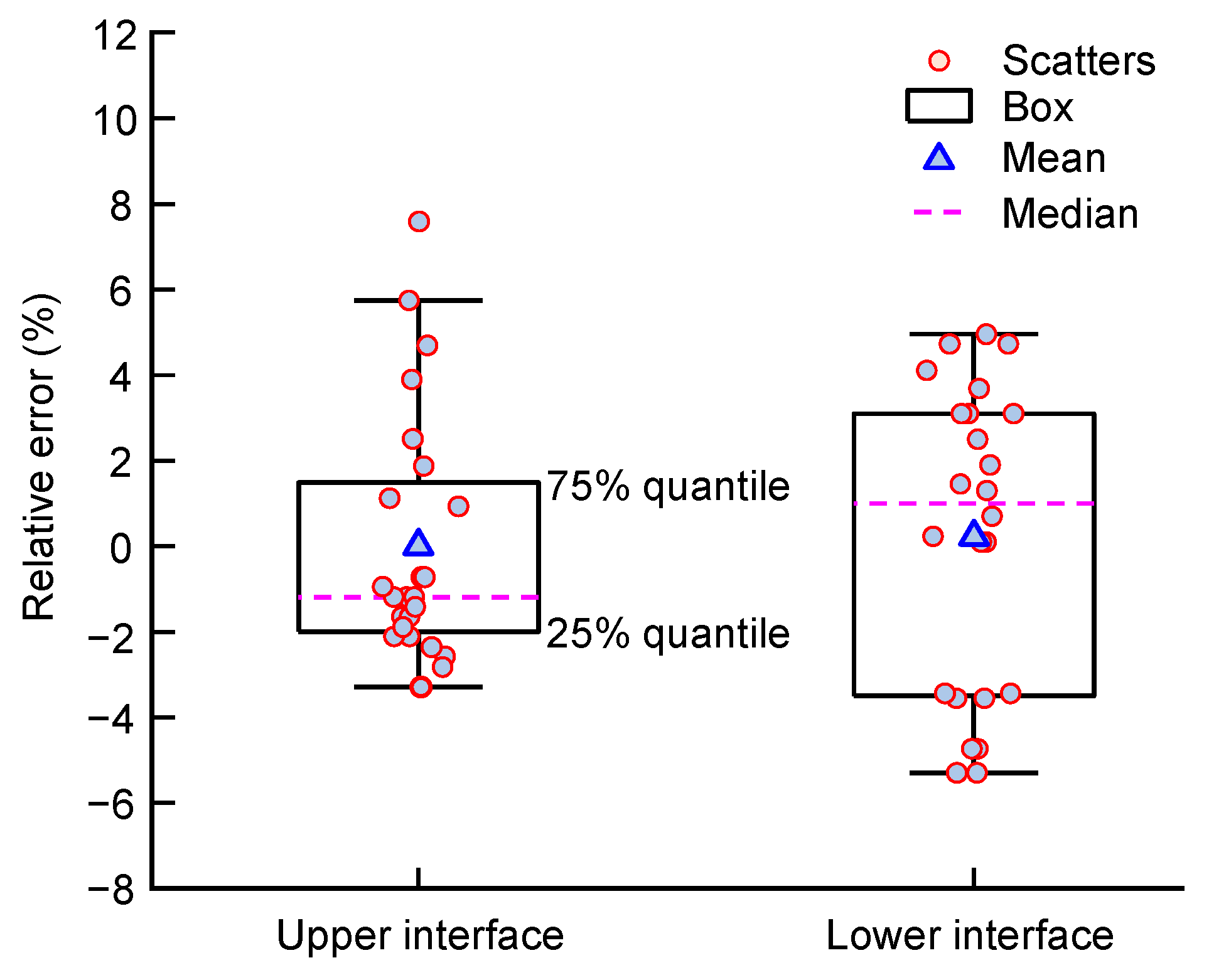
Figure 12.
Relative errors of sand model with a water table.

Figure 13.
Field study of survey profile A–B–C at Tanglang Mountain in China.
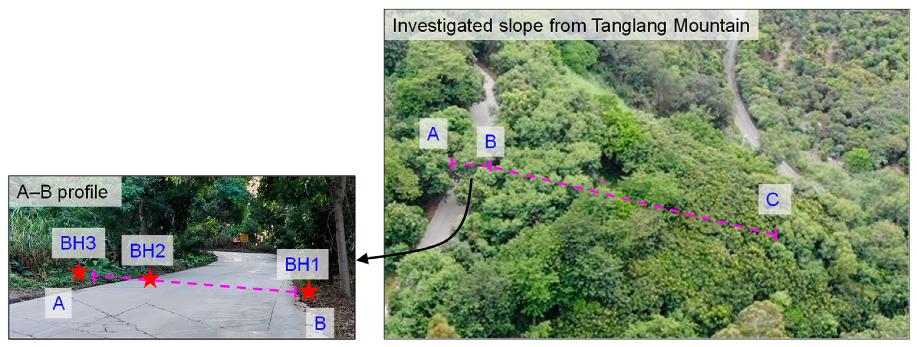
Figure 14.
Interpreted GPR data of survey profile A–B.
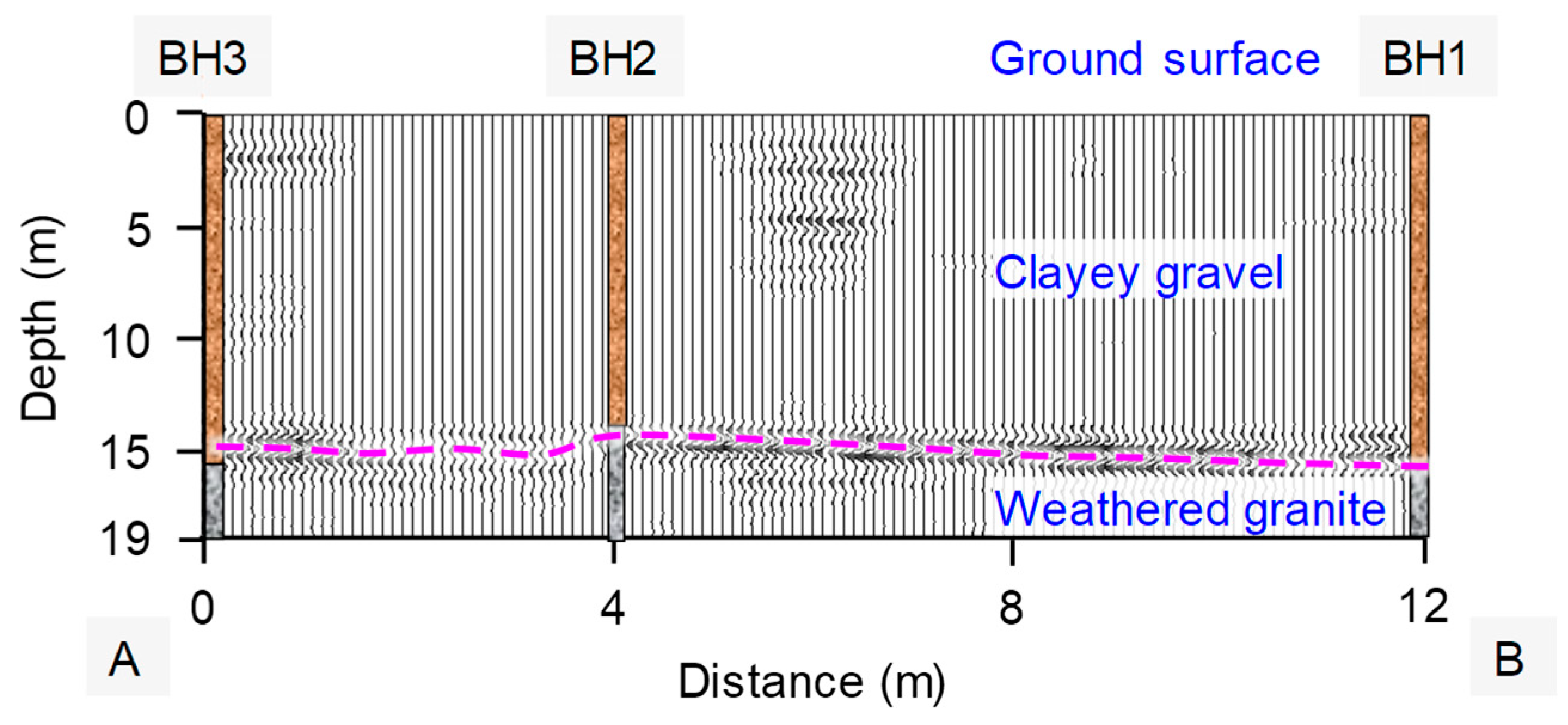
Figure 15.
Interpreted GPR data of survey profile B–C.
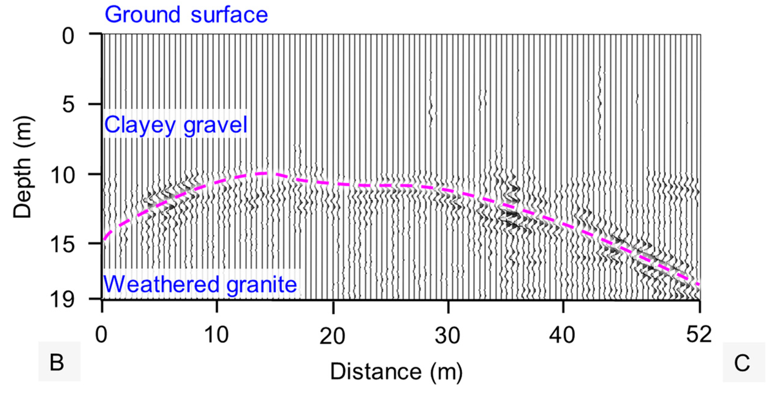
Figure 16.
Geological interpretation of survey profile A–B–C.


Table 1.
Empirical ranges of relative permittivity.
| Material | Range of Relative Permittivity |
|---|---|
| Dry sand | 3–5 |
| Wet sand | 20–30 |
| Limestone | 4–8 |
| Clay | 5–40 |
| Granite | 4–6 |
| Dry salt | 5–6 |
| Shale | 5–15 |
| Silt | 5–30 |
Source: Adapted from Davis and Annan [32].
Disclaimer/Publisher’s Note: The statements, opinions and data contained in all publications are solely those of the individual author(s) and contributor(s) and not of MDPI and/or the editor(s). MDPI and/or the editor(s) disclaim responsibility for any injury to people or property resulting from any ideas, methods, instructions or products referred to in the content. |
© 2024 by the authors. Licensee MDPI, Basel, Switzerland. This article is an open access article distributed under the terms and conditions of the Creative Commons Attribution (CC BY) license (https://creativecommons.org/licenses/by/4.0/).
Share and Cite
MDPI and ACS Style
Wang, T.; Zhang, W.; Li, J.; Liu, D.; Zhang, L. Identification of Complex Slope Subsurface Strata Using Ground-Penetrating Radar. Remote Sens. 2024, 16, 415. https://doi.org/10.3390/rs16020415
AMA Style
Wang T, Zhang W, Li J, Liu D, Zhang L. Identification of Complex Slope Subsurface Strata Using Ground-Penetrating Radar. Remote Sensing. 2024; 16(2):415. https://doi.org/10.3390/rs16020415
Chicago/Turabian StyleWang, Tiancheng, Wensheng Zhang, Jinhui Li, Da Liu, and Limin Zhang. 2024. "Identification of Complex Slope Subsurface Strata Using Ground-Penetrating Radar" Remote Sensing 16, no. 2: 415. https://doi.org/10.3390/rs16020415
Note that from the first issue of 2016, this journal uses article numbers instead of page numbers. See further details here.