Abstract
Wetlands are integral components of agricultural landscapes, providing a wide range of ecological, economic, and social benefits essential for sustainable development and rural livelihoods. Globally, they are vulnerable ecological assets facing several significant threats including water extraction and regulation, land clearing and reclamation, and climate change. Classification and mapping of wetlands in agricultural landscapes is crucial for conserving these ecosystems to maintain their ecological integrity amidst ongoing land-use changes and environmental pressures. This study aims to establish a robust framework for wetland classification and mapping in intensive agricultural landscapes using time series of Sentinel-2 imagery, with a focus on the Gwydir Wetland Complex situated in the northern Murray–Darling Basin—Australia’s largest river system. Using the Google Earth Engine (GEE) platform, we extracted two groups of predictors based on six vegetation indices time series calculated from multi-temporal Sentinel-2 surface reflectance (SR) imagery: the first is statistical features summarizing the time series and the second is phenological features based on harmonic analysis of time series data (HANTS). We developed and evaluated random forest (RF) models for each level of classification with combination of different groups of predictors. Our results show that RF models involving both HANTS and statistical features perform strongly with significantly high overall accuracy and class-weighted F1 scores (p < 0.05) when comparing with models with either statistical or HANTS variables. While the models have excellent performance (F-score greater than 0.9) in distinguishing wetlands from other landcovers (croplands, terrestrial uplands, and open waters), the inter-class discriminating power among wetlands is class-specific: wetlands that are frequently inundated (including river red gum forests and wetlands dominated by common reed, water couch, and marsh club-rush) are generally better identified than the ones that are flooded less frequently, such as sedgelands and woodlands dominated by black box and coolabah. This study demonstrates that HANTS features extracted from time series Sentinel data can significantly improve the accuracy of wetland mapping in highly fragmentated agricultural landscapes. Thus, this framework enables wetland classification and mapping to be updated on a regular basis to better understand the dynamic nature of these complex ecosystems and improve long-term wetland monitoring.
1. Introduction
Floodplain wetlands in arid and semi-arid regions are formed by and respond to the periodic flooding of adjacent rivers [1,2,3]. They are dynamic ecosystems that contribute significantly to regional hydrological and ecological functions [4,5], and provide a range of ecological services [6] such as biodiversity conservation [7], water quality improvement [8], and carbon sequestration [9]. In intensive agricultural landscapes, these ecosystems are critical for regional ecological health [10,11]. Floodplain wetlands support rich biodiversity: their presence increases landscape complexity within a terrestrial mosaic. They provide habitat and forage for breeding waterbirds and offer refugia for a wide range of invertebrate wildlife, including many that are agriculturally beneficial such as pollinators and natural pest predators [12].
Despite their resilience and adaptability [13], these unique ecosystems are increasingly under threat from climate change and human activities such as the expansion of agriculture and associated irrigation, extensive water resource development, including dam construction and water diversion, and infrastructure development [14,15]. The loss of these floodplain wetlands can have devastating impacts on local biodiversity and the overall health of the semi-arid landscapes [16]. To prevent further losses and degradation of these critical ecosystems, effective management strategies are required.
Mapping is an indispensable tool for effective wetland monitoring and conservation. It guides management decisions, and facilitates adaptive management [17,18], especially in the context of the increasing unpredictability of climatic patterns associated with climate change [19,20]. Mapping wetlands using traditional methods, such as ground survey and aerial photo interpretation, is often time-consuming and resource-intensive [21]. Machine learning algorithms, coupled with satellite imagery, offer promising solutions for automated and accurate wetland mapping [22,23,24], providing essential insights into their dynamics and responses to environmental changes [25,26]. Many studies have demonstrated the efficiency and accuracy of wetland mapping at regional, national, and global scales by applying machine learning algorithms to satellite data [21]. Using random forest (RF) with Landsat-8 data, Amani et al. [27] presents the first Canadian national wetland inventory, with an overall accuracy of 70.6%. Aiming to improve accuracy and efficiency in wetland mapping, LaRocque et al. [28] employed various classification techniques to delineate 11 wetland classes in southern New Brunswick, Canada. By utilizing a combination of remote sensing data sources including Landsat 8 OLI, Sentinel-1, ALOS-1 PALSAR, and LiDAR, they were able to achieve an overall accuracy of 97.67%. Li et al. [29] also proposed an approach that integrated spectral indices derived from Landsat and Sentinel satellite imagery, topographic variables, and climatic data within the GEE platform to classify wetlands for the entire continent of Africa while achieving promising results.
Wetland mapping in intensive agricultural landscapes presents several unique challenges due to the dynamic nature of these ecosystems and the interactions with human activities. First, agricultural landscapes are characterized by diverse land uses and management practices, leading to high variations in wetland types and characteristics over a relatively small space [30]. This heterogeneity makes it difficult to develop standardized mapping approaches. Second, wetlands can vary in size and shape, ranging from small, isolated patches to large complexes [31] or narrow linear features fringing the riparian zones [32], requiring high-resolution data and sophisticated analytical techniques. Third, wetlands in agricultural landscapes are subject to more frequent temporal changes due to seasonal fluctuations, land-use changes (e.g., crop rotation), and management practices, such as irrigation and drainage. Mapping efforts need to account for these dynamics to achieve a satisfactory performance. Finally, vegetation cover in agricultural landscapes can obscure wetland boundaries. For example, the optical signatures between irrigated crops and flooded amphibious plants can be barely distinguishable, resulting in less-than-optimal classification and mapping accuracy in comparing with other landcover types [33]. Discriminating between wetland vegetation and surrounding landcover types requires advanced remote sensing techniques, such as hyperspectral imagery [34], which are not publicly available and limited to small geographic areas. Recent studies [35,36] demonstrate the potential of multi-temporal imagery that highlights plant phenological differences in species-based vegetation community classification, leading to the introduction of land surface phenological metrics in wetland classification and mapping [37]. A variety of methods have been applied to multi-temporal spatial data to extract phenological metrics (see a recent review by Misra et al. [38]). The harmonic analysis of time series (HANTS) algorithm, introduced by Verhoef [39] for the reconstruction of outliers and missing data simultaneously in time series with periodic behaviour, is more suitable for natural vegetation, such as forests, shrublands, and perennial grasslands, which might experience limited multi-annual variation [40]. By integrating phenological variables derived from time series of remote sensing data, researchers can improve the classification and mapping of wetland types, providing valuable insights for wetland management, conservation, and monitoring efforts [35,41,42]. This approach utilizes remote sensing imagery collected over a period (normally over a year) to extract phenological variables that can capture the unique vegetation response to the changes in environmental conditions (e.g., water availability and soil moisture) and inundation regimes associated with specific wetland vegetation types [42].
This study aims to establish a robust framework for wetland classification and mapping in intensive agricultural landscapes using time series of Sentinel-2 imagery, with a focus on the Gwydir Wetland Complex. The wetlands are located in the northern Murray–Darling Basin—Australia’s largest system of interconnected rivers. Despite being extensively affected by long-term agricultural expansion, the Gwydir Wetland Complex remains notable for its ecological significance and rich biodiversity, encompassing a diverse array of wetland types such as floodplain marshes, woodlands, and riparian open forests, [43,44]. Specifically, the study seeks to (1) evaluate the contribution of HANTS metrics to wetland mapping by comparing models with and without them, and (2) assess the performance of random forest algorithms in discriminating compositional wetland vegetation types with similar ecohydrological settings using the most effective predictors.
2. Methods
2.1. Study Area
The Gwydir Wetland Complex (Figure 1) is a significant wetland system located in the northern part of New South Wales, Australia. It includes floodplain wetlands lakes and river channels and covers approximately 200,000 hectares. This wetland complex that includes two internationally recognized Ramsar sites and is renowned for its ecological importance, providing critical habitat for a wide variety of flora and fauna, including numerous species of waterbirds, fish, and reptiles [44]. The Gwydir Wetland Complex is also recognized for its cultural significance to Indigenous communities, who have long-standing connections to the land and waterways within the region [45].
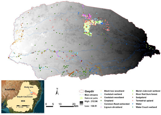
Figure 1.
The distribution of field sampling plots in the Gwydir Wetland Complex, located downstream of Gwydir catchment in the Murray–Darling Basin of Australia (inset map).
Despite its ecological and cultural significance, the Gwydir Wetland Complex faces multiple threats. These include habitat degradation due to human activities such as water extraction for agriculture, invasive species, and altered flow regimes. The landscape of the Gwydir Wetland Complex is marked by a mosaic of water regimes ranging from permanent to ephemeral wetlands, which are interspersed with agricultural lands. The wetlands themselves are often described as relic wetlands, highlighting their reduced and fragmented state due to historical land-use changes and water management practices. These relic wetlands typically manifest as small, fragmented, and linear features along streams, reflecting the impact of agricultural expansion and water diversion for irrigation. Conservation efforts, such as providing environmental water for key vegetation communities (e.g., Bolboschoenus wetlands), are a major management action to protect and restore this valuable ecosystem.
2.2. Field Survey
Ground-based surveys are crucial for calibrating and validating wetland mapping based on remote sensing data. On-ground surveys enabled the validation and identification of wetland boundaries, vegetation types, and hydrological characteristics. To ensure our plots covered all major vegetation types, we adopted a stratified random sampling approach to create field survey points. Firstly, we stratified the study area using three information layers: vegetation class (nine vegetation classes mapped in 2015), preferred inundation frequency following Roberts and Marston [46], and soil landscapes [47]. We rasterised the shapefiles of these three information layers, stacked them, and created a 100 m internal buffer from the boundaries of National Parks and Crownlands and a 50m internal buffer for accessible roadside areas. This step divided the study area into relatively homogeneous units (i.e., strata) in terms of vegetation composition. As the relic natural vegetation areas in private lands are normally irregular and small, the grids size was 150 m × 150 m (vs. 250 m × 250 m in National Parks and Crownland areas) to ensure enough sample sites. A total of 730 random sample sites were then drawn from the strata.
In June and July 2023, we collected rapid floristic data from 445 of the 730 randomly generated points due to restricted access in some areas of the Gwydir Wetlands. We recorded the identity and percentage cover of the five most dominant species in each stratum within a 20 m × 20 m randomly generated plot, as well as its environmental attributes (landscape position and soil characteristics).
To supplement our ground data in areas with limited access, ground data points were utilized from contemporary mapping exercises within the study area. This included an additional 326 ground data points from systematic and random meander vegetation points [48], and by a consultancy team (the Alluvium Group (Eco Futures)) who provided unpublished vegetation survey data as part of their preliminary mapping study of the vegetation of the Mallowa creek region. Since the vegetation survey schemes were the same, we combined the two datasets to map the wetlands for the entire study area.
2.3. Vegetation Compositional Types
Each of the 771 ground survey samples was assigned a plant community type (PCT), which is the master community-level typology used in New South Wales (NSW) planning and assessment tools and state vegetation mapping and management programs (NSW BioNet, website visit on 28 April 2024: https://www.environment.nsw.gov.au/topics/animals-and-plants/biodiversity/nsw-bionet/about-bionet-vegetation-classification). We then aggregated the PCTs into three levels of classification (Table 1). The first level distinguishes wetlands from other landcover types, i.e., croplands including irrigated pastures, surface water—mainly farm dams, and terrestrial upland in more or less natural condition. The second level further divides wetlands into five functional groups: the frequently flooded river red gum (Eucalyptus camaldulensis) forest, woodland, shrubland dominated by shrub species including lignum (Duma florulenta) and nitre goosefoot (Chenopodium nitrariaceum) and small trees such as river cooba (Acacia stenophylla), sedgeland—the intermittent grass-dominated wetlands, and marshes—frequently inundated wetlands dominated by aquatic plant species. The third level distinguishes three woodlands: coolibah (Eucalyptus coolabah) wetland dominated by coolibah and river cooba (Acacia stenophylla), coolibah woodland (dominated by E. coolabah) and black box (E. largiflorens) woodland; and three marshes based on dominant species: common reed or cumbungi (Phragmites australis and Typha spp.) wetland, water couch (Paspalum distichum) wetland, and marsh club-rush (Bolboschoenus fluviatilis) wetland. The second and third level classification were based on the NSW plant community types. We did not separate other landcover types into more detailed classes since the focus of this study was to improve the performance of wetland mapping.

Table 1.
The three levels landcover samples in the Gwydir Wetland Complex.
We developed three sets of machine learning classification models for each level of landcover (see Section 2.6 below) that resulted in a total of nine landcover maps. We then compared the performance of the nine models using a benchmark experiment [48,49] approach. This enables maps with different levels of detail to be used for specific management purposes. For example, level one maps could be used for environmental reporting, while level three maps could be used to guide environmental water delivery to a targeted wetland community.
2.4. Topographic Variables
We downloaded the 5 m airborne light detection and ranging (LiDAR) digital elevation model (DEM) covering the study site from Geoscience Australia (https://elevation.fsdf.org.au/, website accessed on 15 February 2024). The 5 m DEM was corrected with field survey transects for streams and water bodies using field survey transects; it has a fundamental vertical accuracy of at least 0.30 m (95% confidence) and horizontal accuracy of at least 0.80 m (95% confidence). The 5 m DEM was resampled to 20 m using bilinear interpolation. The detailed LiDAR DEM is not available for the western part of the Gwydir Catchment. The gap was filled with the 30 m smoothed digital elevation model (DEM-S) using a simple linear regression. DEM-S was derived from the SRTM data acquired by NASA in February 2000 [50]. DEM-S represents ground surface topography (excluding vegetation features) and has been smoothed to reduce noise and improve the representation of surface shape [51]. Three topographic variables were derived from the DEM-S: de-trended DEM, local (within a 3 × 3 pixel window) deviation from global, and surface curvature, which is the second derivative of a surface (i.e., the slope of the slope) [52,53,54]. The three variables are all related to water availability and soil moisture condition, which are important for vegetation establishment and growth.
2.5. Sentinel-2 Based Variables
All available Sentinel-2 atmospheric corrected surface reflectance (SR) images (a total of 152 from two tiles) for the 2022 water year (30 June 2022–1 July 2023) were used for landcover classification and mapping. Sentinel-2 Earth observation mission by the European Space Agency consists of two satellites (Sentinel-2A and Sentinel-2B) with a revisit frequency of 5 days. Image pre-processing (including cloud and cloud shadow masking), calculating vegetation indices (VI) and statistical summary of VI time series, and phenological feature extracting, were conducted using the Google Earth Engine (GEE) platform. The cloud and cloud shadow were masked out at pixel level with the Cloud Score+ S2_HARMONIZED dataset [55]. We adopted a relatively high-quality score (0.70) to remove the occluded pixels.
2.5.1. Tasseled Cap Transformations (TCT)
Previous studies [56,57,58] have shown that Tasseled Cap transformations (TCT) [57] can be valuable in remote sensing classification by reducing dimensionality, extracting relevant features, enhancing discrimination, and reducing noise. By integrating TCT with classification techniques, valuable thematic information from remote sensing imagery can be extracted for various applications, including landcover mapping, land-use classification, and environmental monitoring. In this study, three TCT components, for brightness, wetness, and greenness, were calculated from the median image of the time series using the coefficients proposed by Healey et al. [58].
2.5.2. Vegetation Indices and Calculation of Statistical and Phenological Features
There are more than 100 empirical spectral-based vegetation indices (VI) being developed and used to monitor Earth system dynamics [59,60]. We selected six VIs derived from multispectral Sentinel-2 SR imagery to suit cropland dominance in the landscape: the generalized kernel NDVI (kNDVI), the inverted red-edge chlorophyll index (IRECI), the modified normalized difference water index (MNDWI), the normalized difference moisture index (NDMI), and the enhanced modified bare soil index (EMBI) (Table 2).
Table 2.
Spectral indices used to discriminate landcover in the Gwydir Wetland Complex.
Using the time series of VI, two groups of predictor variables were calculated to develop machine learning classification models: statistical and phenological features.
The statistical features are the five simple summary variables, including minimum, median, maximum, the range average in the 25–75% percentile intervals, and standard deviation of the six vegetation indices.
The phenological features are based on the harmonic analysis of time series data (HANTS). HANTS is one of the most widely recognized reconstruction methods to model satellite time series observations [67]. HANTS decomposes time series into a series of harmonic components (i.e., a set of sine or cosine curves in Equation (1)), which capture the seasonal variation, periodic trends, and cyclic patterns present in the remote sensing data [68].
Different landcover types, such as forests, croplands, and water bodies, exhibit distinct temporal patterns in terms of vegetation growth, phenology, and land surface dynamics [68,69]. By analysing the harmonic components of time series remote sensing data, landcover types can be effectively discriminated and classified with high accuracy [68]. Here, we explored the potential of the extracted phenological metrics (i.e., the amplitude (Equation (2)) and phase (Equation (3)) of all harmonic components) to further distinguish the wetland vegetation communities (Table 2).
where is the fitted value at date t; T is mean number of days in a year (i.e., T = 365.2425); and N is the number of cycles in the time series (i.e., the number of harmonic components associated with the frequency of the time series, T). The harmonics (we selected two in this study) consist of a base frequency and a series of integer multiples of the base frequency; an and bn are coefficients of the trigonometric components; a0 can be viewed as the coefficient at zero frequency, which is the average of the series; c is the linear trend; and is the residual of harmonic fitting.
With the fitted coefficients, amplitude and phase for the n-th harmonic components are calculated:
The model residuals, amplitude, and phase for both harmonic components were used as HANTS features for the development of classification models. We included the residuals to capture the possible erratic response of riparian vegetation communities to river flows, which may not manifest in broad floodplain communities.
All predictors were resampled to 20m spatial resolution for consistency.
2.6. Machine Learning Classification
2.6.1. Development of Random Forest Models
We modelled the distribution of the landcover classes using random forest (RF) implemented in the R package “Caret” [70]. RF is an extension of decision tree classifiers, consisting of an ensemble of decision trees, in which each tree is constructed using a subset of training samples with replacements [71]. RF is a widely used supervised machine learning method for classification and regression [72], especially for landcover and land-use mapping. It is also useful in discriminating wetland vegetation compositions [73,74].
We developed three set random forest (RF) models (Table 3) for each level of landcover classification. The most comprehensive models have all the predictors, i.e., topographic and TCT (inferred as basic predictors thereafter) and both statistical and HANTS features. The others involved basic predictors, and either statistically or HANTS-generated features.
Table 3.
Inputs for random forest classifiers.
Before modelling, all predictor variables are normalized so that the whole dataset is in a common frame [75]. The dataset was split into training (75%) and testing (25%) subsets using stratified random sampling. With the training dataset, a 10-fold repeated (5 times) cross-validation method was used for model tuning. The landcover (use) classes are highly unbalanced (minimum 17 and maximum 130, Table 1), and most machine learning models tend to be more efficient and accurate in predicting the majority class than the minority class [76]. In model tuning, we adopted the hybrid “smote” (synthetic minority sampling technique), which down samples the majority class and synthesizes new minority instances by interpolating between existing ones [77] to correct this behaviour, so that class frequencies match the least prevalent class. The “smote” was conducted inside of resampling when calling the “train” function of “Caret” package. In addition, we determined the “granularity” of the tune grid by setting the tuneLength = 10 in the “train” function to search the optimal model that has the highest accuracy.
Although RF is relatively robust to correlated predictor variables [78], highly correlated inputs could lead to inflated training performance and lower the prediction power [79]. To identify and exclude highly correlated predictors, we first randomly sampled 5000 points from the model domain (i.e., the entire Gwydir Wetland Complex), and used the 5000 points to extract all predictor variables. We then used variance inflation factor (VIF) to test the collinearity among variables. Variables with a VIF greater than 5 [79] were excluded for the following modelling.
2.6.2. Classification Accuracy
The classification accuracy was assessed at both model and class level. At model level, we evaluated the performance with two widely used metrics in machine learning: the overall accuracy (OA, Equation (4)) and sample-weighted F1 score (Equation (6)). Both metrics have their own advantages and disadvantages. With the F1 score, the harmonic mean of the precision and recall of a classification model (Equation (5)) offers a more nuanced evaluation; however, overall accuracy provides a straightforward measure of correctness. The choice between the two depends on the specific requirements of the classification problem and the class distribution of the dataset [80].
At class level, the class-dependent performance of fitted models in separating one landcover from others was evaluated in terms of F1 score, precision (Equation (7)) and recall (Equation (8)). We report both training and testing performance metrics. The overall accuracy, precision, recall, and F1 score (Equation (5)) were calculated from the confusion matrix.
where TN and TP are true negative and true positive; and FN and FP are false negative and false positive, respectively. N is the number of total samples and ni is the number of samples for class i.
Please note that the model tuning includes a 10-fold cross-validation procedure, which splits the training dataset into 75/25 for model checking. Therefore, the difference between the training and testing accuracy should be minimal if there are sufficient samples.
2.7. Model Comparison
A benchmark experiment [46,47] was adopted to compare the performance of the three sets of RF models for each classification level. In benchmarking, 50 samples are drawn from the same training dataset (by setting the same seed number during model tuning) using bootstrapping, i.e., resampling with replacement. The significance in difference of model performance metrics (we included overall accuracy and the means of precision, recall and F1-score across the classes) was then tested using a simple t-test with Bonferroni-adjusted p value.
3. Results
3.1. Model Performance
3.1.1. Level One Classification
All models performed well for level one classification according to the weighted F1 score and overall accuracy (Table 4). Moreover, the performance of testing is comparable to that of training, indicating there is limited concern of overfitting [81].
Table 4.
Performance of Level 1 classification models for the Gwydir Wetland Complex.
For each landcover class, the models were excellent for separating wetlands and croplands from other classes (i.e., all training F1 scores are greater than 0.9 and the overall accuracy was greater than or close to 0.9). The worst case was for discriminating terrestrial from other classes with training F1 scores of 0.706, 0.634, and 0.692 for M1, M2, and M3, respectively. However, the classification may be considered efficient even for the worst case (i.e., F1 score > 0.6). For open water, the training performance was good (F1 score > 0.8); however, there was a large decrease in the testing performance (F1 score = 0.667 for all models). The discrepancy is likely caused by the small test samples. With only four testing samples, one error resulted in dramatic reductions in performance assessment metrics.
3.1.2. Level Two Classification
Further discrimination of wetlands into five broad groups decreased the models’ performance (Table 5). Generally, the weighted F1 score and overall accuracy were greater than 0.7, meaning these models were considered sufficient.
Table 5.
Performance of Level 2 classification models for the Gwydir Wetland Complex.
For the modelled wetland classes, the classifiers were highly efficient in detecting marshes, especially with features including phenology (i.e., M1 and M3) (F1 score > 0.8, Table 5). Moreover, the comparable precision and recall indicated that the models were well-balanced. They had high capacity to correctly identify marshes and to avoid wrongly classifying other vegetation communities as marshes. In contrast, the models were less efficient in discriminating shrub wetlands even with all predictors (F1 score = 0.608 and 0.744 for training and testing datasets, respectively, Table 5). A close examination of the confusion matrix revealed that the inter-class misinterpretations between woodlands and shrublands contributed the most to the low discrimination power. Nevertheless, the F1 score suggested a good classification (F1 = 0.797 and 0.744 for M1 training and testing Table 5) for woodlands, and the precision and recall indicated that the model was well-balanced. The inconsistency is likely due to the imbalance in the sample number (the woodland has nearly three times more samples than shrubland). The models were also sufficient in identifying river red gum forests. However, the lower precision suggested that the models tended to mis-classify other landcover types as river red gum forests (shrublands and woodlands based on the model confusion matrix).
3.1.3. Level Three Classification
When progressing to separate the wetlands into more detailed groups with different vegetation compositions, the model performance metrics deteriorated as expected (Table 6). However, the models were still useful with the overall accuracy and F1 score close to 0.7, especially for M1. In comparison with the woodlands, the models were more efficient at discriminating the vegetation communities within the more frequently flooded marshes.
Table 6.
Performance of Level 3 classification models for the Gwydir Wetland Complex.
Wetlands dominated by water couch were classified with very high precision and recall (greater than 0.9, Table 6), followed by those dominated by marsh club-rush (F1 score = 0.775). Even though the F1 score was lower for the common reed wetlands and sedgelands, it was still greater than 0.5, and the models can be considered acceptable. While the confusion with woodlands contributed the most to the low performance for sedgelands, the low F1 score for the common reed wetland was mostly caused by the confusion with sedgelands.
3.2. Model Comparison
For the three levels of classification, the model with all predictors (M1) had significantly better performances in the majority of cases in terms of F1 score, overall accuracy, and mean recall and precision (Table 7, Figure 2). The performance difference between M1 and M2 (model with basic predictors and statistical features) was higher than that between M1 and M3 (model with basic predictors and HANTS features). Although M3 generally had better performance than M2, the difference was not significant in some cases (Table 7).
Table 7.
The difference in performance metrices between models (p values in bold indicate the difference is significant at 0.05 level) for the Gwydir Wetland Complex.
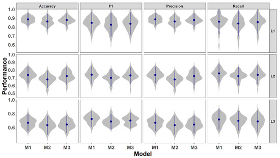
Figure 2.
The distribution of model performance metrics generated by resampling the predictions using the same testing dataset. Dots are the mean, vertical bars are the standard deviation, and shadows are the distribution of the 50 resamples. M1 = model with all predictors; M2 = model with basic predictors and statistical features; and M3 = model with basic predictors and HANTS features. L1, L2, and L3 are class level 1 (4 types), level 2 (8 types), and level 3 (12 types).
For all performance metrics of the three levels of classification, M1 had the smallest standard deviation (sd, Figure 2), suggesting that the models with all predictor variables were the most balanced and robust; therefore, prediction maps produced with M1 would have highest reliability.
3.3. Predicted Wetland Distribution
Figure 3 presents the nine prediction maps. We did not have access to contemporary, independent landcover maps for comparison, so we have used aerial photos captured in 2022 for qualitative comparison purposes (Figure 4). We focused on the prediction of M1, the most robust classifier.
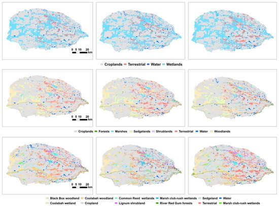
Figure 3.
Predicted landcover/land-use maps from level 1 (upper), 2 (middle), and 3 (lower) classification with M1 (left), M2 (middle), and M3 (right).
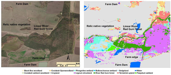
Figure 4.
Virtual comparison between aerial photo and predicted landcover types of a section in Gwydir Wetland System showing the correct identification of small farm dams, relic native vegetation patches, and linear river red gum forests along creeks.
The largest landcover in the Gwydir is cropland, and accounts for more than 60% of the total modelled domain (276,005 ha, Table 8), followed by wetlands (126,178 ha or 29.05%), terrestrial vegetation (21,622 ha, 4.98%), and open water (10,511 ha, 2.42%). Note that the mapped croplands were cultivated lands, as the edges of paddies, often covered by shrubs and grasses, were generally modelled as shrublands (Figure 4).
Table 8.
Summary of the mapped landcover in Gwydir based on the prediction maps of M1 that involved all predictor variables.
The model is highly efficient in delineation of surface waters, most of which are farm dams for irrigation. M1 correctly identified all 91 mapped farm dams in the 2017 land-use map [82], and the smallest dam identified using M1 has an area of just over 3000 m2 (8 modelling pixels).
The mapped river red gum forests, which are linear features along the main rivers and streams, were largely in agreement with the aerial photos (Figure 4). The total area of river red gum forests was 5775 ha (1.33%).
Small patches of relic natural landcover (wetlands and terrestrial vegetation) within the croplands were also correctly identified and delineated (Figure 4).
3.4. Key Predictors to Discriminate Wetland
The VIF process selected a total of 34 predictor variables to build the random forest model. Predictors from all four groups were selected (Figure 5). Also, features (simple statistics and/or HANTS) from all six vegetation indices were involved. One topographic variable (detrended elevation) and one TCT component (brightness) were included in the modelling procedure. The spatial and temporal variations of the other two TCT components, i.e., greenness and wetness, are likely captioned by vegetation indices such as MNDWI and NDMI. The most important variable was the mean MNDWI, followed by minimum NDRE.
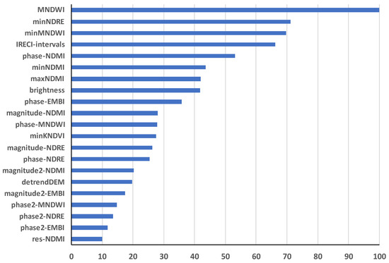
Figure 5.
Importance of the top 21 predictors with importance of over 10. Importance is scored so the most important variable has a score of 100, and the variable with least contribution to the performance of the model has a score of 0. Res-NDMI is the residuals of the harmonical fitting of NDMI time series.
4. Discussion
Our study found that land surface phenological metrics are important in discriminating relic wetlands in highly fragmented agricultural landscapes. Furthermore, we showed the potential and limitations of using machine learning algorithms with phenological variables for delineation of wetlands with different vegetation compositions.
4.1. The Value of HANTS in Wetland Identification
The RF models that included HANTS features generally had better performance for all three levels of classification (i.e., higher overall accuracy and weighted F1 score, Table 4, Table 5 and Table 6), and the difference was significant in almost all cases according to the analysis of the benchmark experiments (Table 7). The findings suggest that harmonic analysis of satellite time series is a powerful technique for landcover classification and mapping [67], especially for differentiating wetlands with different vegetation composition [38].
Different landcover classes may exhibit distinct seasonal patterns of growth, phenology, and reflectance due to varying environmental factors and land management practices [83]. Harmonic analysis effectively captures these temporal signatures, enabling the identification and characterization of different landcover types based on their unique temporal behaviour (Figure S1). The simple statistical summary of the VI time series, such as the annual medium, minimum, maximum, and standard deviation, focuses on the prevailing conditions and may not reflect the finer temporal dynamics. Many studies recognized the importance of seasonal patterns of growth and used seasonal summary of remote sensing data for vegetation classification and mapping [3,35]. The inclusion of HANTS features (i.e., amplitude and phases in this study) facilitates the detection of subtle variations and trends that may not be apparent from statistical features. The comparison between M2 and M3 (Table 7) demonstrates the superiority of HANTS features over statistical features in differentiating landcover types.
4.2. The Potential and Limits of Using HANTS Features to Discriminate Wetland Types
The study also demonstrates the potentials of HANTS features in differentiating the major wetland types with different vegetation communities. Our results show that the RF models with all predictors can separate wetland types based on the vegetation compositions with high accuracy for the low-laying and frequently flooded river red gum forests and grassy marshes. These wetlands are relatively homogeneous in terms of vegetation composition. For example, the marsh club-rush wetland is dominated by Bolboschoenus fluviatilis (canopy cover generally > 40%), which forms densely, and stands up to 2 m tall [84]. Nevertheless, the inter-class confusion (Table S1) increased when vegetation cover became more heterogeneous within transition zones. For example, the models had the lowest performance for sedgelands, which are often found between the edge of (semi-)permanent marshes and terrestrial uplands, typically consisting of wetland plants such as Phragmites, Typha, and Paspalum species at the wet end and Ficinia and Juncus at the drier side. In general, wetlands lack a defined boundary, and their border is almost fuzzy, since they gradually transit from one type to another [22,85,86]. Moreover, these transient zones often fluctuate dramatically depending on season and year [85].
The classification performance was generally lower for the less inundated wetlands including woodlands and sedgelands with mixed vegetation communities (Table 7). These wetlands are ‘savanna like’ grassy woodlands and have very sparse trees with canopy cover greater than 0.2% [87]. Typically, these woodlands form mosaics with grasslands, shrublands, and marshes, and, thus, have higher rate of being misclassified (see Table S1 for the confusion matrices). Moreover, the spectral signatures of woodland are more determined by the ground cover plant assemblages that vary depending on past and present grazing pressure (classified as grazed native vegetation in the 2017 NSW land-use map) as well as the soil moisture levels [88], contributing to the higher confusion between woodlands, shrublands, and sedgelands [3].
The relatively lower performances for woodlands and sedgelands could be improved by combining Sentinel-2 and Sentinel-1 time series [89], as the different landcovers were found to have unique time series curves in both the optical (Sentinel-2) and SAR (Sentinel-1) domains, which could lead to improved classification accuracy [38].
5. Conclusions
The increasing availability of satellite missions offering free imagery with relatively high temporal, spatial, and spectral resolutions provides opportunities for efficient landcover classification and mapping across large areas. In this study, we investigated the value and limits of HANTS features modelled from Sentinel-2 imagery in accurately classifying and mapping wetland types across a highly fragmented agricultural landscape. We found that machine learning models with both HANTS and statistical features have significant higher overall accuracy and F1 scores (p < 0.05) when comparing with models with one feature (either statistical or HANTS), increasing the performance by up to 6.1% (overall accuracy) and 6.4% (F1 score). While the models have excellent performance (F1 score greater than 0.9) in distinguishing wetlands from other landcovers (croplands, terrestrial uplands, and open waters), the inter-class discriminating power among wetlands are class-specific: wetlands that are frequently inundated (including river red gum forests and wetlands dominated by common reed, water couch, and marsh club-rush) are generally better identified than the ones that are flooded less frequently such as sedgelands and woodlands dominated by black box and coolibah.
Supplementary Materials
The following supporting information can be downloaded at: https://www.mdpi.com/article/10.3390/rs16101786/s1, Figure S1: Example of different distribution shapes of HANTS variable between landcover types; Table S1: Testing Confusion Matrix.
Author Contributions
Conceptualization, L.W.; Methodology, L.W.; Validation, T.M. and J.L.; Data curation, S.R., A.B. and G.G.; Writing—original draft, L.W.; Writing—review & editing, L.W., T.M., M.P., J.L., S.R., A.B. and G.G. All authors have read and agreed to the published version of the manuscript.
Funding
This research received no external funding.
Data Availability Statement
All satellite imagery is publicly available from Google Earth Engine (GEE). JavaScript for satellite image processing in GEE and R code for classification and mapping are available upon reasonable request to the corresponding author.
Conflicts of Interest
The authors declare no conflict of interest.
References
- Larkin, Z.T.; Ralph, T.J.; Tooth, S.; McCarthy, T.S. The interplay between extrinsic and intrinsic controls in determining floodplain wetland characteristics in the South African drylands. Earth Surf. Process. Landf. 2017, 42, 1092–1109. [Google Scholar] [CrossRef]
- Palmer, M.; Ruhi, A. Linkages between flow regime, biota, and ecosystem processes: Implications for river restoration. Science 2019, 365, eaaw2087. [Google Scholar] [CrossRef] [PubMed]
- Powell, M.; Hodgins, G.; Danaher, T.; Ling, J.; Hughes, M.; Wen, L. Mapping wetland types in semiarid floodplains: A statistical learning approach. Remote Sens. 2019, 11, 609. [Google Scholar] [CrossRef]
- Evenson, G.R.; Golden, H.E.; Lane, C.R.; McLaughlin, D.L.; D’Amico, E. Depressional wetlands affect watershed hydrological, biogeochemical, and ecological functions. Ecol. Appl. 2018, 28, 953–966. [Google Scholar] [CrossRef]
- Thapa, R.; Thoms, M.; Parsons, M. An adaptive cycle hypothesis of semi-arid floodplain vegetation productivity in dry and wet resource states. Ecohydrology 2016, 9, 39–51. [Google Scholar] [CrossRef]
- Zedler, J.B.; Kercher, S. Wetland Resources: Status, Trends, Ecosystem Services, and Restorability. Annu. Rev. Environ. Resour. 2005, 30, 39–74. [Google Scholar] [CrossRef]
- Jolly, I.D.; McEwan, K.L.; Holland, K.L. A review of groundwater–surface water interactions in arid/semi-arid wetlands and the consequences of salinity for wetland ecology. Ecohydrology: Ecosystems, Land and Water Process Interactions. Ecohydrogeomorphology 2008, 1, 43–58. [Google Scholar] [CrossRef]
- Trepel, M. Assessing the cost-effectiveness of the water purification function of wetlands for environmental planning. Ecol. Complex. 2010, 7, 320–326. [Google Scholar] [CrossRef]
- Bernal, B.; Mitsch, W.J. Comparing carbon sequestration in temperate freshwater wetland communities. Glob. Change Biol. 2012, 18, 1636–1647. [Google Scholar] [CrossRef]
- Eric, A.; Chrystal, M.-P.; Erik, A.; Kenneth, B.; Robert, C. Evaluating ecosystem services for agricultural wetlands: A systematic review and meta-analysis. Wetl. Ecol. Manag. 2022, 30, 1129–1149. [Google Scholar] [CrossRef]
- Huryna, H.; Brom, J.; Pokorny, J. The importance of wetlands in the energy balance of an agricultural landscape. Wetl. Ecol. Manag. 2014, 22, 363–381. [Google Scholar] [CrossRef]
- Decleer, K.; Maes, D.; Van Calster, H.; Jansen, I.; Pollet, M.; Dekoninck, W.; Baert, L.; Grootaert, P.; Van Diggelen, R.; Bonte, D. Importance of core and linear marsh elements for wetland arthropod diversity in an agricultural landscape. Insect Conserv. Divers. 2015, 8, 289–301. [Google Scholar] [CrossRef]
- Colloff, M.J.; Baldwin, D.S. Resilience of floodplain ecosystems in a semi-arid environment. Rangel. J. 2010, 32, 305–314. [Google Scholar] [CrossRef]
- Ablat, X.; Wang, Q.; Arkin, N.; Guoping, T.; Sawut, R. Spatiotemporal variations and underlying mechanism of the floodplain wetlands in the meandering Yellow River in arid and semi-arid regions. Ecol. Indic. 2022, 136, 108709. [Google Scholar] [CrossRef]
- Liu, D.; Cao, C.; Chen, W.; Ni, X.; Tian, R.; Xing, X. Monitoring and predicting the degradation of a semi-arid wetland due to climate change and water abstraction in the Ordos Larus relictus National Nature Reserve, China. Geomat. Nat. Hazards Risk 2017, 8, 367–383. [Google Scholar] [CrossRef]
- Patten, D.T. Riparian ecosytems of semi-arid North America: Diversity and human impacts. Wetlands 1998, 18, 498–512. [Google Scholar] [CrossRef]
- Hu, S.; Niu, Z.; Chen, Y. Global wetland datasets: A review. Wetlands 2017, 37, 807–817. [Google Scholar] [CrossRef]
- Rains, M.C.; Landry, S.; Rains, K.C.; Seidel, V.; Crisman, T.L. Using net wetland loss, current wetland condition, and planned future watershed condition for wetland conservation planning and prioritization, Tampa Bay Watershed, Florida. Wetlands 2013, 33, 949–963. [Google Scholar] [CrossRef]
- Erwin, K.L. Wetlands and global climate change: The role of wetland restoration in a changing world. Wetl. Ecol. Manag. 2009, 17, 71–84. [Google Scholar] [CrossRef]
- Reis, V.; Hermoso, V.; Hamilton, S.K.; Ward, D.; Fluet-Chouinard, E.; Lehner, B.; Linke, S. A global assessment of inland wetland conservation status. Bioscience 2017, 67, 523–533. [Google Scholar] [CrossRef]
- Adam, E.; Mutanga, O.; Rugege, D. Multispectral and hyperspectral remote sensing for identification and mapping of wetland vegetation: A review. Wetl. Ecol. Manag. 2010, 18, 281–296. [Google Scholar] [CrossRef]
- Dronova, I. Object-based image analysis in wetland research: A review. Remote Sens. 2015, 7, 6380–6413. [Google Scholar] [CrossRef]
- Gxokwe, S.; Dube, T.; Mazvimavi, D. Multispectral remote sensing of wetlands in semi-arid and arid areas: A review on applications, challenges and possible future research directions. Remote Sens. 2020, 12, 4190. [Google Scholar] [CrossRef]
- Thamaga, K.H.; Dube, T.; Shoko, C. Advances in satellite remote sensing of the wetland ecosystems in Sub-Saharan Africa. Geocarto Int. 2022, 37, 5891–5913. [Google Scholar] [CrossRef]
- Garioud, A.; Valero, S.; Giordano, S.; Mallet, C. Recurrent-based regression of Sentinel time series for continuous vegetation monitoring. Remote Sens. Environ. 2021, 263, 112419. [Google Scholar] [CrossRef]
- Jafarzadeh, H.; Mahdianpari, M.; Gill, E.W.; Brisco, B.; Mohammadimanesh, F. Remote Sensing and Machine Learning Tools to Support Wetland Monitoring: A Meta-Analysis of Three Decades of Research. Remote Sens. 2022, 14, 6104. [Google Scholar] [CrossRef]
- Amani, M.; Mahdavi, S.; Afshar, M.; Brisco, B.; Huang, W.; Mohammad Javad Mirzadeh, S.; White, L.; Banks, S.; Montgomery, J.; Hopkinson, C. Canadian wetland inventory using Google Earth Engine: The first map and preliminary results. Remote Sens. 2019, 11, 842. [Google Scholar] [CrossRef]
- LaRocque, A.; Phiri, C.; Leblon, B.; Pirotti, F.; Connor, K.; Hanson, A. Wetland mapping with landsat 8 OLI, sentinel-1, ALOS-1 PALSAR, and LiDAR data in Southern New Brunswick, Canada. Remote Sens. 2020, 12, 2095. [Google Scholar] [CrossRef]
- Li, A.; Song, K.; Chen, S.; Mu, Y.; Xu, Z.; Zeng, Q. Mapping African wetlands for 2020 using multiple spectral, geo-ecological features and Google Earth Engine. ISPRS J. Photogramm. Remote Sens. 2022, 193, 252–268. [Google Scholar] [CrossRef]
- Moreno-Mateos, D.; Mander; Comín, F. A.; Pedrocchi, C.; Uuemaa, E. Relationships between landscape pattern, wetland characteristics, and water quality in agricultural catchments. J. Environ. Qual. 2008, 37, 2170–2180. [Google Scholar] [CrossRef]
- Sandi, S.G.; Saco, P.M.; Rodriguez, J.F.; Saintilan, N.; Wen, L.; Kuczera, G.; Riccardi, G.; Willgoose, G. Patch organization and resilience of dryland wetlands. Sci. Total Environ. 2020, 726, 138581. [Google Scholar] [CrossRef]
- Mitsch, W.J. Restoration of our lakes and rivers with wetlands—An important application of ecological engineering. Water Sci. Technol. 1995, 31, 167–177. [Google Scholar] [CrossRef]
- Venter, Z.S.; Barton, D.N.; Chakraborty, T.; Simensen, T.; Singh, G. Global 10 m Land Use Landcover Datasets: A Comparison of Dynamic World, World Cover and Esri Landcover. Remote Sens. 2022, 14, 4101. [Google Scholar] [CrossRef]
- Thenkabail, P.S.; Lyon, J.G.; Huete, A. Advances in hyperspectral remote sensing of vegetation and agricultural crops. In Fundamentals, Sensor Systems, Spectral Libraries, and Data Mining for Vegetation; CRC Press: Boca Raton, FL, USA, 2018; pp. 3–37. [Google Scholar]
- Macintyre, P.; van Niekerk, A.; Mucina, L. Efficacy of multi-season Sentinel-2 imagery for compositional vegetation classification. Int. J. Appl. Earth Obs. Geoinf. 2020, 85, 101980. [Google Scholar] [CrossRef]
- Nasiri, V.; Beloiu, M.; Darvishsefat, A.A.; Griess, V.C.; Maftei, C.; Waser, L.T. Mapping tree species composition in a Caspian temperate mixed forest based on spectral-temporal metrics and machine learning. Int. J. Appl. Earth Obs. Geoinf. 2023, 116, 103154. [Google Scholar] [CrossRef]
- Wu, N.; Shi, R.; Zhuo, W.; Zhang, C.; Zhou, B.; Xia, Z.; Tao, Z.; Gao, W.; Tian, B. A classification of tidal flat wetland vegetation combining phenological features with Google Earth Engine. Remote Sens. 2021, 13, 443. [Google Scholar] [CrossRef]
- Misra, G.; Cawkwell, F.; Wingler, A. Status of phenological research using Sentinel-2 data: A review. Remote Sens. 2020, 12, 2760. [Google Scholar] [CrossRef]
- Verhoef, W. Application of Harmonic Analysis of NDVI Time Series (HANTS); Dlo Winand Staring Center: Wageningen, The Netherlands, 1996; pp. 19–24. [Google Scholar]
- Kong, D.; McVicar, T.R.; Xiao, M.; Zhang, Y.; Peña-Arancibia, J.L.; Filippa, G.; Xie, Y.; Gu, X. phenofit: An R package for extracting vegetation phenology from time series remote sensing. Methods Ecol. Evol. 2022, 13, 1508–1527. [Google Scholar] [CrossRef]
- Verhulp, J.; Van Niekerk, A. Effect of inter-image spectral variation on landcover separability in heterogeneous areas. Int. J. Remote Sens. 2016, 37, 1639–1657. [Google Scholar] [CrossRef]
- Powell, S.; Jakeman, A.; Croke, B. Can NDVI response indicate the effective flood extent in macrophyte dominated floodplain wetlands? Ecol. Indic. 2014, 45, 486–493. [Google Scholar] [CrossRef]
- Southwell, M.; Wilson, G.; Ryder, D.; Sparks, P.; Thoms, M. Monitoring the Ecological Response of Commonwealth Environmental Water Delivered in 2013–14 in the Gwydir River System. A Report to the Department of Environment; University of New England: Armidale, NSW, Australia, 2015. [Google Scholar]
- Eco Logical Australia. Gwydir River System Selected Area—Five Year Evaluation Report; Commonwealth Environmental Water Office: Canberra, ACT, Australia, 2019. [Google Scholar]
- Environment Climate Change and Water. Gwydir Wetlands Adaptive Environmental Management Plan: Synthesis of Information Projects and Actions. Sydney, Australia. 2011. Available online: https://www.environment.nsw.gov.au/-/media/OEH/Corporate-Site/Documents/Water/Water-for-the-environment/gwydir-wetlands-adaptive-environmental-management-plan-110027.pdf (accessed on 20 March 2024).
- Roberts, J.; Marston, F. Water Regime for Wetland and Floodplain Plants: A Source Book for the Murray-Darling Basin; National Water Commission: Canberra, ACT, Australia, 2011; p. 169. [Google Scholar]
- Office of Environment and Heritage. Soil and Land Resources of the Moree Plains; NSW Office of Environment and Heritage: Sydney, Australia, 2015. [Google Scholar]
- DCCEEW. Wetlands of the Lower Mehi River and Ballin Boora Creek: Ecological Values and Flow Constraints. Sydney 2022, Australia. Available online: https://datasets.seed.nsw.gov.au/dataset/lowermehi_wetlandvegetation_v1_feb2022 (accessed on 10 November 2023).
- Hothorn, T.; Leisch, F.; Zeileis, A.; Hornik, K. The design and analysis of benchmark experiments. J. Comput. Graph. Stat. 2005, 14, 675–699. [Google Scholar] [CrossRef]
- Eugster, M.J.A.; Leisch, F. Exploratory analysis of benchmark experiments an interactive approach. Comput. Stat. 2011, 26, 699–710. [Google Scholar] [CrossRef]
- Gallant, J.; Wilson, N.; Dowling, T.; Read, A.; Inskeep, C. SRTM-Derived 1 Second Digital Elevation Models Version 1.0. Record 1; Geoscience: Canberra, Australia, 2011. [Google Scholar]
- Gallant, J.C.; Wilson, J.P. Primary topographic attributes. In Terrain Analysis: Principles and Applications; Wilson, J.P., Gallant, J.C., Eds.; John Wiley and Sons: New York, NY, USA, 2000. [Google Scholar]
- Tesfa, T.K.; Leung, L.-Y.R. Exploring new topography-based subgrid spatial structures for improving land surface modeling. Geosci. Model Dev. 2017, 10, 873–888. [Google Scholar] [CrossRef]
- McNab, W.H. A topographic index to quantify the effect of mesoscale landform on site productivity. Can. J. For. Res. 1993, 23, x93–x140. [Google Scholar] [CrossRef]
- Pasquarella, V.J.; Brown, C.F.; Czerwinski, W.; Rucklidge, W.J. Comprehensive Quality Assessment of Optical Satellite Imagery Using Weakly Supervised Video Learning. In Proceedings of the IEEE/CVF Conference on Computer Vision and Pattern Recognition, Vancouver, BC, Canada, 17–24 June 2023; pp. 2124–2134. [Google Scholar]
- El Hairchi, K.; Ben Brahim, Y.; Ouiaboub, L.; Limame, A.; Saadi, O.; Nouayti, A. Desertification modeling in the Moroccan Middle Atlas using Sentinel-2A images and TCT indexes (case of the Ain Nokra Forest). Model. Earth Syst. Environ. 2023, 9, 4279–4293. [Google Scholar] [CrossRef]
- Crist, E.P.; Cicone, R.C. A physically-based transformation of Thematic Mapper data—The TM tasseled cap. IEEE Trans. Geosci. Remote Sens. 1984, 22, 256–263. [Google Scholar] [CrossRef]
- Healey, S.P.; Cohen, W.B.; Zhiqiang, Y.; Krankina, O.N. Comparison of Tasseled Cap-based Landsat data structures for use in forest disturbance detection. Remote Sens. Environ. 2005, 97, 301–310. [Google Scholar] [CrossRef]
- Nedkov, R. Orthogonal transformation of segmented images from the satellite Sentinel-2. Comptes Rendus L’academie Bulg. Sci. 2017, 70, 687–692. [Google Scholar]
- Montero, D.; Aybar, C.; Mahecha, M.D.; Martinuzzi, F.; Söchting, M.; Wieneke, S. A standardized catalogue of spectral indices to advance the use of remote sensing in Earth system research. Sci. Data 2023, 10, 197. [Google Scholar] [CrossRef]
- Camps-Valls, G.; Campos-Taberner, M.; Moreno-Martínez, A.; Walther, S.; Duveiller, G.; Cescatti, A.; Mahecha, M.D.; Muñoz-Marí, J.; García-Haro, F.J.; Guanter, L.; et al. A unified vegetation index for quantifying the terrestrial biosphere. Sci. Adv. 2021, 7, eabc7447. [Google Scholar] [CrossRef]
- Clevers, J.G.P.W.; Gitelson, A.A. Remote estimation of crop and grass chlorophyll and nitrogen content using red-edge bands on Sentinel-2 and-3. Int. J. Appl. Earth Obs. Geoinf. 2013, 23, 344–351. [Google Scholar] [CrossRef]
- Frampton, W.J.; Dash, J.; Watmough, G.; Milton, E.J. Evaluating the capabilities of Sentinel-2 for quantitative estimation of biophysical variables in vegetation. ISPRS J. Photogramm. Remote Sens. 2013, 82, 83–92. [Google Scholar] [CrossRef]
- Wilson, E.H.; Sader, S.A. Detection of forest harvest type using multiple dates of Landsat TM imagery. Remote Sens. Environ. 2002, 80, 385–396. [Google Scholar] [CrossRef]
- Xu, H. Modification of normalised difference water index (NDWI) to enhance open water features in remotely sensed imagery. Int. J. Remote Sens. 2006, 27, 3025–3033. [Google Scholar] [CrossRef]
- Zhao, Y.; Zhu, Z. ASI: An artificial surface Index for Landsat 8 imagery. Int. J. Appl. Earth Obs. Geoinf. 2022, 107, 102703. [Google Scholar] [CrossRef]
- Adams, B.; Iverson, L.; Matthews, S.; Peters, M.; Prasad, A.; Hix, D.M. Mapping forest composition with landsat time series: An evaluation of seasonal composites and harmonic regression. Remote Sens. 2020, 12, 610. [Google Scholar] [CrossRef]
- Wu, C.; Peng, D.; Soudani, K.; Siebicke, L.; Gough, C.M.; Arain, M.A.; Bohrer, G.; Lafleur, P.M.; Peichl, M.; Gonsamo, A.; et al. Land surface phenology derived from normalized difference vegetation index (NDVI) at global FLUXNET sites. Agric. For. Meteorol. 2017, 233, 171–182. [Google Scholar] [CrossRef]
- Zeng, L.; Wardlow, B.D.; Xiang, D.; Hu, S.; Li, D. A review of vegetation phenological metrics extraction using time-series, multispectral satellite data. Remote Sens. Environ. 2020, 237, 111511. [Google Scholar] [CrossRef]
- Kuhn, M. Building predictive models in R using the caret package. J. Stat. Softw. 2008, 28, 1–26. [Google Scholar] [CrossRef]
- Breiman, L. Random forests. Mach. Learn. 2001, 45, 5–32. [Google Scholar] [CrossRef]
- Oliveira, S.; Oehler, F.; San-Miguel-Ayanz, J.; Camia, A.; Pereira, J.M. Modeling spatial patterns of fire occurrence in Mediterranean Europe using Multiple Regression and Random Forest. For. Ecol. Manag. 2012, 275, 117–129. [Google Scholar] [CrossRef]
- Fernández-Delgado, M.; Cernadas, E.; Barro, S.; Amorim, D. Do we need hundreds of classifiers to solve real world classification problems? J. Mach. Learn. Res. 2014, 15, 3133–3181. [Google Scholar]
- Wen, L.; Hughes, M. Coastal wetland mapping using ensemble learning algorithms: A comparative study of bagging, boosting and stacking techniques. Remote Sens. 2020, 12, 1683. [Google Scholar] [CrossRef]
- Chicco, D. Ten quick tips for machine learning in computational biology. BioData Min. 2017, 10, 35. [Google Scholar] [CrossRef]
- Tyagi, S.; Mittal, S. Sampling approaches for imbalanced data classification problem in machine learning. In Proceedings of ICRIC 2019: Recent Innovations in Computing; Springer International Publishing: Cham, Switzerland, 2019; pp. 209–221. [Google Scholar]
- Chawla, N.V.; Bowyer, K.W.; Hall, L.O.; Kegelmeyer, W.P. SMOTE: Synthetic minority over-sampling technique. J. Artif. Intell. Res. 2002, 16, 321–357. [Google Scholar] [CrossRef]
- Aras, S.; Lisboa, P.J. Explainable inflation forecasts by machine learning models. Expert Syst. Appl. 2022, 207, 117982. [Google Scholar] [CrossRef]
- Shrestha, N. Detecting multicollinearity in regression analysis. Am. J. Appl. Math. Stat. 2020, 8, 39–42. [Google Scholar] [CrossRef]
- Vakili, M.; Ghamsari, M.; Rezaei, M. Performance analysis and comparison of machine and deep learning algorithms for IoT data classification. arXiv 2020, arXiv:2001.09636. [Google Scholar]
- Dietterich, T. Overfitting and undercomputing in machine learning. ACM Comput. Surv. 1995, 27, 326–327. [Google Scholar] [CrossRef]
- DCCEEW. Landuse, N.S. 2017 v1.5. Available online: https://datasets.seed.nsw.gov.au/dataset/nsw-landuse-2017 (accessed on 21 September 2023).
- Lhermitte, S.; Verbesselt, J.; Verstraeten, W.W.; Coppin, P. A comparison of time series similarity measures for classification and change detection of ecosystem dynamics. Remote Sens. Environ. 2011, 115, 3129–3152. [Google Scholar] [CrossRef]
- NSW Threatened Species Scientific Committee. Marsh Club-Rush Sedgeland in the Darling Riverine Plains Bioregion—Determination to Make a Minor Amendment. Available online: https://www.environment.nsw.gov.au/topics/animals-and-plants/threatened-species/nsw-threatened-species-scientific-committee (accessed on 12 February 2024).
- Fortin, M.-J.; Olson, R.J.; Ferson, S.; Iverson, L.; Hunsaker, C.; Edwards, G.; Levine, D.; Butera, K.; Klemas, V. Issues related to the detection of boundaries. Landsc. Ecol. 2000, 15, 453–466. [Google Scholar] [CrossRef]
- National Research Council. Wetlands: Characteristics and Boundaries; National Academies Press: Washington, DC, USA, 1995. [Google Scholar]
- Capon, S.J. Flood variability and spatial variation in plant community composition and structure on a large arid floodplain. J. Arid. Environ. 2005, 60, 283–302. [Google Scholar] [CrossRef]
- Liu, M.; Hamilton, S.H.; Jakeman, A.J.; Lerat, J.; Savage, C.; Croke, B.F. Assessing the contribution of hydrologic and climatic factors on vegetation condition changes in semi-arid wetlands: An analysis for the Narran Lakes. Ecol. Model. 2024, 487, 110568. [Google Scholar] [CrossRef]
- Cai, Y.; Li, X.; Zhang, M.; Lin, H. Mapping wetland using the object-based stacked generalization method based on multi-temporal optical and SAR data. Int. J. Appl. Earth Obs. Geoinf. 2020, 92, 102164. [Google Scholar] [CrossRef]
Disclaimer/Publisher’s Note: The statements, opinions and data contained in all publications are solely those of the individual author(s) and contributor(s) and not of MDPI and/or the editor(s). MDPI and/or the editor(s) disclaim responsibility for any injury to people or property resulting from any ideas, methods, instructions or products referred to in the content. |
© 2024 by the authors. Licensee MDPI, Basel, Switzerland. This article is an open access article distributed under the terms and conditions of the Creative Commons Attribution (CC BY) license (https://creativecommons.org/licenses/by/4.0/).