Abstract
Although thick cloud removal is a complex task, the past decades have witnessed the remarkable development of tensor-completion-based techniques. Nonetheless, they require substantial computational resources and may suffer from checkboard artifacts. This study presents a novel technique to address this challenging task using representation coefficient total variation (RCTV), which imposes a total variation regularizer on decomposed data. The proposed approach enhances cloud removal performance while effectively preserving the textures with high speed. The experimental results confirm the efficiency of our method in restoring image textures, demonstrating its superior performance compared to state-of-the-art techniques.
1. Introduction
Thick cloud removal [1], a prevalent challenge in remote sensing imagery, severely affects the quality and accuracy of information extraction [2,3]; while thin cloud removal can be addressed through image dehazing [4], interpolation [5] or machine learning [6] algorithms, thick clouds pose a more complex problem, rendering these algorithms inadequate [7]. Remote sensing images captured at different timestamps for the same scene potentially offer complementary information for reconstructing pixels obscured by thick clouds. Consequently, the effective removal of thick clouds from multi-temporal remote sensing images is a significant research endeavor in remote sensing image processing [8,9,10].
The elimination of thick clouds from multi-temporal remote sensing images is a daunting task that has seen various approaches in recent years. One promising technique is framing this issue as a data completion problem. In the context of multi-temporal thick cloud removal, given the c-channel image of pixels, , captured with t timestamps, is considered partially observed data, with pixels obscured by thick clouds being missing. Consequently, the index set collects the indices of observed pixels (i.e., pixels not covered by clouds). The objective of thick cloud removal is to estimate the underlying signal by filling in the missing values caused by the clouds.
Some early methods (including information cloning [11,12], similar pixel replacement [13] and spatial–temporal weighted regression [14]) have made remarkable developments. Research on gap filling, e.g., multi-temporal single-polarization techniques, multi-frequency and multi-polarization techniques and repeat-pass interferometric techniques, also provides insightful ideas for cloud removal (please refer to [15] for more details). Recently, a prevalent method exploits the low-rank structure inherent in remote sensing imagery time series, which can be effectively leveraged via tensor completion techniques. For instance, Liu et al. [16,17] introduced the sum of the nuclear norm (SNN) for general tensor completion problems, which later gained widespread adoption in multi-temporal imagery thick cloud removal. SNN involves computing the weighted sum of the nuclear norms imposed on matrices obtained by unfolding the original tensor along each mode. This approach yields a convex optimization problem that can be efficiently solved using the ADMM algorithm. In numerous studies, this algorithm is referred to as high-accuracy low-rank tensor completion (HaLRTC). The experimental results indicate the efficacy of HaLRTC in removing thick clouds; yet, it might not excel in reconstructing crucial details.
Following SNN, the tensor nuclear norm (TNN) [18,19,20] is one of the typical variants. Different from the SNN, the TNN is formulated based on tensor singular value decomposition (tSVD), resulting in an exact recovery theory for the tensor completion problem. Note that tSVD requires an invertible transform, which has often been set as a Fourier transform or discrete cosine transform in earlier studies. This transform often plays a vital role in tensor completion. Recently, research has shown that a tight wavelet frame (a.k.a. framelet) [21,22] could better highlight the low-rank property, and the deduced framelet TNN (FTNN) is more promising in various visual data completion tasks [23].
Besides better modeling low-rank priors, combining other prior knowledge is another way to boost performance. Ji et al. [24] sought to enhance HaLRTC by incorporating nonlocal correlations in the spatial domain. This was achieved by searching and grouping similar image patches within a large search window, thereby promoting the low rankness of the constructed higher-order tensor. This potentially facilitates the reconstruction of underlying patterns. Extensive experiments have shown that the nonlocal prior would significantly improve the performance on synthetic and real-world time-series data. Chen et al. [25] framed cloud removal as a robust principal component analysis problem, wherein the clean time series of remote sensing images represent the low-rank component, and thick clouds/shadows are considered sparse noise. Observing the spatial–spectral local smoothness of thick clouds/shadows, they introduced a spatial–spectral total variation regularizer. In a similar vein, Duan et al. [26] proposed temporal smoothness and sparsity regularized tensor optimization. They leveraged the sparsity of cloud and cloud shadow pixels to enhance the overall sparsity of the tensor while ensuring smoothness in different directions using unidirectional total variation regularizers. Similarly, Dao et al. used a similar idea to model a cloud as sparse noise and successfully applied the burn scar detection algorithms for cloudy images [27].
The aforementioned methods are rooted in the tensor nuclear norm and its variants. Some researchers have also employed tensor factorization techniques to model low rankness. The classic models include CP factorization [28,29] and Tucker factorization [30]. For instance, He et al. [31] proposed tensor ring decomposition for time series remote sensing images, harnessing the low-rank property from diverse dimensions. Their model incorporated total variation to enhance spatial smoothness. Lin et al. [32] factored remote sensing images at each time node into an abundance tensor and a semiorthogonal basis, imposing the nuclear norm on the time series of abundance tensors. This separately models the low-rank property along channel and temporal dimensions. Inspired by [33], Zheng et al. [34] introduced a novel factorization framework, termed spatial–spectral–temporal (SST) connective tensor network decomposition, effectively exploring the rich SST relationships in multi-temporal images. This framework essentially performs subspace representation along the spectral mode of the image at each time node and introduces tensor network decomposition to characterize the intrinsic relationship of the fourth-order tensor.
Except for the matrix/tensor completion methods, machine learning and deep learning [35,36] are also typical ways to remove clouds. For example, Singh and Komodakis propose a cloud removal generative adversarial network (GAN) to learn the mapping between cloudy images and cloud-free images [37]. Ebel et al. follow the architecture of cycle-consistent GAN to remove clouds for optical images with the aid of synthetic aperture radar images [38]. These methods are time-consuming in the training phase, thus preventing fast exploration for practitioners. In what follows, we focus on matrix/tensor completion methods.
A concise review of recent advancements reveals that the majority of existing methods necessitate the inclusion of additional regularizations [39] or the construction of more intricate factorization models [34]. These approaches inevitably introduce considerable computational overhead and foster an increase in hyperparameters. However, although tensor-completion-based methods are able to achieve good metrics, it has been observed that they may suffer from checkerboard artifacts. Consequently, the development of efficient cloud removal algorithms that maintain a high performance emerges as a fascinating challenge.
Toward this goal, this paper presents a representation coefficient total variation method for cloud removal (RCTVCR). The core concept involves unfolding tensor data into a matrix format and performing matrix factorization to obtain subspace representation. Here, the representation coefficient effectively captures the visual context of the original tensor data. To enhance detail reconstruction, total variation is employed for the representation coefficient. This method is applied to synthetic data, yielding rapid processing and slightly superior performance compared to state-of-the-art approaches. The experimental results on real-world data demonstrate that RCTVCR effectively recovers desirable textures.
The highlights of this paper can be briefly summarized as follows:
- This paper demonstrates that the representative coefficients obtained via matrix factorization have sparse gradient maps, thus proposing a novel regularization, representation coefficient total variation (RCTV).
- This paper formulates a novel model, RCTVCR, for multi-temporal imagery by combining RCTV and low-rank matrix factorization.
- RCTVCR with performance improvement is faster than state-of-the-art methods. For example, RCTVCR only takes 6 s to process imagery with a size of , while TNN and FTNN take 126 s and 1155 s, respectively.
The remainder of this article is structured as follows: Section 2 presents RCTVCR. Section 3 reports the outcomes of the numerical experiments. Finally, Section 4 summarizes the findings of this study. The code is available at https://github.com/shuangxu96/RCTVCR, accessed on 16 December 2023.
2. Method
2.1. Preliminaries and Motivations
To start with, the low-rank matrix-factorization-based thick cloud removal problem is introduced, and it also presents the motivation for representation coefficient total variation.
As previously discussed, multi-temporal remote sensing imagery is represented by a tensor , where c denotes the number of channels, t represents the number of time nodes and h and w correspond to the height and width, respectively. We reshape the original tensor into a matrix . Although each column in Y represents the scene of different bands at various time nodes, they essentially share similar visual contexts and textures. This observation suggests that Y is theoretically a low-rank matrix.
Figure 1a–d visualize typical multi-temporal remote sensing imagery with three channels and four time nodes, named Munich. Then, the cloudy images are simulated by manually applying different cloud masks, as shown in Figure 1e–h. According to the theory of linear algebra, it is known that a matrix tends to be a low rank if the singular values quickly approach zero. The singular value curves for cloud-free and cloudy imagery are given in Figure 1i, where cloud-free imagery exhibits a rapid decay in singular values and cloudy imagery exhibits the opposite results. This implies that cloud-free imagery should be a low-rank matrix.
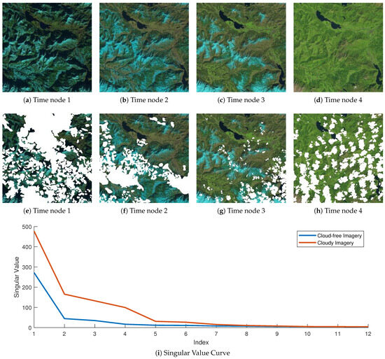
Figure 1.
(a–d) The images in cloud-free Munich dataset of 4 time nodes. (e–h) The simulated cloudy Munich dataset with different cloud masks. (i) The singular value curves for the cloud-free and cloudy imagery. Note that for time nodes 1 to 4, the exact timestamps are 201501, 201503, 201504 and 201508, where “XXXXYY” means the image is taken in YY-th month of XXXX-th year.
Therefore, the thick cloud removal task can be typically formulated as a low-rank matrix/tensor completion problem, where the pixels covered by clouds are regarded as missing pixels. The existing algorithms (e.g., TNN) exhibit remarkable performance on low-rank tensor completion problems. However, they are computationally intensive. To develop a faster algorithm, this paper focuses on the matrix format. The most classical approach to exploring low-rank properties of matrix data is the low-rank matrix factorization technique. Given a predefined integer r, the recovered cloud-free data can be expressed as [40], where represents the representation coefficients and denotes the basis of the subspace. Note that it is often assumed that so that the rank of is r, leading to low-rank matrix factorization. This mathematical expression may be unreadable for readers who do not excel at low-rank data analysis. Actually, the formula can be regarded as spectral unmixing [41], where U denotes the abundance matrix, V denotes the endmember matrix and r represents the number of endmembers.
Since the cloud-free image is inaccessible, X is an unknown variable that needs estimation. To this end, the cloud removal task can be formulated as:
where is an index set collecting all the pixels that are not covered by clouds. Note that is an orthogonal projection operator. In other words, if a pixel is not covered by cloud (), the projection will return its value; otherwise, the projection will return zero.
In Equation (1), the loss function encourages the recovered image X to be low rank, and the constraint forces the recovered and observed imagesto exhibit the same pixel values for regions not covered by clouds. This optimization is typically solved via the ADMM algorithm, where the key step involves implementing singular value decomposition (SVD) with the computational complexity of .
The model in Equation (1) is typically fast but insufficient for recovering complex textures. To enhance texture quality, a common strategy is to incorporate the local smoothness prior (i.e., neighbor pixels tend to have similar values). In other words, the total variation is imposed on X, resulting in the following problem:
Here, is a hyperparameter, and the total variation is defined as:
where represents the tensor version of X, and and denote the horizontal and vertical gradient operators, respectively. In other words, and represent the difference between two neighbor pixels along horizontal and vertical directions. Minimizing the TV regularizer facilitates neighbor pixels to have similar values, potentially leading to better image quality. It is well known that the total variation minimization problem is often solved by using the fast Fourier transform (FFT) with a computational complexity of [42]. However, despite the significant improvement in total variation, the high computational complexity is undesirable. This urges researchers to explore fast and high-performance algorithms.
2.2. Representation Coefficient Total Variation
To reduce computational complexity, this paper presents an investigation into a novel regularizer. We first demonstrate that the representation coefficient U (abundance matrix) is visually akin to images. This assertion is substantiated by the first row of Figure 2, where the Munich dataset is decomposed with , yielding five coefficients. It is evident that each coefficient conveys a similar context in the original images depicted in Figure 2. Next, we pose an intriguing question: do these coefficients exhibit local smoothness? To address this, we visualize the gradient intensity map in the second row of Figure 2. The gradient intensity of pixel is defined as:
and its histogram is presented in the third row of Figure 2. The analysis reveals that the gradient intensities of most pixels approach zero, indicating that the coefficients U are locally smooth.
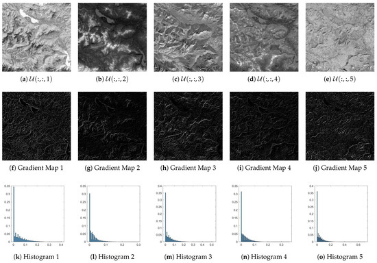
Figure 2.
(a–e) The visualization for 5 representation coefficients. (f–j) The gradient map of each representation coefficient. For easier inspection, the value of the gradient map is amplified 2 times. (k–o) The histogram of each representation coefficient.
Building upon this discovery, this paper introduces a novel regularizer, representation coefficient total variation (RCTV), characterized by the following definition:
where represents the tensor counterpart of U. In contrast to Equation (3), RCTV applies the -norm to the gradients of the coefficients U rather than X. Although the difference between TV and RCTV seems to appear minimal, it should be emphasized that this variant is not trivial:
Firstly, the RCTV minimization problem is addressed by FFT, accompanied by a relatively lower computational complexity of . This is attributed to the assumption that . This advantage becomes particularly significant when the number of channels or time nodes is substantial. More significantly, when generating cloud-free data under the constraint , the algorithm essentially only estimates the pixels obscured by clouds, directly copying their values if they are cloud-free. As TV is applied to the entire dataset [31,43], it consumes computational resources excessively for cloud-free pixels. However, RCTV mitigates this issue to a certain extent since it is imposed on representation coefficients.
Secondly, the resulting data are ultimately reconstructed through the product of U and , which potentially maintains gradient map consistency across different channels and time nodes. That is to say, different channels and time nodes will exhibit similar texture and structure, so RCTV can more efficiently exploit information from other channels and time nodes. However, TV solely employs local smoothness within a single channel at each time node. In this regard, RCTV appears more promising in extracting additional texture information from different channels and time nodes.
2.3. RCTV-Regularized Cloud Removal
Subsequently, the RCTV-regularized cloud removal (RCTVCR) model is formulated as:
Compared with Equation (2), the above equation minimizes RCTV instead of TV, and it inserts a constraint for stability.
To solve this problem, two auxiliary variables and are introduced to decouple the -norm and , resulting in the following problem:
The ADMM algorithm is employed to solve this problem, aiming to minimize the augmented Lagrangian function of the above problem. That is,
Note that and M are Lagrangian multipliers, and is the penalty parameter. We then update each variable alternatively.
Update : by fixing other variables, we focus on optimizing . The corresponding optimization problem is as follows:
The solution is given by:
where the soft-thresholding function .
Update U: this leads to the following optimization problem:
Setting the derivative of this objective function to zero yields the optimal solution equation:
where denotes the transposed operator of . After simplification, the equation becomes:
where represents the unfolding operation. For clarity, the right-hand side of this equation is denoted by R. By applying the FFT on both sides and the convolution theorem, the closed-form solution can be derived as [44]:
Here, represents the FFT, and denotes the element-wise square operation.
Update V: the optimization problem concerning V is formulated as:
After straightforward calculation, the problem can be rewritten as:
Drawing upon reference [45], the solution can be derived as:
Update X: the problem is a constrained least-squares task:
The solution can be straightforwardly obtained as:
Update multipliers: based on the general ADMM principle, the multipliers are further updated using the following equations:
Finally, Algorithm 1 summarizes the workflow.
| Algorithm 1 RCTVCR. |
| Require: Ensure:X Initialize U and V via truncated SVD. Set multipliers , and M to zero tensors/matrices. Set and . for do Update . Update . Update . Carry out SVD on , i.e., . Update . Update . Update multipliers by Update . if then BREAK end if end for |
3. Experiments
To assess the performance of the RCTVCR algorithm, experiments are conducted on both synthetic and real-world datasets. Peak signal-to-noise ratio (PSNR), structure similarity (SSIM) and spectral angle mapper (SAM) are employed for evaluation purposes. Higher PSNR and SSIM and lower SAM mean that the image has better quality. The compared methods include HaLRTC [16,17], SNNTV [46], SPCTV [47], TNN [18,19] and FTNN [23]. All experiments are conducted on a desktop running Windows 10, equipped with an Intel Core i7-12700F CPU at 2.10 GHz and 32 GB of memory.
3.1. Experiment on Synthetic Datasets
In this subsection, a comprehensive series of synthetic experiments are performed to assess the effectiveness of RCTVCR. The synthetic datasets consist of Munich with three channels and four time nodes, and Farmland with eight channels and four time nodes. Figure 3 illustrates the images from the Farmland dataset. These datasets comprise pixels and were captured via Landsat-8. To enhance realism, three real cloud masks with varying cloud amounts are chosen from the WHU cloud dataset, as presented in Figure 4.
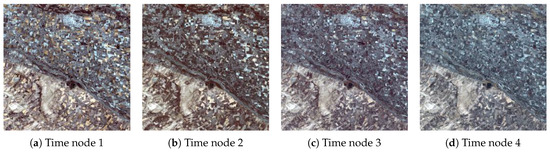
Figure 3.
The false-color images in Farmland dataset. Note that for time nodes 1 to 4, the exact timestamps are 20130715, 20130901, 20131003 and 20131019, where “XXXXYYZZ” means the image is taken in ZZ-th day of YY-th month of XXXX-th year.
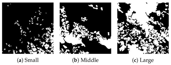
Figure 4.
The three cloud masks with different-sized clouds. The white pixels denote clouds.
Table 1 summarizes the performance comparison of all competing methods in terms of performance metrics (PSNR, SSIM and processing time) on the Munich dataset. As the cloud mask size increases from small to large, the PSNR and SSIM values for all methods generally decrease. Based on the results presented in the table, it can be inferred that RCTVCR emerges as the optimal method due to its consistent achievement of the highest PSNR and SSIM values across all cloud mask sizes, accompanied by the shortest processing time.

Table 1.
Metrics on Munich dataset. The best values are marked in bold.
Table 2 displays a comparative analysis of various methods in terms of their performance metrics on the Farmland dataset. Similar to the Munich dataset, a consistent pattern is observed: as the cloud mask size escalates from small to large, the PSNR and SSIM values for all methods generally decrease. When comparing RCTVCR with SPCTV and TNN, it is noticeable that RCTVCR exhibits a higher PSNR value by 0.35 and 0.44, respectively, on the large cloud mask size. Moreover, RCTVCR boasts the shortest processing time. Only 0.2 s is required to process the Farmland dataset with a large mask, whereas SPCTV and TNN necessitate 394.3 s and 176.3 s, respectively. Based on these results, it can be concluded that RCTVCR emerges as the optimal method, consistently achieving the highest PSNR and SSIM values.
Table 2.
Metrics on Farmland dataset. The best values are marked in bold.
To further emphasize the superiority of our method, we present the declouded images of Munich and Farmland in Figure 5 and Figure 6. Our method effectively preserves intricate details and yields more visually appealing outcomes, whereas competing methods often result in blurred or artificial-looking artifacts. It should be noted that compared methods that are based on tensor factorization or tensor nuclear norms exhibit varying degrees of checkerboard artifacts. RCTVCR, however, exhibits no such disadvantage.
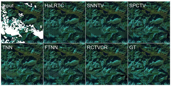
Figure 5.
The false-color decloud images of all compared methods using Munich dataset with a middle cloud mask.
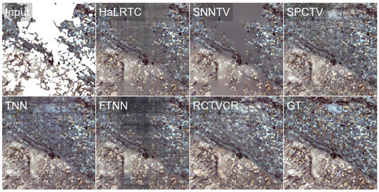
Figure 6.
The false-color decloud images of all compared methods on Farmland dataset with a large cloud mask.
To better illustrate the efficiency of RCTVCR, a scatter plot is visualized in Figure 7 for the Farmland dataset with a middle cloud mask. It is shown that RCTVCR achieves the highest PSNR with the fastest speed. TNN and SPCTV obtain improvements over HaLRTC at the cost of a very long processing time. FTNN is the most computationally intensive, but it has an unsatisfactory PSNR value. The reason may be that FTNN is more suitable for random missing completion tasks. Nonetheless, the clouds correspond to continuous area missing completion tasks, which is more challenging.
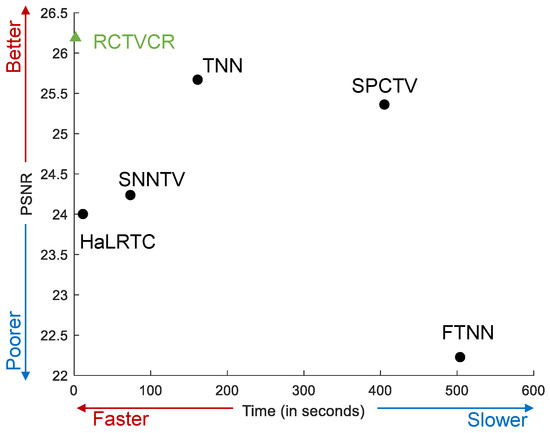
Figure 7.
The scatter plot of PSNR and time for the Farmland dataset with a middle cloud mask.
In conclusion, the superior visual performance of our method relative to existing techniques is clearly demonstrated through experimental outcomes. By effectively tackling cloud removal, structural preservation and overall image quality enhancement, our proposed approach represents an advancement in the field.
3.2. Experiments on Real-World Datasets
Here, we apply competing methods to a real-world dataset, which was released in [39]. It was captured via Sentinel-2 over Mechelen, Belgium. The original data size is very large, and thus, a patch with a size of is cropped. There are three channels and seven time nodes, and cloudy images and corresponding masks are displayed in Figure 8. It is revealed that time nodes 2, 5 and 7 are polluted by severe clouds and shadows, which would be a very difficult task. Former investigations often select partial time nodes with fewer clouds to verify algorithm performance. In our study, all time nodes are simultaneously employed to test algorithm robustness to the amount of cloud coverage.
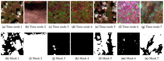
Figure 8.
The false-color images and their masks in the real-world dataset. Note that for time nodes 1 to 7, the exact timestamps are 20180816, 20180831, 20180905, 20180915, 20180925, 20181015 and 20181020, where “XXXXYYZZ” means the image is taken on ZZ-th day of YY-th month of XXXX-th year.
Decloud images are displayed in Figure 9. It is observed that HaLRTC and SNNTV output very blurry contexts. FTNN could recover a few more details, but it cannot accurately remove clouds and shadows. SPCTV and TNN exhibit heavy checkerboard effects and color distortion. Only our method faithfully recovers plenty of details and preserves color consistency. Additionally, the barplot shown in Figure 10 reveals that RCTVCR with a processing time of 6 s is significantly faster than other methods, which often take hundreds of seconds.
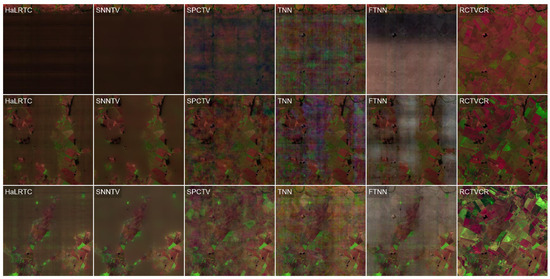
Figure 9.
The false-color decloud images of all compared methods on the real-world dataset. From top to bottom, they correspond to time nodes 2, 5 and 7, respectively.
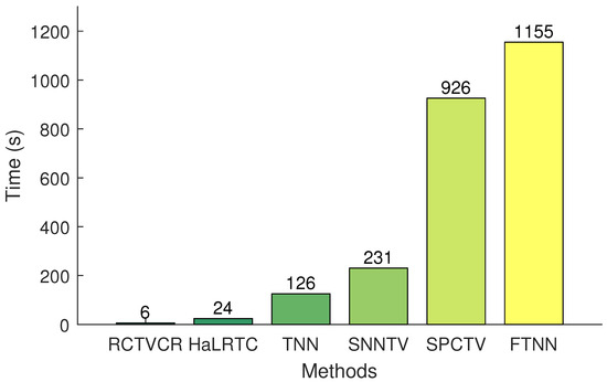
Figure 10.
The processing time on real-world data with a size of .
4. Discussions
4.1. Influence of the Temporal Number
To assess the impact of the temporal number on the reconstruction effectiveness of our method, we conducted the following experiment. We maintain the cloudy image of the Munich dataset with a middle mask and gradually add reference images to vary the temporal number. Table 3 presents three metrics of the decloud images using reference images with varying temporal numbers. The data indicate that as the temporal number grows, the image quality also increases. However, from Table 1, it is shown that RCTVCR with a smaller temporal number is still better than some existing methods with four time nodes, validating the effectiveness of RCTVCR.
Table 3.
Metrics on Munich dataset of RCTVCR with varying temporal number.
4.2. Parameter Sensitivity
In RCTVCR, two parameters, r and , require tuning. To examine the impact of these parameters, we implemented RCTVCR with various parameter configurations on the Farmland dataset with a middle cloud mask.
Initially, we fixed at and varied r from 12 to 22. As depicted in Figure 11a, the PSNR curve rapidly increased before gradually descending as r increased, achieving optimal performance at . Figure 12 displays the declouded images obtained with , 14 and 22. It is evident that yields superior details compared to . Notably, preserves decent textures but exhibits color distortion.
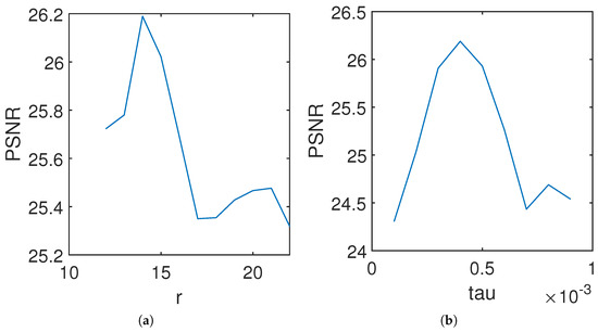
Figure 11.
The metric with different hyper-parameters.
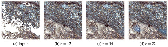
Figure 12.
The decloud images with and different r.
Subsequently, we fixed and investigated values ranging from to . As illustrated in Figure 11b, the PSNR curve incrementally increased before exhibiting a tendency to decline as increased, yielding the optimal performance at . The declouded images with , and are presented in Figure 13. It should be noted that governs the strength of the RCTV regularizer. A small value of leads to similarity in the behavior of RCTVCR and methods that do not employ a local smoothness prior (e.g., HaLRTC). Conversely, a large value of results in a relatively blurry image.
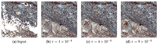
Figure 13.
The decloud images with and different values.
5. Conclusions
In conclusion, the proposed method for removing thick clouds from remote sensing images offers an effective and efficient solution. By employing matrix decomposition and regularization techniques, the method not only removes thick clouds but also preserves the textures in the images, resulting in improved visual quality. The sensitivity analysis and comparisons with other methods further validate the superiority of the proposed approach. This study contributes to the advancement of remote sensing image processing and has potential applications in various fields. Further research can be conducted to enhance the method’s robustness and applicability in different scenarios. Due to the current limitations of our research scope and hardware resources, we are unable to incorporate deep learning techniques into our experimental comparison at this stage. Future work includes exploring possible avenues for incorporating deep learning methods into our research.
Author Contributions
Conceptualization, S.X.; methodology, S.X.; software, J.W. (Jilong Wang); validation, J.W. (Jialin Wang); formal analysis, J.W. (Jialin Wang); writing—original draft preparation, J.W. (Jialin Wang); writing—review and editing, S.X.; visualization, J.W. (Jilong Wang). All authors have read and agreed to the published version of the manuscript.
Funding
This research was funded by Research Fund of Guangxi Key Lab of Multi-source Information Mining & Security (grant number: MIMS22-16), Fundamental Research Funds for the Central Universities (grant number: D5000220060), the National Natural Science Foundation of China (grant number: 12201497), the Guangdong Basic and Applied Basic Research Foundation (grant number: 2023A1515011358) and the Shaanxi Fundamental Science Research Project for Mathematics and Physics (grant number: 22JSQ033).
Data Availability Statement
Data available on request from the authors.
Conflicts of Interest
The authors declare no conflicts of interest.
References
- Zhang, Q.; Yuan, Q.; Li, J.; Li, Z.; Shen, H.; Zhang, L. Thick cloud and cloud shadow removal in multitemporal imagery using progressively spatio-temporal patch group deep learning. ISPRS J. Photogramm. Remote Sens. 2020, 162, 148–160. [Google Scholar] [CrossRef]
- Cao, R.; Chen, Y.; Chen, J.; Zhu, X.; Shen, M. Thick cloud removal in Landsat images based on autoregression of Landsat time-series data. Remote Sens. Environ. 2020, 249, 112001. [Google Scholar] [CrossRef]
- Xu, S.; Cao, X.; Peng, J.; Ke, Q.; Ma, C.; Meng, D. Hyperspectral Image Denoising by Asymmetric Noise Modeling. IEEE Trans. Geosci. Remote Sens. 2022, 60, 1–14. [Google Scholar] [CrossRef]
- Li, J.; Hu, Q.; Ai, M. Haze and thin cloud removal via sphere model improved dark channel prior. IEEE Geosci. Remote Sens. Lett. 2018, 16, 472–476. [Google Scholar] [CrossRef]
- Zhu, X.; Gao, F.; Liu, D.; Chen, J. A modified neighborhood similar pixel interpolator approach for removing thick clouds in Landsat images. IEEE Geosci. Remote Sens. Lett. 2011, 9, 521–525. [Google Scholar] [CrossRef]
- Li, J.; Zhang, Y.; Sheng, Q.; Wu, Z.; Wang, B.; Hu, Z.; Shen, G.; Schmitt, M.; Molinier, M. Thin Cloud Removal Fusing Full Spectral and Spatial Features for Sentinel-2 Imagery. IEEE J. Sel. Top. Appl. Earth Obs. Remote Sens. 2022, 15, 8759–8775. [Google Scholar] [CrossRef]
- Li, W.; Li, Y.; Chan, J.C.W. Thick cloud removal with optical and SAR imagery via convolutional-mapping-deconvolutional network. IEEE Trans. Geosci. Remote Sens. 2019, 58, 2865–2879. [Google Scholar] [CrossRef]
- Tao, C.; Fu, S.; Qi, J.; Li, H. Thick cloud removal in optical remote sensing images using a texture complexity guided self-paced learning method. IEEE Trans. Geosci. Remote Sens. 2022, 60, 1–12. [Google Scholar] [CrossRef]
- Xu, M.; Jia, X.; Pickering, M.; Plaza, A.J. Cloud removal based on sparse representation via multitemporal dictionary learning. IEEE Trans. Geosci. Remote Sens. 2016, 54, 2998–3006. [Google Scholar] [CrossRef]
- Zhu, X.; Kang, Y.; Liu, J. Estimation of the number of endmembers via thresholding ridge ratio criterion. IEEE Trans. Geosci. Remote Sens. 2019, 58, 637–649. [Google Scholar] [CrossRef]
- Lin, C.H.; Tsai, P.H.; Lai, K.H.; Chen, J.Y. Cloud removal from multitemporal satellite images using information cloning. IEEE Trans. Geosci. Remote Sens. 2012, 51, 232–241. [Google Scholar] [CrossRef]
- Lin, C.H.; Lai, K.H.; Chen, Z.B.; Chen, J.Y. Patch-based information reconstruction of cloud-contaminated multitemporal images. IEEE Trans. Geosci. Remote Sens. 2013, 52, 163–174. [Google Scholar] [CrossRef]
- Cheng, Q.; Shen, H.; Zhang, L.; Yuan, Q.; Zeng, C. Cloud removal for remotely sensed images by similar pixel replacement guided with a spatio-temporal MRF model. ISPRS J. Photogramm. Remote Sens. 2014, 92, 54–68. [Google Scholar] [CrossRef]
- Chen, B.; Huang, B.; Chen, L.; Xu, B. Spatially and temporally weighted regression: A novel method to produce continuous cloud-free Landsat imagery. IEEE Trans. Geosci. Remote Sens. 2016, 55, 27–37. [Google Scholar] [CrossRef]
- Shi, J. Active Microwave Remote Sensing Systems and Applications to Snow Monitoring. In Advances in Land Remote Sensing: System, Modeling, Inversion and Application; Liang, S., Ed.; Springer: Dordrecht, The Netherlands, 2008; pp. 19–49. [Google Scholar]
- Liu, J.; Musialski, P.; Wonka, P.; Ye, J. Tensor completion for estimating missing values in visual data. In Proceedings of the IEEE 12th International Conference on Computer Vision, ICCV 2009, Kyoto, Japan, 27 September–4 October 2009; pp. 2114–2121. [Google Scholar]
- Liu, J.; Musialski, P.; Wonka, P.; Ye, J. Tensor Completion for Estimating Missing Values in Visual Data. IEEE Trans. Pattern Anal. Mach. Intell. 2013, 35, 208–220. [Google Scholar] [CrossRef] [PubMed]
- Lu, C.; Feng, J.; Chen, Y.; Liu, W.; Lin, Z.; Yan, S. Tensor Robust Principal Component Analysis: Exact Recovery of Corrupted Low-Rank Tensors via Convex Optimization. In Proceedings of the 2016 IEEE Conference on Computer Vision and Pattern Recognition, CVPR 2016, Las Vegas, NV, USA, 27–30 June 2016; pp. 5249–5257. [Google Scholar]
- Lu, C.; Feng, J.; Lin, Z.; Yan, S. Exact Low Tubal Rank Tensor Recovery from Gaussian Measurements. In Proceedings of the Twenty-Seventh International Joint Conference on Artificial Intelligence, IJCAI 2018, Stockholm, Sweden, 13–19 July 2018; Lang, J., Ed.; pp. 2504–2510. [Google Scholar]
- Lu, C.; Feng, J.; Chen, Y.; Liu, W.; Lin, Z.; Yan, S. Tensor Robust Principal Component Analysis with a New Tensor Nuclear Norm. IEEE Trans. Pattern Anal. Mach. Intell. 2020, 42, 925–938. [Google Scholar] [CrossRef]
- Cai, J.F.; Chan, R.H.; Shen, Z. A framelet-based image inpainting algorithm. Appl. Comput. Harmon. Anal. 2008, 24, 131–149. [Google Scholar] [CrossRef]
- Jiang, T.X.; Huang, T.Z.; Zhao, X.L.; Ji, T.Y.; Deng, L.J. Matrix factorization for low-rank tensor completion using framelet prior. Inf. Sci. 2018, 436, 403–417. [Google Scholar] [CrossRef]
- Jiang, T.; Ng, M.K.; Zhao, X.; Huang, T. Framelet Representation of Tensor Nuclear Norm for Third-Order Tensor Completion. IEEE Trans. Image Process. 2020, 29, 7233–7244. [Google Scholar] [CrossRef]
- Ji, T.; Yokoya, N.; Zhu, X.X.; Huang, T. Nonlocal Tensor Completion for Multitemporal Remotely Sensed Images’ Inpainting. IEEE Trans. Geosci. Remote Sens. 2018, 56, 3047–3061. [Google Scholar] [CrossRef]
- Chen, Y.; He, W.; Yokoya, N.; Huang, T.Z. Blind cloud and cloud shadow removal of multitemporal images based on total variation regularized low-rank sparsity decomposition. ISPRS J. Photogramm. Remote Sens. 2019, 157, 93–107. [Google Scholar] [CrossRef]
- Duan, C.; Pan, J.; Li, R. Thick cloud removal of remote sensing images using temporal smoothness and sparsity regularized tensor optimization. Remote Sens. 2020, 12, 3446. [Google Scholar] [CrossRef]
- Dao, M.; Kwan, C.; Ayhan, B.; Tran, T.D. Burn scar detection using cloudy MODIS images via low-rank and sparsity-based models. In Proceedings of the 2016 IEEE Global Conference on Signal and Information Processing (GlobalSIP), Washington, DC, USA, 7–9 December 2016; pp. 177–181. [Google Scholar] [CrossRef]
- Zhao, Q.; Zhang, L.; Cichocki, A. Bayesian CP factorization of incomplete tensors with automatic rank determination. IEEE Trans. Pattern Anal. Mach. Intell. 2015, 37, 1751–1763. [Google Scholar] [CrossRef] [PubMed]
- Luo, Q.; Han, Z.; Chen, X.; Wang, Y.; Meng, D.; Liang, D.; Tang, Y. Tensor rpca by bayesian cp factorization with complex noise. In Proceedings of the IEEE International Conference on Computer Vision, Venice, Italy, 22–29 October 2017; pp. 5019–5028. [Google Scholar]
- Mørup, M. Applications of tensor (multiway array) factorizations and decompositions in data mining. Wiley Interdiscip. Rev. Data Min. Knowl. Discov. 2011, 1, 24–40. [Google Scholar] [CrossRef]
- He, W.; Yokoya, N.; Yuan, L.; Zhao, Q. Remote Sensing Image Reconstruction Using Tensor Ring Completion and Total Variation. IEEE Trans. Geosci. Remote Sens. 2019, 57, 8998–9009. [Google Scholar] [CrossRef]
- Lin, J.; Huang, T.Z.; Zhao, X.L.; Chen, Y.; Zhang, Q.; Yuan, Q. Robust thick cloud removal for multitemporal remote sensing images using coupled tensor factorization. IEEE Trans. Geosci. Remote Sens. 2022, 60, 1–16. [Google Scholar] [CrossRef]
- Zheng, Y.B.; Huang, T.Z.; Zhao, X.L.; Zhao, Q.; Jiang, T.X. Fully-connected tensor network decomposition and its application to higher-order tensor completion. In Proceedings of the AAAI Conference on Artificial Intelligence, Virtual, 2–9 February 2021; Volume 35, pp. 11071–11078. [Google Scholar]
- Zheng, W.J.; Zhao, X.L.; Zheng, Y.B.; Lin, J.; Zhuang, L.; Huang, T.Z. Spatial-spectral-temporal connective tensor network decomposition for thick cloud removal. ISPRS J. Photogramm. Remote Sens. 2023, 199, 182–194. [Google Scholar] [CrossRef]
- Mazza, A.; Ciotola, M.; Poggi, G.; Scarpa, G. Synergic Use of SAR and Optical Data for Feature Extraction. In Proceedings of the IEEE International Geoscience and Remote Sensing Symposium, IGARSS 2023, Pasadena, CA, USA, 16–21 July 2023; pp. 2061–2064. [Google Scholar]
- Scarpa, G.; Gargiulo, M.; Mazza, A.; Gaetano, R. A CNN-Based Fusion Method for Feature Extraction from Sentinel Data. Remote Sens. 2018, 10, 236. [Google Scholar] [CrossRef]
- Singh, P.; Komodakis, N. Cloud-Gan: Cloud Removal for Sentinel-2 Imagery Using a Cyclic Consistent Generative Adversarial Networks. In Proceedings of the IGARSS 2018—2018 IEEE International Geoscience and Remote Sensing Symposium, Valencia, Spain, 22–27 July 2018; pp. 1772–1775. [Google Scholar] [CrossRef]
- Ebel, P.; Meraner, A.; Schmitt, M.; Zhu, X.X. Multisensor Data Fusion for Cloud Removal in Global and All-Season Sentinel-2 Imagery. IEEE Trans. Geosci. Remote Sens. 2021, 59, 5866–5878. [Google Scholar] [CrossRef]
- Zhang, Q.; Yuan, Q.; Li, Z.; Sun, F.; Zhang, L. Combined deep prior with low-rank tensor SVD for thick cloud removal in multitemporal images. ISPRS J. Photogramm. Remote Sens. 2021, 177, 161–173. [Google Scholar] [CrossRef]
- Liu, J.; Yuan, S.; Zhu, X.; Huang, Y.; Zhao, Q. Nonnegative matrix factorization with entropy regularization for hyperspectral unmixing. Int. J. Remote Sens. 2021, 42, 6359–6390. [Google Scholar] [CrossRef]
- Bioucas-Dias, J.M.; Plaza, A.; Dobigeon, N.; Parente, M.; Du, Q.; Gader, P.D.; Chanussot, J. Hyperspectral Unmixing Overview: Geometrical, Statistical, and Sparse Regression-Based Approaches. IEEE J. Sel. Top. Appl. Earth Obs. Remote Sens. 2012, 5, 354–379. [Google Scholar] [CrossRef]
- Peng, J.; Wang, H.; Cao, X.; Liu, X.; Rui, X.; Meng, D. Fast noise removal in hyperspectral images via representative coefficient total variation. IEEE Trans. Geosci. Remote Sens. 2022, 60, 1–17. [Google Scholar] [CrossRef]
- Xu, S.; Zhang, J.; Zhang, C. Hyperspectral image denoising by low-rank models with hyper-Laplacian total variation prior. Signal Process. 2022, 201, 108733. [Google Scholar] [CrossRef]
- Krishnan, D.; Fergus, R. Fast image deconvolution using hyper-Laplacian priors. Adv. Neural Inf. Process. Syst. 2009, 22, 1033–1041. [Google Scholar]
- Peng, J.; Xie, Q.; Zhao, Q.; Wang, Y.; Yee, L.; Meng, D. Enhanced 3DTV regularization and its applications on HSI denoising and compressed sensing. IEEE Trans. Image Process. 2020, 29, 7889–7903. [Google Scholar] [CrossRef]
- Li, X.; Ye, Y.; Xu, X. Low-Rank Tensor Completion with Total Variation for Visual Data Inpainting. In Proceedings of the Thirty-First AAAI Conference on Artificial Intelligence, San Francisco, CA, USA, 4–9 February 2017; Singh, S., Markovitch, S., Eds.; AAAI Press: Washington, DC, USA, 2017; pp. 2210–2216. [Google Scholar]
- Yokota, T.; Zhao, Q.; Cichocki, A. Smooth PARAFAC Decomposition for Tensor Completion. IEEE Trans. Signal Process. 2016, 64, 5423–5436. [Google Scholar] [CrossRef]
Disclaimer/Publisher’s Note: The statements, opinions and data contained in all publications are solely those of the individual author(s) and contributor(s) and not of MDPI and/or the editor(s). MDPI and/or the editor(s) disclaim responsibility for any injury to people or property resulting from any ideas, methods, instructions or products referred to in the content. |
© 2023 by the authors. Licensee MDPI, Basel, Switzerland. This article is an open access article distributed under the terms and conditions of the Creative Commons Attribution (CC BY) license (https://creativecommons.org/licenses/by/4.0/).