

FEPVNet: A Network with Adaptive Strategies for Cross-Scale Mapping of Photovoltaic Panels from Multi-Source Images
by
 , , , ,
Buyu Su
1,2,3,
Xiaoping Du
1,2,*,
Haowei Mu
4,
Chen Xu
1,2,
Xuecao Li
5,
Fang Chen
1,2 and
Xiaonan Luo
3 1
Key Lab of Digital Earth Sciences, Aerospace Information Research Institute, Chinese Academy of Sciences, Beijing 100094, China
2
International Research Center of Big Data for Sustainable Development Goals, Beijing 100094, China
3
School of Computer Science and Information Security, Guilin University of Electronic Technology, Guilin 541004, China
4
School of Geography and Ocean Science, Nanjing University, Nanjing 210023, China
5
College of Land Science and Technology, China Agricultural University, Beijing 100094, China
*
Author to whom correspondence should be addressed.
Remote Sens. 2023, 15(9), 2469; https://doi.org/10.3390/rs15092469
Submission received: 27 March 2023
/
Revised: 27 April 2023
/
Accepted: 5 May 2023
/
Published: 8 May 2023
(This article belongs to the Special Issue Remote Sensing Image Scene Classification Meets Artificial Intelligence)
Abstract
:The world is transitioning to renewable energy, with photovoltaic (PV) solar power being one of the most promising energy sources. Large-scale PV mapping provides the most up-to-date and accurate PV geospatial information, which is crucial for planning and constructing PV power plants, optimizing energy structure, and assessing the ecological impact of PVs. However, previous methods of PV extraction relied on simple models and single data sources, which could not accurately obtain PV geospatial information. Therefore, we propose the Filter-Embedded Network (FEPVNet), which embeds high-pass and low-pass filters and Polarized Self-Attention (PSA) into a High-Resolution Network (HRNet) to improve its noise resistance and adaptive feature extraction capabilities, ultimately enhancing the accuracy of PV extraction. We also introduce three data migration strategies by combining Sentinel-2, Google-14, and Google-16 images in varying proportions and transferring the FEPVNet trained on Sentinel-2 images to Gaofen-2 images, which improves the generalization performance of models trained on a single data source for extracting PVs in images of different scales. Our model improvement experiments demonstrate that the Intersection over Union (IoU) of FEPVNet in segmenting China PVs in Sentinel-2 images reaches 88.68%, a 2.37% increase compared to the HRNet. Furthermore, we use FEPVNet and the optimal migration strategy to extract photovoltaics across scales, achieving a precision of 94.37%. In summary, this study proposes the FEPVNet model with adaptive strategies for extracting PVs from multiple image sources, with significant potential for application in large-scale PV mapping.
1. Introduction
The global demand for energy is facing significant challenges and uncertainties, manifested by the decrease in fossil energy reserves and rising prices [1]. Moreover, the burning of fossil energy sources emits large amounts of carbon dioxide, which leads to atmospheric pollution [2]. As a result, countries are turning to renewable energy sources, particularly solar energy due to its universality, harmlessness, and immensity and permanence [3].
According to the International Energy Agency’s (IEA) sustainability program, the number of photovoltaic (PV) plants will increase rapidly, taking up much land [4]. However, potential problems can be induced during the process of PV industry development, such as competition for land with PV deployment due to increased human activity and damage to biodiversity and the climate due to land change in PV regions [5]. Consequently, the accurate geo-spatial location of PVs is critical for assessing past impacts and planning to avoid future conflicts.
With the development of satellite sensor technology, many remote-sensing images have been acquired for PV extraction. PV panels can be detected and segmented from remote-sensing images by designing representative features (e.g., color, geometry, and texture) using the threshold segmentation algorithm [6,7], the edge detection algorithm [8,9], or the SVM algorithm in machine learning [10,11]. However, these features vary due to the atmospheric conditions, lighting, and observation scales, resulting in weak accuracy and the generalization of traditional methods [12,13]. Moreover, PV plants have been built in various landscapes (e.g., deserts, mountains, and coasts) [14,15,16]. This makes it challenging to accurately identify PVs on a continental scale. Therefore, more than the traditional method is required to cope with these situations [17].
Deep learning (DL) has been favored in view of its success in object detection and segmentation for remote-sensing areas [18,19]. Many researchers began using convolutional neural networks (CNNs) for scene classification, crop yield prediction, and land cover, among other jobs [20,21,22]. For PV extraction, several CNNs were used to localize PVs from remote-sensing images and estimate their sizes [23,24,25,26]. For example, Yuan et al. [27] completed large-scale PV segmentation based on CNNs. Jumaboev et al. [28] compared the PV segmentation effect of deeplabv3+, FPN, and U-Net. However, the above studies focused on using the original DL models without analyzing the characteristics of PV image or improving the models. Therefore, there is a gap in further improving DL methods’ segmentation accuracy and robustness (i.e., the adaptive model design and data combination).
In recent years, the development of computer hardware and remote-sensing technology [29,30,31] has provided a solid foundation for large-scale PV mapping (e.g., global, regional) [17,32]. Based on this, we need to design the CNN model to acquire PV features from multi-source remote-sensing images adaptively, in order to complete PV extraction from different regions and scales [6,33,34]. In addition, attention is used to observe crucial local information and combine it with information from other regions to form an overall understanding of the object, thereby enhancing the feature extraction ability. Currently, attention is extensively employed in DL models for remote-sensing image processing to make the model adaptive in acquiring the critical features of the object [35,36,37].
Previous methods have been primarily focused on PV extraction from a single data source and have achieved impressive performance. However, these methods are insufficient to cope with the multi-sourcing of remote-sensing images. The above literature has not widely analyzed the cross-scale extraction of PVs from multi-source images. This study examined the current mainstream CNN models. Many researchers have compared U-Net, DeepLabv3+, PSPNet, and HRNet models on the PASCAL VOC 2012 dataset, and HRNet achieved the best performance [38,39]. Therefore, we selected HRNet as the base model and embedded Canny, Median filter, and Polarized Self-Attention (PSA) to design an adaptive FEPVNet. We tested the effectiveness of FEPVNet in PV extraction from Sentinel-2 images and conducted cross-validation using different PV region models. Finally, we constructed three data migration strategies by combining multi-source data and employed the model trained on Sentinel-2 images for PV extraction from Gaofen-2 images, and its Precision reached 94.37%. Our cross-scale PV extraction method is expected to contribute to the large-scale mapping of PV in the future.
2. Datasets
To construct the cross-scale network model, four types of images are required: a Sentinel-2 image at a 10 m resolution, which is available for download via Google Earth Engine (GEE), a Google-14 (i.e., zoom level is 14) image at a 10 m resolution, a Google-16 (i.e., zoom level is 16) image at a 2 m resolution, all of which can be downloaded through the Google Images’ API, and a Gaofen-2 image at a 2 m resolution, which can be downloaded from the Data Sharing Website of Aerospace Information Research Institute, Chinese Academy of Sciences. Therefore, we first validated the FEPVNet performance using the Sentinel-2 images, then constructed three data migration strategies using the Sentinel-2 and Google images, and finally completed the PV extraction from the Goafen-2 images.
We utilized the PV location information from the open-source global PV installation list [32] to select the vector sample with PVs. The above four categories of raster images were downloaded according to the boundaries of these vector samples, and the vector samples were transformed into PV labels of the corresponding category. The labels with incorrect PV boundaries were redrawn using LabelMe. The sample images of Sentinel-2 that we used consist of three bands: red (B4), green (B3), and blue (B2), while the sample label images are grayscale images. These images were cut into 1024 × 1024 pixels, forming four datasets with properties shown in Table 1. The dataset was divided into three parts, one training set, one validation set, and one test set. The results were poor when training the model on Sentinel-2 images and directly extracting PVs from Gaofen-2 images. Therefore, we consider combining multiple PV features to complete the transfer work of the Sentinel-2 model. We aimed to utilize the images from Sentinel-2 and Google of different resolutions to perform cross-scale PV extraction in Gaofen-2 imagery without using Gaofen-2 imagery to train the model. As a result, only the training set of Google images was needed. For model training, we used Gaofen-2 imagery as the validation set and test set. Thus, Google images did not require validation and test sets, and Gaofen-2 imagery did not need a training set. Finally, we used data augmentation such as rotation, color transformation, and noise injection to augment the dataset.
3. Methodology
The methodology framework consists of five parts as shown in Figure 1: (a) completing the PV dataset by converting the vector samples into labels for the multi-source images, (b) validating the advantages of our improved module through ablation experiments of FEPVNet, (c) comparing the PV extraction ability of different models on the Sentinel-2 dataset, (d) using FEPVNet for cross-validation of the Sentinel-2 images in different regions, and (e) completing a PV cross-scale extraction from multi-source remote-sensing images using FEPVNet and the migration strategy.
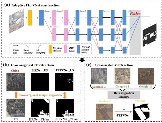
3.1. Proposal of a Filter-Embedded Neural Network
As shown in Figure 2, HRNet comprises a stem network for initial feature extraction and a multi-scale resolution main body network. The main body network contains four stages, each using residual blocks to extract features. At the end of each stage, a Transition branch is added, where the output features are downsampled by a factor of two, and the channels are expanded by a factor of two. Finally, the head uses bilinear interpolation to upsample the low-resolution feature maps and connects the completed upsample feature maps to the output predicted binarized maps.
Several modifications were made to improve the HRNet model, including adding high-low pass filtering, polarized parallel attention, and a deep separable convolution. Four different stem networks were constructed: LG_stem, which combines Laplacian and Gaussian filters, SG_stem, which combines Sobel and Gaussian filters, CG_stem, which combines Canny and Gaussian filters, and CM_stem, which combines Canny and Median filters. In addition, the Polarized Self-Attention–residual (PAR), Single Depthwise Separable (SDS) residual and Double Depthwise Separable (DDS) residual blocks were constructed to replace the standard residual blocks at different stages of the HRNet main network. The performance of these modules was evaluated on Sentinel-2 images in terms of efficiency, Precision, Recall, F1-score, and Intersection over Union (IoU) to determine the best configuration for our model.
The best-performing FEPVNet model embedded the Canny and Median filter into the stem and replaced the normal residual block in the second stage using the PAR. Considering that FEPVNet has a large number of parameters, we used an SDS block to replace the normal residual block, which dramatically reduced the number of parameters and improved the computational efficiency, and this model was named FESPVNet.
3.1.1. Stem Network Embedded Filtering
When an image is input into the HRNet model, it is initially processed by the stem network, which consists of two stride-2 3 × 3 convolutions, resulting in a feature map that is 1/4 the size of the original image. The architecture of the stem network utilized in HRNet is depicted in Figure 3a.
To enhance the stem network’s capability for an adaptive extraction of the boundary features, we constructed the high-pass filter (HPF) residual structure depicted in the left half of Figure 3b. This was achieved by using traditional computer vision methods such as Canny [40], Sobel [41], and Laplacian [42] high-pass filters. We then embedded these filters into the stem network so that the network could obtain images containing edge features. Next, we embedded low-pass filters, such as Gaussian and Median [43,44], into the stem network. as shown in the right half of Figure 3b, to filter out the noise in the feature maps. Finally, we experimented with combining the above filters and determined that it was optimal to embed the Canny and Median filters into the stem network.
The following are the steps for edge detection by Canny:
- 1.
- To perform the image smoothing, a Gaussian filter with a two-dimensional Gaussian kernel is used to carry out a convolution calculation to complete a weighted average of the image. This process is effective in filtering out the high-frequency noise in the image. The calculation process is as follows:
- 2.
- The edges are determined based on the image’s gradient amplitude and gradient direction. Here, the gradient amplitude and direction are calculated using the Sobel operator for the image with the following equation:
- 3.
- To remove the non-boundary points, non-maximum suppression is applied to the entire image. This is achieved by calculating the amplitude of each pixel point relative to the gradient direction, comparing the amplitudes of pixel points with the same gradient direction, and retaining only those with the highest amplitude in the same direction. The remaining pixel points are then eliminated.
- 4.
- To detect the edges, we employ the double threshold algorithm. We define strong and weak thresholds by setting pixel points with gradient values below the weak threshold to 0 and those exceeding the strong threshold to 255. For pixel points whose gradient values fall between the strong and weak thresholds, we keep pixel points whose eight neighborhoods are larger than the strong threshold and set them to 255, while the rest are assigned a value of 0. These points are then connected to form the object’s edges.
The edge-enhanced images obtained by the HPF still contain noise, which can affect the main body network’s feature extraction ability. However, a Median filter can mitigate this issue. The Median filter is a non-linear filtering method based on a statistical theory that can remove isolated noise while retaining the complete edge information of the image. Its principle is to replace the gray value of a point in the image with the median of the gray value of each point in the neighborhood of that point, so that the value of the pixel point in the domain is close to the actual value. The process can be summarized as follows:
- 1.
- Slide the filter window across the image, with the center of the window overlapping the position of a pixel in the image.
- 2.
- Obtain the gray value of the corresponding pixel in this window.
- 3.
- Sort the grayscale values obtained from smallest to largest and find the median value in the middle of the sorted list.
- 4.
- Assign the median value to the pixel at the window’s center.
3.1.2. The Main Body Network Adaptability Improvements
The PSA [45] mechanism adds channel attention to the self-attention mechanism based on a single spatial dimension, enabling a refined feature extraction. In this work, we use the parallel PSA, which consists of a channel branch and a spatial branch computed in parallel and then summed up, as shown in Figure 4. The calculation formula is as follows:
The Channel branch converts the input features X into Q and V using a 1 × 1 convolution. Firstly, the number of channels for Q is completely compressed to 1, and the number of channels for V becomes C/2. Since the number of channels of Q is compressed, it uses the High Dynamic Range (HDR) to enhance information by increasing the attention range for Q using the softmax function. Then Q and V are multiplied to obtain Z, and the number of Z channels is increased from C/2 to C by connecting 1 × 1 convolution and LayerNorm. Finally, the sigmoid function restricts Z between 0 and 1. The calculation formula is as follows:
The spatial branch uses a 1 × 1 convolution to convert the input features into Q and V. Global pooling is used to compress Q in the spatial dimension to a size of 1 × 1. In contrast, V’s spatial dimension remains H × W. As Q’s spatial dimension is compressed, Q’s information is augmented using softmax. The feature obtained by matrix multiplication of Q and V is reshaped 1 × H × W and converted the values to between 0 and 1 using sigmoid. The calculation formula is as follows:
The PSA minimizes information loss by avoiding significant compression in both the spatial and channel dimensions. Additionally, traditional attention methods estimate the probability using only softmax or non-linear sigmoid functions. In contrast, the PSA combines softmax and sigmoid functions in both channel and spatial branches to fit the output distribution of fine-grained regression results. Therefore, the PSA can effectively extract the features of fine-grained targets.
In this study, we use the parallel PSA to improve the basic residual convolution block construct the polarized attention residual block (PAR), and employ it in stage 2, stage 3, and stage 4 of the HRNet main body network. In addition, we experimentally determine the additional position of the PAR in each stage.
Figure 5 illustrates the normal convolution operation. By performing N 3 × 3 convolution calculations on the H × W × C feature map, an H × W × N feature map can be output. The parameters for this operation can be calculated as follows:
Howard et al. [46] proposed a decomposable convolution operation called Depthwise Separable Convolution, as shown in Figure 6. This operation splits the above normal convolution into a 3 × 3 × C depthwise convolution and n 1 × 1 × C Pointwise convolution. The following parameter quantities are calculated:
By dividing the above two Equations (9) and (10), we can obtain the following results:
From the above Equation (10), it can be observed that replacing the normal 3 × 3 convolution with the Depthwise Separable Convolution reduces the number of parameters in the replaced part by 1/8~1/9 of the original, leading to significant improvements in the computational efficiency and a lighter network. Therefore, in this study, we use the Depthwise Separable Convolution to replace the basic residual convolution block in Figure 7a, constructing two kinds of deep convolution residual blocks, as follows:
We used SDS and DDS for stage 2, stage 3, and stage 4 of the HRNet main body, respectively. Through the experiments, we found that SDS outperformed the normal residual block in stage 4.
3.2. Evaluation of the Model Adaptability
Figure 1c shows that the FEPVNet model was employed for cross-validation to verify its ability to adaptively extract PVs from different regions. Specifically, we trained the FEPVNet model with the Sentinel-2 China dataset to extract PVs from the US region and vice versa.
To enhance the generalizability of the Sentinel-2 image model in multi-source images and facilitate its migration for use in high-resolution image models, we compared four methods illustrated in Figure 1d, which include three image migration strategies. These methods consist of training the model with the Sentinel-2 dataset, mixing Sentinel-2 images with Google-14 images in a 1:1 ratio to form the dataset training model, mixing Sentinel-2 images with Google-16 images in a 1:1 ratio to form the dataset training model, and mixing Sentinel-2 images with Google-14 and Google-16 images in a 1:1:2 to form the dataset training model. We then used these methods to extract PVs from the Gaofen-2 image.
3.3. Evaluation Metrics
To evaluate the results of PV extraction, we utilized four metrics, namely Precision, Recall, F1-score, and IoU. The calculations for these metrics can be completed using the following equations:
In the above Equations (11)–(14), TP represents a positive sample judged as positive, FP represents a negative sample judged as a positive, FN represents a positive sample judged as negative, and TN represents a negative sample judged as negative.
4. Results
4.1. Ablation Experiment of Filter-Embedded Neural Network
We conducted ablation experiments using Sentinel-2 image to construct an optimal filtering embedded neural network. We tested four different stem networks and replaced normal residual blocks at various stages of the HRNet’s main body with PAR, SDS, and DDS modules to better understand the impact of each module on the model’s performance. We identified our model’s optimal configuration based on these experiments’ results.
4.1.1. The Results of Different Stem Models
The results in Table 2 show that, on the Sentinel-2 dataset, except for SG_stem, the evaluation metrics of the improved stem models are higher than those of the stem. Specifically, on the Sentinel-2 dataset in the US, CM_stem had an increase in F1-score and IoU of 0.97% and 1.80%, respectively, compared to the stem. On the Sentinel-2 dataset in China, the F1-score and IoU of CM_stem increased by 1.25% and 2.25% over the stem, respectively. However, the other improvement methods only resulted in slight improvements in the evaluation metrics compared to the stem.
Figure 8 shows the prediction results of different stem networks on the Sentinel-2 dataset in the US and China. By comparing the Ground truth and the five prediction results, it was found that the segmentation results of the CM_stem network in the last column were consistent with the labels. Compared with other models, the segmentation result of the CM_stem network in the last column was consistent with the label. As indicated by the red circle in Figure 8, other network models wrongly classified the segmentation results of the small boundary as PVs, while the segmentation results of the CM_stem network retained the edge. Combining the prediction results and evaluation metrics of the two datasets, we determined that the final method for improving the stem network is CM_stem, which embeds Canny and the Median filter in the stem, as shown in Figure 3b.
4.1.2. The Results of Models in Different Stages
Table 3 presents the evaluation metrics obtained from the ablation experiments in the main body network improvement on Sentinel-2 images in China and the US. Comparing the evaluation metrics of HRNet in Table 2, we found that replacing the residual blocks in the HRNet main body network with PAR blocks improved the PV extraction performance in the China region. In contrast, the PV extraction performance in the US region remained almost the same. Therefore, considering that using PAR blocks increases the model’s parameter count and Flops, we decided to use it in stage 2 of the main body network. In addition, by comparing the performance of two different residual blocks, namely the ordinary residual block and the SDS block, in the fourth stage of HRNet, it was observed that replacing the former with the latter can reduce 39,873,600 parameters and 122.58 G Flops without any significant change in the evaluation metrics.
As shown in Figure 9, we demonstrate the representative prediction results of the ablation experiments on optimizing the backbone network. When PAR replaces the normal residual block in stage 2 for PV extraction, the results are consistent with the labels. However, when SDS replaces the standard residual block in the fourth stage for PV extraction, some of the extracted PV results are slightly missing. Compared with other stages using PAR and SDS, the stages where the two residual blocks are replaced, have good performance. In addition, when DDS is used to replace the normal residual block in stage 4 for PV extraction, some PV panels with less salient features cannot be identified. The prediction results of this improvement method are consistent with the other residual improvement methods of the backbone network.
4.2. The Filter-Embedded Neural Network for PV Panel Mapping
Based on the ablation experiments conducted to improve HRNet’s stem and main body network, we integrated the best-performing modules of each part to build two improved models: FEPVNet and FESPVNet. FEPVNet replaces HRNet’s stem and stage 2 residual blocks in the main body network with CM_stem and PAR, respectively. FESPVNet replaces the stage 4 residual blocks in FEPVNet’s main body network with SDS. We then compared the PV extraction results of U-Net, HRNet, SwinTransformer [47], FEPVNet, and FESPVNet on Sentinel-2 images of the US and China.
Table 4 presents the evaluation metrics of different network models on Sentinel-2 images in different regions, namely China and the US. By comparing the evaluation metrics of different models, we observed that FEPVNet’s IoU increased by 2.05% in the US and 2.37% in China compared to HRNet. Furthermore, compared to HRNet, FESPVNet reduced the number of parameters by 39,780,864 and Flops by 120.74 G. However, FESPVNet’s IoU increased by 1.2% in the US and 1.89% in China.
Figure 10 shows the PV prediction results of four network models. From the content of the figure, it can be observed that U-Net has the worst prediction results, with many PV areas still unidentified. In contrast, our proposed models, especially FEPVNet, perform better than HRNet in the region marked by the red circle. Additionally, FEPVNet can segment PV boundaries that HRNet cannot.
4.3. The Adaptability of the Model under Different Regions
We trained HRNet and FEPVNet using Sentinel-2 images from various regions in China and the US. To assess the cross-regional generalizability of the models, we conducted cross-validation experiments where the trained American model was used to predict images from the China region, and the Chinese model was used to predict images from the US region. The evaluation metrics are shown in Table 5.
Comparing the cross-validation results’ evaluation metrics in Table 5 with those in Table 4, we observed that using US weights to predict the Chinese regional images resulted in a 31.25% and 43.24% decrease in the F1-score and IoU, respectively. Similarly, using Chinese weights to predict US regional images led to a 28.30% and 45.12% reduction in F1-score and IoU, respectively. Despite the decrease in metrics for cross-validation, FEPVNet demonstrated better performance than HRNet in both the US and China regions, achieving an F1-score and IoU of 3.96% and 4.24% higher in the US region and 8.86% and 8.81% higher in the Chinese region, respectively.
In Figure 11, the red dashed boxes represent the prediction result plots for cross-validation, while the remaining boxes represent the prediction result plots without cross-validation. By comparing the two types of prediction results and analyzing the label changes in the two types of evaluation metrics, we found that both HRNet and FEPVNet missed PV extraction results during cross-validation. However, FEPVNet demonstrated better PV extraction ability and a more stable performance than HRNet.
4.4. The Adaptability of the Model under Multi-Source Images
We proposed three data migration strategies to achieve cross-scale extraction of PVs. Since we used Gaofen-2 images of the China region in this study, we found the prediction results of both the HRNet and FEPVNet models were severely missing when we used a model trained on Sentinel-2 images to extract PVs from Gaofen-2 images, as shown in the third column of Figure 12. Comparing the prediction results with the evaluation metrics in Table 6 shows that the results were poor when directly using the Sentinel-2 model to extract PV from Gaofen-2 images. Therefore, we utilized three data migration strategies (i.e., using Google data as a medium for Sentinel-2 and Gaofen-2 images) to improve the accuracy of PV extraction.
The prediction results of the Sentinel-2 combined with the Google-14 image strategy are shown in the fourth column of Figure 12, the prediction results of the Sentinel-2 combined with the Google-16 image strategy are shown in the fifth column of Figure 12, and the prediction results of the Sentinel-2 and Google-14 16 combination strategy are shown in the sixth column of Figure 12. From the contents of Figure 12, we have seen that the prediction results of FEPVNet in the fifth column are consistent with the labels. According to the evaluation metrics in Table 6, the optimal cross-scale PV extraction scheme was the FEPVNet model combined with the Sentinel-2 and Google-16 combination strategy. Its prediction results of the F1-score and IoU reached 91.42% and 84.19%, respectively. In addition, the evaluation metrics of PVs extracted by FEPVNet all exceeded the evaluation metrics of HRNet in the same case.
We utilized the FEPVNet model with the optimal evaluation metrics to extract PVs from Gaofen-2 images, as illustrated in Figure 13. The red box in the circle diagram in the upper left corner of Figure 13a represents the geographic location of the Gaofen-2 image. The red area in the figure represents the extracted results of the PVs. The blue dashed box area in Figure 13a is magnified, as shown in Figure 13b, and Figure 13c shows the prediction result of Figure 13b. Combining data migration and FEPVNet can effectively extract PVs from the Gaofen-2 image.
5. Discussion
In previous studies of PV extraction, some traditional methods and un-optimized CNNs [21,22,23,24] have been used for PV extraction from a single data source, achieving good results but with poor generalization. Although Kruitwagen et al. [32] achieved PV extraction from multiple sources of images with the same resolution, cross-scale PV extraction has not been completed. Based on the deficiencies in the above research, we conducted a model of experiments using Sentinel-2 images to build FEPVNet. We combined Sentinel-2 and Google images to construct three data migration strategies to complete PV extraction from Gaofen-2 images.
Given that previous methods have difficulty extracting small features at the edge of PV panels and that image noise significantly influenced the extraction results, we embedded Canny and Median filters into the stem to construct the CM_stem. As shown in the prediction results in the last column of Figure 8, the above improvements effectively enhanced the model’s edge extraction ability and anti-noise. To enhance the adaptive capability of the model, we constructed PAR using PSA to replace the noraml residual block and determined through ablation experiments which should be used in stage 2 of the main body network, as shown in the best ablation experiment result in the third column of Figure 9. Finally, we combined the CM_stem and PAR to propose the adaptive FEPVNet. To reduce the number of parameters and improve the computational efficiency, we used the SDS module to replace the normal residual block in stage 4 of FEPVNet and named this model FESPVNet. After significantly reducing the number of model parameters, the loss of each evaluation metric was less than 0.5%, indicating that our method achieved a good balance between model accuracy and computational cost.
Furthermore, to demonstrate the adaptive capability of FEPVNet for PV extraction, we conducted cross-validation of HRNet and FEPVNet. The quantitative evaluation metrics are shown in Table 5. As the results show, the evaluation metrics of the prediction results of both models have declined. The imbalance in the number of training images available from the different regions can affect the model’s learning of photovoltaic features and its prediction of photovoltaic results, which is difficult to avoid in deep learning training completely. Under the fixed data source, appropriate over- or undersampling strategies, weight updating strategies, or weighted loss functions may be adopted to improve the adverse effects caused by this problem. In addition, the decline in evaluation indicators in cross-validation results is also affected by regional differences. For example, as shown in Figure 14, the landscapes in Chinese images are more straightforward than those in the US, and the colors of the images are also significantly different (e.g., the green PV area and the yellow circle in the figure). The difference in the data itself may require some image pre-processing or post-processing strategies to reduce the impact while also placing higher demands on the model’s generalization ability. Nevertheless, in cross-validation, the performance of FEPVNet was still superior to that of HRNet, indicating that our method has a high PV extraction accuracy and good generalization ability to cope with different regional data.
Finally, we compared the PV cross-scale extraction results of three migration strategies and two models (i.e., HRNet and FEPVNet), and the quantitative evaluation metrics are shown in Table 6. The FEPVNet model combined with the optimal migration strategy of mixing Sentinel-2 and Google-16 images can accurately extract photovoltaic information from Gaofen-2 satellite images. This study has positive implications for large-scale PV mapping and can provide accurate PV geospatial information for those who need it.
6. Conclusions
The primary purpose of this study is to propose a cross-scale PV mapping method based on the FEPVNet model, which is used to extract photovoltaic regions from multiple sources of images adaptively. For experiments, four datasets were constructed using global PV vector samples from Sentinel-2, Google-14, Google-16, and Gaofen-2.
To enhance the anti-noise edge information extraction and high-dimensional local feature extraction capabilities of the network, we embedded Canny, Median filter, and PSA into HRNet to construct the FEPVNet model. Subsequently, we conducted comparative experiments and cross-validation experiments on the Sentinel-2 dataset. The results of the comparative experiments show that compared to classical methods such as U-Net and HRNet, FEPVNet has a higher PV extraction accuracy. Furthermore, in the cross-validation experiments with different regional images, FEPVNet mitigated the impact of training data imbalance and regional differences on PV extraction compared to HRNet. Finally, we used the data migration strategies to enable the FEPVNet model trained on Sentinel-2 images to extract PVs across scales in Gaofen-2 images, with Precision and F1-score reaching 94.37% and 91.42%, respectively, which demonstrates the effectiveness of our method.
The main contribution of this study is to construct an adaptive Filter-Embedded Network (i.e., FEPVNet) and data migration strategies to accomplish the cross-scale mapping of PV panels from multi-source images. In the future, we will investigate the model’s ability to extract other types of PV, such as rooftop photovoltaics, and its applicability to other remote-sensing images. We will also use the cross-scale PV extraction method proposed in this study to complete regional or national-scale PV mapping.
Author Contributions
Conceptualization, X.D., F.C., X.L. (Xuecao Li) and X.L. (Xiaonan Luo); methodology, B.S., X.D. and H.M.; software, X.D. and X.L. (Xuecao Li); validation, B.S., H.M. and C.X.; formal analysis, B.S.; data curation, B.S. and H.M.; writing—original draft preparation, B.S. and H.M.; writing—review and editing, X.D., B.S. and H.M.; supervision, X.D., X.L. (Xuecao Li) and X.L. (Xiaonan Luo); project administration, X.D. and C.X. All authors have read and agreed to the published version of the manuscript.
Funding
This work is supported by the Strategic Priority Research Program of the Chinese Academy of Sciences, Project CASEarth (XDA19080101 and XDA19080103), the Innovation Drive Development Special Project of Guangxi (GuikeAA20302022).
Data Availability Statement
The vector files used in creating the dataset were obtained from “https://zenodo.org/record/5005868”. The dataset produced for this study is available on request to the corresponding author.
Conflicts of Interest
The authors declare no conflict of interest.
References
- BP. Statistical Review of World Energy. 2022. Available online: https://www.bp.com/en/global/corporate/energy-economics/statistical-review-of-world-energy.html (accessed on 20 October 2022).
- Chu, S.; Majumdar, A. Opportunities and challenges for a sustainable energy future. Nature 2012, 488, 294–303. [Google Scholar] [CrossRef] [PubMed]
- Kabir, E.; Kumar, P.; Kumar, S.; Adelodun, A.A.; Kim, K.-H. Solar energy: Potential and future prospects. Renew. Sustain. Energy Rev. 2018, 82, 894–900. [Google Scholar] [CrossRef]
- Dai, Z.; Liu, H.; Le, Q.V.; Tan, M. Coatnet: Marrying convolution and attention for all data sizes. Adv. Neural Inf. Process. Syst. 2021, 34, 3965–3977. [Google Scholar]
- Perez, R.; Kmiecik, M.; Herig, C.; Renné, D. Remote monitoring of PV performance using geostationary satellites. Sol. Energy 2001, 71, 255–261. [Google Scholar] [CrossRef]
- Jiang, H.; Yao, L.; Lu, N.; Qin, J.; Liu, T.; Liu, Y.; Zhou, C. Multi-resolution dataset for photovoltaic panel segmentation from satellite and aerial imagery. Earth Syst. Sci. Data 2021, 13, 5389–5401. [Google Scholar] [CrossRef]
- Niazi, K.A.K.; Akhtar, W.; Khan, H.A.; Yang, Y.; Athar, S. Hotspot diagnosis for solar photovoltaic modules using a Naive Bayes classifier. Sol. Energy 2019, 190, 34–43. [Google Scholar]
- Tsanakas, J.A.; Chrysostomou, D.; Botsaris, P.N.; Gasteratos, A. Fault diagnosis of photovoltaic modules through image processing and Canny edge detection on field thermographic measurements. Int. J. Sustain. Energy 2015, 34, 351–372. [Google Scholar] [CrossRef]
- Aghaei, M.; Leva, S.; Grimaccia, F. PV power plant inspection by image mosaicing techniques for IR real-time images. In Proceedings of the 2016 IEEE 43rd Photovoltaic Specialists Conference (PVSC), Portland, OR, USA, 5–10 June 2016; pp. 3100–3105. [Google Scholar]
- Joshi, B.; Hayk, B.; Al-Hinai, A.; Woon, W.L. Rooftop detection for planning of solar PV deployment: A case study in Abu Dhabi. In Proceedings of the Data Analytics for Renewable Energy Integration: Second ECML PKDD Workshop, DARE 2014, Nancy, France, 19 September 2014; pp. 137–149. [Google Scholar]
- Jiang, M.; Lv, Y.; Wang, T.; Sun, Z.; Liu, J.; Yu, X.; Yan, J. Performance analysis of a photovoltaics aided coal-fired power plant. Energy Procedia 2019, 158, 1348–1353. [Google Scholar] [CrossRef]
- Ji, S.; Zhang, Z.; Zhang, C.; Wei, S.; Lu, M.; Duan, Y. Learning discriminative spatiotemporal features for precise crop classification from multi-temporal satellite images. Int. J. Remote Sens. 2020, 41, 3162–3174. [Google Scholar] [CrossRef]
- Wang, M.; Cui, Q.; Sun, Y.; Wang, Q. Photovoltaic panel extraction from very high-resolution aerial imagery using region–line primitive association analysis and template matching. ISPRS J. Photogramm. Remote Sens. 2018, 141, 100–111. [Google Scholar] [CrossRef]
- Sahu, A.; Yadav, N.; Sudhakar, K. Floating photovoltaic power plant: A review. Renew. Sustain. Energy Rev. 2016, 66, 815–824. [Google Scholar] [CrossRef]
- Al Garni, H.Z.; Awasthi, A. Solar PV power plant site selection using a GIS-AHP based approach with application in Saudi Arabia. Appl. Energy 2017, 206, 1225–1240. [Google Scholar] [CrossRef]
- Hammoud, M.; Shokr, B.; Assi, A.; Hallal, J.; Khoury, P. Effect of dust cleaning on the enhancement of the power generation of a coastal PV-power plant at Zahrani Lebanon. Sol. Energy 2019, 184, 195–201. [Google Scholar] [CrossRef]
- Zhang, X.; Xu, M.; Wang, S.; Huang, Y.; Xie, Z. Mapping photovoltaic power plants in China using Landsat, random forest, and Google Earth Engine. Earth Syst. Sci. Data 2022, 14, 3743–3755. [Google Scholar] [CrossRef]
- Du, P.; Bai, X.; Tan, K.; Xue, Z.; Samat, A.; Xia, J.; Li, E.; Su, H.; Liu, W. Advances of Four Machine Learning Methods for Spatial Data Handling: A Review. J. Geovis. Spat. Anal. 2020, 4, 13. [Google Scholar] [CrossRef]
- Gao, X.; Wu, M.; Li, C.; Niu, Z.; Chen, F.; Huang, W. Influence of China’s Overseas power stations on the electricity status of their host countries. Int. J. Digit. Earth 2022, 15, 416–436. [Google Scholar] [CrossRef]
- Li, E.; Xia, J.; Du, P.; Lin, C.; Samat, A. Integrating Multilayer Features of Convolutional Neural Networks for Remote Sensing Scene Classification. IEEE Trans. Geosci. Remote Sens. 2017, 55, 5653–5665. [Google Scholar] [CrossRef]
- Huang, H.; Huang, J.; Feng, Q.; Liu, J.; Li, X.; Wang, X.; Niu, Q. Developing a Dual-Stream Deep-Learning Neural Network Model for Improving County-Level Winter Wheat Yield Estimates in China. Remote Sens. 2022, 14, 5280. [Google Scholar] [CrossRef]
- Samat, A.; Li, E.; Wang, W.; Liu, S.; Liu, X. HOLP-DF: HOLP Based Screening Ultrahigh Dimensional Subfeatures in Deep Forest for Remote Sensing Image Classification. IEEE J. Sel. Top. Appl. Earth Obs. Remote Sens. 2022, 15, 8287–8298. [Google Scholar] [CrossRef]
- Tang, W.; Yang, Q.; Xiong, K.; Yan, W. Deep learning based automatic defect identification of photovoltaic module using electroluminescence images. Sol. Energy 2020, 201, 453–460. [Google Scholar] [CrossRef]
- Deitsch, S.; Christlein, V.; Berger, S.; Buerhop-Lutz, C.; Maier, A.; Gallwitz, F.; Riess, C. Automatic classification of defective photovoltaic module cells in electroluminescence images. Sol. Energy 2019, 185, 455–468. [Google Scholar] [CrossRef]
- Li, X.; Yang, Q.; Lou, Z.; Yan, W. Deep learning based module defect analysis for large-scale photovoltaic farms. IEEE Trans. Energy Convers. 2018, 34, 520–529. [Google Scholar] [CrossRef]
- Malof, J.M.; Rui, H.; Collins, L.M.; Bradbury, K.; Newell, R. Automatic solar photovoltaic panel detection in satellite imagery. In Proceedings of the 2015 International Conference on Renewable Energy Research and Applications (ICRERA), Palermo, Italy, 22–25 November 2015; pp. 1428–1431. [Google Scholar]
- Yuan, J.; Yang, H.H.L.; Omitaomu, O.A.; Bhaduri, B.L. Large-scale solar panel mapping from aerial images using deep convolutional networks. In Proceedings of the 2016 IEEE International Conference on Big Data (Big Data), Washington, DC, USA, 5–8 December 2016; pp. 2703–2708. [Google Scholar]
- Jumaboev, S.; Jurakuziev, D.; Lee, M. Photovoltaics plant fault detection using deep learning techniques. Remote Sens. 2022, 14, 3728. [Google Scholar] [CrossRef]
- Xu, C.; Du, X.; Fan, X.; Giuliani, G.; Hu, Z.; Wang, W.; Liu, J.; Wang, T.; Yan, Z.; Zhu, J.; et al. Cloud-based storage and computing for remote sensing big data: A technical review. Int. J. Digit. Earth 2022, 15, 1417–1445. [Google Scholar] [CrossRef]
- Xu, C.; Du, X.; Jian, H.; Dong, Y.; Qin, W.; Mu, H.; Yan, Z.; Zhu, J.; Fan, X. Analyzing large-scale Data Cubes with user-defined algorithms: A cloud-native approach. Int. J. Appl. Earth Obs. Geoinf. 2022, 109, 102784. [Google Scholar] [CrossRef]
- Qi, Z.; Xuelong, L. Big data: New methods and ideas in geological scientific research. Big Earth Data 2019, 3, 1–7. [Google Scholar] [CrossRef]
- Kruitwagen, L.; Story, K.T.; Friedrich, J.; Byers, L.; Skillman, S.; Hepburn, C. A global inventory of photovoltaic solar energy generating units. Nature 2021, 598, 604–610. [Google Scholar] [CrossRef]
- Yu, J.; Wang, Z.; Majumdar, A.; Rajagopal, R. DeepSolar: A Machine Learning Framework to Efficiently Construct a Solar Deployment Database in the United States. Joule 2018, 2, 2605–2617. [Google Scholar] [CrossRef]
- Xia, Z.; Li, Y.; Guo, X.; Chen, R. High-resolution mapping of water photovoltaic development in China through satellite imagery. Int. J. Appl. Earth Obs. Geoinf. 2022, 107, 102707. [Google Scholar] [CrossRef]
- Zhang, W.; Du, P.; Fu, P.; Zhang, P.; Tang, P.; Zheng, H.; Meng, Y.; Li, E. Attention-Aware Dynamic Self-Aggregation Network for Satellite Image Time Series Classification. IEEE Trans. Geosci. Remote Sens. 2022, 60, 1–17. [Google Scholar] [CrossRef]
- Tang, P.; Du, P.; Xia, J.; Zhang, P.; Zhang, W. Channel Attention-Based Temporal Convolutional Network for Satellite Image Time Series Classification. IEEE Geosci. Remote Sens. Lett. 2022, 19, 1–5. [Google Scholar] [CrossRef]
- Zhu, S.; Du, B.; Zhang, L.; Li, X. Attention-based multiscale residual adaptation network for cross-scene classification. IEEE Trans. Geosci. Remote Sens. 2021, 60, 1–15. [Google Scholar] [CrossRef]
- Sun, K.; Zhao, Y.; Jiang, B.; Cheng, T.; Xiao, B.; Liu, D.; Mu, Y.; Wang, X.; Liu, W.; Wang, J. High-resolution representations for labeling pixels and regions. arXiv 2019, arXiv:1904.04514. [Google Scholar]
- Wang, J.; Sun, K.; Cheng, T.; Jiang, B.; Deng, C.; Zhao, Y.; Liu, D.; Mu, Y.; Tan, M.; Wang, X.; et al. Deep High-Resolution Representation Learning for Visual Recognition. IEEE Trans. Pattern Anal. Mach. Intell. 2021, 43, 3349–3364. [Google Scholar] [CrossRef]
- Canny, J. A Computational Approach to Edge Detection. IEEE Trans. Pattern Anal. Mach. Intell. 1986, PAMI-8, 679–698. [Google Scholar] [CrossRef]
- Kanopoulos, N.; Vasanthavada, N.; Baker, R.L. Design of an image edge detection filter using the Sobel operator. IEEE J. Solid-State Circuits 1988, 23, 358–367. [Google Scholar] [CrossRef]
- Wang, X. Laplacian Operator-Based Edge Detectors. IEEE Trans. Pattern Anal. Mach. Intell. 2007, 29, 886–890. [Google Scholar] [CrossRef] [PubMed]
- Huber, M.F.; Hanebeck, U.D. Gaussian Filter based on Deterministic Sampling for High Quality Nonlinear Estimation. IFAC Proc. Vol. 2008, 41, 13527–13532. [Google Scholar] [CrossRef]
- Kumar, A.; Sodhi, S.S. Comparative Analysis of Gaussian Filter, Median Filter and Denoise Autoenocoder. In Proceedings of the 2020 7th International Conference on Computing for Sustainable Global Development (INDIACom), New Delhi, India, 12–14 March 2020; pp. 45–51. [Google Scholar]
- Liu, H.; Liu, F.; Fan, X.; Huang, D. Polarized self-attention: Towards high-quality pixel-wise mapping. Neurocomputing 2022, 506, 158–167. [Google Scholar] [CrossRef]
- Howard, A.G.; Zhu, M.; Chen, B.; Kalenichenko, D.; Wang, W.; Weyand, T.; Andreetto, M.; Adam, H. MobileNets: Efficient Convolutional Neural Networks for Mobile Vision Applications. arXiv 2017, arXiv:1704.04861. [Google Scholar]
- Liu, Z.; Lin, Y.; Cao, Y.; Hu, H.; Wei, Y.; Zhang, Z.; Lin, S.; Guo, B. Swin transformer: Hierarchical vision transformer using shifted windows. In Proceedings of the IEEE/CVF International Conference on Computer Vision, Montreal, BC, Canada, 11–17 October 2021; pp. 10012–10022. [Google Scholar]
Figure 1.
Illustration of the method framework. (a) PV dataset preparation workflow, (b) ablation experiment of FEPVNet workflow, (c) different models of PV panel extraction from Sentinel-2 images, (d) FEPVNet cross-validation, (e) multi-source images to complete cross-scale PV extraction.
Figure 1.
Illustration of the method framework. (a) PV dataset preparation workflow, (b) ablation experiment of FEPVNet workflow, (c) different models of PV panel extraction from Sentinel-2 images, (d) FEPVNet cross-validation, (e) multi-source images to complete cross-scale PV extraction.

Figure 2.
The FEPVNet model structure.

Figure 3.
Comparison of the stem network improvements. (a) HRNet stem network, (b) improved HRNet stem network.
Figure 3.
Comparison of the stem network improvements. (a) HRNet stem network, (b) improved HRNet stem network.

Figure 4.
Parallel Polarized Self-Attention.

Figure 5.
Normal convolution operation.

Figure 6.
The Depthwise Separable Convolution operation.

Figure 7.
Four residual structures. (a) Normal residual block, (b) Polarized Self-Attention–residual block, (c) Single Depthwise Separable residual block, (d) Double Depthwise Separable residual block.
Figure 7.
Four residual structures. (a) Normal residual block, (b) Polarized Self-Attention–residual block, (c) Single Depthwise Separable residual block, (d) Double Depthwise Separable residual block.

Figure 8.
The predicted results for different stem networks in China and the US. Note: For the adaptation improvement of stem networks, we complete five stem network comparison experiments: original stem, LG_stem combined with Laplacian and Gaussian, SG_stem combined with Sobel and Gaussian, CG_stem combined with Canny and Gaussian, and CM_stem combined with Canny and Median.

Figure 9.
The prediction results for China and the US in different stages of network models. Note: The prediction results of stages using PAR, DDS, and SDS improvement in China and US regions are shown.
Figure 9.
The prediction results for China and the US in different stages of network models. Note: The prediction results of stages using PAR, DDS, and SDS improvement in China and US regions are shown.

Figure 10.
The prediction results for China and the US in different network models. Note: The prediction results of U-Net, HRNet, SwinTransformer, FESPVNet, and FEPVNet in China and US regions are shown.
Figure 10.
The prediction results for China and the US in different network models. Note: The prediction results of U-Net, HRNet, SwinTransformer, FESPVNet, and FEPVNet in China and US regions are shown.

Figure 11.
Cross-validation results. Note: The prediction results of HRNet and FEPVNet for China and US regions with different weight parameters are shown.
Figure 11.
Cross-validation results. Note: The prediction results of HRNet and FEPVNet for China and US regions with different weight parameters are shown.

Figure 12.
The prediction results of two models with different data migration strategies. Note: The prediction results of HRNet and FEPVNet models are shown for four migration strategies for the Gaofen data.
Figure 12.
The prediction results of two models with different data migration strategies. Note: The prediction results of HRNet and FEPVNet models are shown for four migration strategies for the Gaofen data.

Figure 13.
The best prediction results for Gaofen-2 image region. (a) PV mapping on the Gaofen-2 image, (b) the original Gaofen-2 image in the blue box in (a), (c) PV mapping results in the blue box in (a), and PVs in the red area. Note: Complete PV mapping on the Gaofen-2 image using the model with the best evaluation metrics.

Figure 14.
Data presentation of the US region and China region.


Table 1.
The dataset properties.
| Dataset Name | Resolution | Region | Number of Training Sets | Number of Validation Sets | Number of Test Sets |
|---|---|---|---|---|---|
| Sentinel-2 | 10 m | China | 1037 | 49 | 177 |
| Sentinel-2 | 10 m | US | 426 | 51 | 98 |
| Google-14 | 10 m | China | 1000 | 0 | 0 |
| Google-16 | 2 m | China | 1000 | 0 | 0 |
| Gaofen-2 | 2 m | China | 0 | 52 | 118 |
Table 2.
The evaluation metrics for different stem networks in China and the US.
| Region | Model | Recall | Precision | F1-Score | IoU |
|---|---|---|---|---|---|
| China | stem | 0.9052 | 0.9489 | 0.9265 | 0.8631 |
| LG_stem | 0.8965 | 0.9336 | 0.9147 | 0.8428 | |
| SG_stem | 0.8830 | 0.9057 | 0.8942 | 0.8087 | |
| CG_stem | 0.9065 | 0.9226 | 0.9145 | 0.8425 | |
| CM_stem | 0.9315 | 0.9472 | 0.9393 | 0.8856 | |
| US | stem | 0.9521 | 0.9595 | 0.9558 | 0.9153 |
| LG_stem | 0.9498 | 0.9564 | 0.9531 | 0.9105 | |
| SG_stem | 0.9444 | 0.9443 | 0.9444 | 0.8946 | |
| CG_stem | 0.9541 | 0.9700 | 0.9620 | 0.9268 | |
| CM_stem | 0.9619 | 0.9691 | 0.9655 | 0.9333 |
Table 3.
The evaluation metrics for different main body networks.
| Region | Model | Recall | Precision | F1-Score | IoU | Params | Flops |
|---|---|---|---|---|---|---|---|
| China | PAR_stage2 | 0.9306 | 0.9423 | 0.9364 | 0.8805 | 65,939,858 | 376.34 G |
| PAR_stage3 | 0.9241 | 0.9372 | 0.9306 | 0.8702 | 67,400,786 | 385.47 G | |
| PAR_stage4 | 0.9281 | 0.9481 | 0.9380 | 0.8833 | 70,555,922 | 385.45 G | |
| DDS_stage2 | 0.9202 | 0.9369 | 0.9285 | 0.8665 | 65,120,210 | 355.52 G | |
| DDS_stage3 | 0.9247 | 0.9149 | 0.9198 | 0.8515 | 53,557,586 | 260.13 G | |
| DDS_stage4 | 0.9217 | 0.9265 | 0.9241 | 0.8590 | 28,401,362 | 259.82 G | |
| SDS_stage2 | 0.9215 | 0.9366 | 0.9290 | 0.8675 | 65,068,946 | 354.14 G | |
| SDS_stage3 | 0.9147 | 0.9388 | 0.9266 | 0.8633 | 52,735,058 | 252.09 G | |
| SDS_stage4 | 0.9277 | 0.9380 | 0.9328 | 0.8742 | 25,973,522 | 251.93 G | |
| US | PAR_stage2 | 0.9422 | 0.9655 | 0.9537 | 0.9116 | 65,939,858 | 376.34 G |
| PAR_stage3 | 0.9318 | 0.9605 | 0.9459 | 0.8975 | 67,400,786 | 385.47 G | |
| PAR_stage4 | 0.9467 | 0.9615 | 0.9540 | 0.9122 | 70,555,922 | 385.45 G | |
| DDS_stage2 | 0.9409 | 0.9650 | 0.9528 | 0.9099 | 65,120,210 | 355.52 G | |
| DDS_stage3 | 0.9361 | 0.9617 | 0.9487 | 0.9025 | 53,557,586 | 260.13 G | |
| DDS_stage4 | 0.9410 | 0.9582 | 0.9495 | 0.9039 | 28,401,362 | 259.82 G | |
| SDS_stage2 | 0.9439 | 0.9609 | 0.9523 | 0.9090 | 65,068,946 | 354.14 G | |
| SDS_stage3 | 0.9417 | 0.9690 | 0.9552 | 0.9142 | 52,735,058 | 252.09 G | |
| SDS_stage4 | 0.9412 | 0.9633 | 0.9521 | 0.9087 | 25,973,522 | 251.93 G |
Table 4.
The evaluation metrics for different network models.
| Region | Model | Recall | Precision | F1-Score | IoU | Params | Flops |
|---|---|---|---|---|---|---|---|
| China | U-Net | 0.4174 | 0.5316 | 0.4676 | 0.3052 | 31,054,344 | 64,914,029 |
| HRNet | 0.9052 | 0.9489 | 0.9265 | 0.8631 | 65,847,122 | 374.51 G | |
| FEPVNet | 0.9309 | 0.9493 | 0.9400 | 0.8868 | 65,939,858 | 376.34 G | |
| SwinTransformer | 0.9309 | 0.9460 | 0.9384 | 0.8840 | 59,830,000 | 936.71 G | |
| FESPVNet | 0.9246 | 0.9503 | 0.9373 | 0.8820 | 26,066,258 | 253.77 G | |
| US | U-Net | 0.8717 | 0.6224 | 0.7262 | 0.5702 | 31,054,344 | 64,914,029 |
| HRNet | 0.9521 | 0.9595 | 0.9558 | 0.9153 | 65,847,122 | 374.51 G | |
| FEPVNet | 0.9641 | 0.9695 | 0.9668 | 0.9358 | 65,939,858 | 376.34 G | |
| SwinTransformer | 0.9591 | 0.9726 | 0.9658 | 0.9339 | 59,830,000 | 936.71 G | |
| FESPVNet | 0.9567 | 0.9679 | 0.9623 | 0.9273 | 26,066,258 | 253.77 G |
Table 5.
The area comparison predictive evaluation metrics.
| Region | Model | Recall | Precision | F1-Score | IoU |
|---|---|---|---|---|---|
| China | HRNet_US | 0.3755 | 0.9372 | 0.5362 | 0.3663 |
| FEPVNet_US | 0.4645 | 0.9539 | 0.6248 | 0.4544 | |
| US | HRNet_China | 0.8288 | 0.4869 | 0.6134 | 0.4424 |
| FEPVNet_China | 0.6872 | 0.6221 | 0.6530 | 0.4848 |
Table 6.
The evaluation metrics for the model migration prediction results.
| Model | Strategy | Recall | Precision | F1-Score | IoU |
|---|---|---|---|---|---|
| HRNet | Sentinel-2 | 0.2620 | 0.9216 | 0.4084 | 0.2563 |
| Sentinel-2 Google-14 | 0.3346 | 0.9036 | 0.4884 | 0.3231 | |
| Sentinel-2 Google-16 | 0.8940 | 0.9162 | 0.9050 | 0.8265 | |
| Sentinel-2 Google-14 16 | 0.8889 | 0.9269 | 0.9075 | 0.8308 | |
| FEPVNet | Sentinel-2 | 0.2883 | 0.9083 | 0.4377 | 0.2801 |
| Sentinel-2 Google-14 | 0.6681 | 0.8724 | 0.7567 | 0.6086 | |
| Sentinel-2 Google-16 | 0.8864 | 0.9437 | 0.9142 | 0.8419 | |
| Sentinel-2 Google-14 16 | 0.9084 | 0.9192 | 0.9138 | 0.8413 |
Disclaimer/Publisher’s Note: The statements, opinions and data contained in all publications are solely those of the individual author(s) and contributor(s) and not of MDPI and/or the editor(s). MDPI and/or the editor(s) disclaim responsibility for any injury to people or property resulting from any ideas, methods, instructions or products referred to in the content. |
© 2023 by the authors. Licensee MDPI, Basel, Switzerland. This article is an open access article distributed under the terms and conditions of the Creative Commons Attribution (CC BY) license (https://creativecommons.org/licenses/by/4.0/).
Share and Cite
MDPI and ACS Style
Su, B.; Du, X.; Mu, H.; Xu, C.; Li, X.; Chen, F.; Luo, X. FEPVNet: A Network with Adaptive Strategies for Cross-Scale Mapping of Photovoltaic Panels from Multi-Source Images. Remote Sens. 2023, 15, 2469. https://doi.org/10.3390/rs15092469
AMA Style
Su B, Du X, Mu H, Xu C, Li X, Chen F, Luo X. FEPVNet: A Network with Adaptive Strategies for Cross-Scale Mapping of Photovoltaic Panels from Multi-Source Images. Remote Sensing. 2023; 15(9):2469. https://doi.org/10.3390/rs15092469
Chicago/Turabian StyleSu, Buyu, Xiaoping Du, Haowei Mu, Chen Xu, Xuecao Li, Fang Chen, and Xiaonan Luo. 2023. "FEPVNet: A Network with Adaptive Strategies for Cross-Scale Mapping of Photovoltaic Panels from Multi-Source Images" Remote Sensing 15, no. 9: 2469. https://doi.org/10.3390/rs15092469
Note that from the first issue of 2016, this journal uses article numbers instead of page numbers. See further details here.