SSANet: An Adaptive Spectral–Spatial Attention Autoencoder Network for Hyperspectral Unmixing

Abstract

Convolutional neural-network-based autoencoders, which can integrate the spatial correlation between pixels well, have been broadly used for hyperspectral unmixing and obtained excellent performance. Nevertheless, these methods are hindered in their performance by the fact that they treat all spectral bands and spatial information equally in the unmixing procedure. In this article, we propose an adaptive spectral–spatial attention autoencoder network, called SSANet, to solve the mixing pixel problem of the hyperspectral image. First, we design an adaptive spectral–spatial attention module, which refines spectral–spatial features by sequentially superimposing the spectral attention module and spatial attention module. The spectral attention module is built to select useful spectral bands, and the spatial attention module is designed to filter spatial information. Second, SSANet exploits the geometric properties of endmembers in the hyperspectral image while considering abundance sparsity. We significantly improve the endmember and abundance results by introducing minimum volume and sparsity regularization terms into the loss function. We evaluate the proposed SSANet on one synthetic dataset and four real hyperspectral scenes, i.e., Samson, Jasper Ridge, Houston, and Urban. The results indicate that the proposed SSANet achieved competitive unmixing results compared with several conventional and advanced unmixing approaches with respect to the root mean square error and spectral angle distance.

1. Introduction

Hyperspectral image (HSI) analysis has attracted a large amount of attention in the domain of remote sensing because of the rich content information contained in HSI [1,2]. Despite this, because of the inadequate spatial resolution of satellite sensors, atmospheric mixed effects, and complex ground targets, a pixel in an HSI typically includes multiple spectral features. Such pixels are known as “mixed pixels”. The presence of a large quantity of mixed pixels causes serious issues for further research on HSI [3,4,5]. Hyperspectral unmixing (HU) aims to separate the mixed pixels into a set of pure spectral signatures (endmembers) and relative mixing coefficients (abundances) [6,7,8].

Recently, with its impressive learning ability and data fitting capability, deep learning (DL) has undergone rapid development in the HU domain [9,10]. The autoencoder (AE), which is a typical representation of unsupervised DL, has been extensively applied to HU tasks. The AE framework is mainly divided into two parts: the encoder, which aims to automatically learn the low-dimensional embeddings (i.e., abundances) of input pixels, and the decoder, which aims to reconstruct input pixels with the associated basis (i.e., endmembers) [11,12]. Moreover, to achieve satisfying unmixing performance, numerous refinements have been made to the existing AE-based unmixing framework. For example, Qu and Qi [13] developed a sparse denoising AE unmixing network that introduces denoising constraints and sparsity constraints to the encoder and decoder, respectively. Zhao et al. [14] presented an AE network that uses two constraints to optimize the spectral unmixing task. Min et al. [12] designed a joint metric AE framework, which uses the Wasserstein distance and feature matching as constraints in the objective function. Jin et al. [15] designed a two-stream AE architecture, which introduces a stream to solve the problem of lacking effective guidance for the endmembers. A deep matrix factorization model was developed in [16], which constructs a multilayer nonlinear structure and employs a self-supervised constraint. Ozkan et al. [17] proposed a two-staged AE architecture that combines spectral angle distance (SAD) with multiple regularizers as the final objective. Su et al. adopted stacked AEs to handle outliers and noise, and employed a variational AE to pose the proper constraint on abundances. An end-to-end unmixing framework was proposed in [18,19], which combines the benefits of learning-based and model-based approaches. However, these methods, which receive one mixed pixel at a time during training, only use the spectral information in an HSI, thereby ignoring the spatial correlation between neighboring pixels.

Importantly, an HSI contains both rich spectral feature information and a degree of spatial information [6]. Incorporating spatial correlation in the unmixing process has been confirmed to significantly improve unmixing performance [20,21]. Therefore, many researchers have introduced convolutional neural networks (CNN) into the traditional AE structure to compensate for the absence of spatial features. For instance, Hong et al. [22] proposed a self-supervised spatial–spectral unmixing method, which incorporates an extra sub-network to guide the endmember information to obtain good unmixing results. Gao et al. [23] developed a cycle-consistency unmixing architecture and designed a self-perception loss to refine the detailed information. Rasti et al. [24] proposed a minimum simplex CNN unmixing approach that incorporates the spatial contextual structure and exploits the geometric properties of endmembers. Ayed et al. [25] presented an approach that uses extended morphological profiles, which combines the spatial correlation between pixels. In [26], a Bayesian fully convolutional framework was developed, which considers the noise, endmembers, and spatial information. Most recently, a perceptual loss-constrained adversarial AE was designed in [27], which takes into account factors such as reconstruction errors and spatial information. Hadi et al. [28] presented a hybrid 3-D and 2-D architecture to leverage the spectral and spatial features. A dual branch AE framework was constructed in [29] to incorporate spatial–contextual information.

Although the above CNN-based AE achieves satisfactory unmixing results, how to adaptively adjust the weights of spectral and spatial features that influence the unmixing performance is a new challenge. Humans can distribute their finite resources to the parts that are most significant, informative, or salient. Inspired by visual attention mechanisms, we propose a spectral–spatial attention AE network for HU and introduce a spectral–spatial attention module (SSAM) to strengthen useful information and suppress information that is unnecessary. Additionally, the absence of both abundance sparsity and endmember geometric information are also responsible for limiting unmixing performance. Thus, we combine a minimum volume constraint and sparsity constraint in the loss function. Specifically, the primary contributions of our proposed SSANet are as follows:

• We design an unsupervised unmixing network, which is based on a combination of a learnable SSAM and convolutional AE. The SSAM plays two roles. First, the spectral attention module (SEAM) adaptively learns the weights of spectral bands in input data to enhance the representation of spectral information. Second, the spatial attention module (SAAM) adaptively yields the attention weight assigned to each adjacent pixel to derive useful spatial information.
• We combine the prior knowledge that two regularizers (minimum volume regularization and sparsity regularization) are applied to endmembers and abundances, respectively. Additionally, to acquire high-quality endmember spectra, we design a new minimum volume constraint.
• We apply the proposed unmixing network to one synthetic dataset and four real hyperspectral scenes—i.e., Samson, Jasper Ridge, Houston, and Urban—and compare it with several classical and advanced approaches. Furthermore, we investigate the performance gain of SSANet with ablation experiments, involving the objective functions and network modules.

The remainder of this paper is structured as follows: In Section 2, we describe the theoretical knowledge of the AE-based unmixing approach simply. In Section 3, we explain the SSANet method in detail. In Section 4, we evaluate SSANet using synthetic and real datasets. In Section 5, we summarize the study.

2. AE-Based Unmixing Model

In the linear mixing model (LMM) [30], the observed spectral reflectance can be given by

$$\mathit{Y}=\mathit{E}\mathit{A}+\mathit{N}$$

(1)

where $\mathit{Y}=\left\{{\mathit{y}}_i|i=\mathrm{1,2},...,P\right\}\in {\mathbb{R}}^{B\times P}$ denotes the observed HSI with $B$ bands and $P$ pixels, and ${\mathit{y}}_i$ denotes the ith pixel. $\mathit{N}\in {\mathbb{R}}^{B\times P}$ denotes an additive noise matrix. $\mathit{E}=\left\{{\mathit{e}}_k|k=\mathrm{1,2},...,R\right\}\in {\mathbb{R}}^{B\times R}$ denotes the endmember matrix with $R$ endmember signatures and needs to satisfy the nonnegative constraint. $\mathit{A}=\left\{{\mathit{a}}_i|i=\mathrm{1,2},...,P\right\}\in {\mathbb{R}}^{R\times P}$ is the corresponding abundance matrix, where ${\mathit{a}}_i$ denotes the abundance percentage of the ith pixel, and should be subjected to the abundance nonnegative constraint (ANC) and abundance sum-to-one constraint (ASC)—that is,

$$\left\{\begin{array}{c}{\mathit{a}}_i\ge 0\\ {\displaystyle \sum _{k=1}^R}{\mathit{a}}_{ki}=1\end{array}\right.$$

(2)

The fundamental workflow of classic AE unmixing is shown in Figure 1 and is mainly divided into two parts.

(1) An encoder $En(·)$ transforms the input data ${\left\{{\mathit{y}}_i\right\}}_{i=1}^P\in {\mathbb{R}}^B$ into a hidden representation ${\mathit{h}}_i$, which can be described as

$${\mathit{h}}_i=En({\mathit{y}}_i)=f({\mathit{W}}^{\left(e\right)T}{y}_i+{\mathit{b}}^{\left(e\right)})$$

(3)

where ${\mathit{W}}^{\left(e\right)}$ and ${\mathit{b}}^{\left(e\right)}$ denote the weight and bias of the eth encoder layer, respectively. $f(·)$ denotes the nonlinear activation function.

(2) A decoder $De(·)$ reconstructs the data ${\left\{{\widehat{\mathit{y}}}_i\right\}}_{i=1}^P\in {\mathbb{R}}^B$ using ${\mathit{h}}_i$, which is formalized as

$${\widehat{\mathit{y}}}_i=De({\mathit{h}}_i)=W^{\left(d\right)T}{\mathit{h}}_i$$

(4)

where ${\mathit{W}}^{\left(d\right)}$ is a matrix that denotes the weights of the hidden and output layers.

Because of the characteristic of Equation (4), the output of the $En(·)$ result is considered as the predicted abundance vector, that is, ${\widehat{\mathit{a}}}_i\leftarrow {\mathit{h}}_i$, and the estimated endmember is represented by the weights of $De(·)$, that is, $\widehat{\mathit{E}}\leftarrow {\mathit{W}}^{\left(d\right)}$. In this framework, the reconstruction loss of the training process is mathematically formulated as

$${Loss}_{AE}=\frac{1}{P}\underset{i=1}{\sum ^P}{‖{\widehat{\mathit{y}}}_i-{\mathit{y}}_i‖}^2$$

(5)

3. Spectral–Spatial Attention Unmixing Network

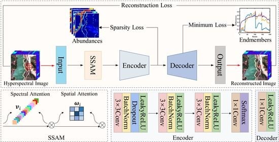
To leverage the spectral and spatial information in HSI, we first divide the HSI $\mathit{Y}$ into a set of 3-D neighboring patches $\mathit{M}=\left\{{\mathit{m}}_i|i=\mathrm{1,2},...,P\right\}\in {\mathbb{R}}^{s\times s\times B}$, where $s$ is the width of patches. In SSANet, each patch ${\mathit{m}}_i$ in $\mathit{M}$ is fed into the proposed network. In each patch ${\mathit{m}}_i$, the central pixel ${\mathit{y}}_i$ is the target pixel to be unmixed. The framework of SSANet is shown in Figure 2. Its structure consists of three core components: the SSAM, encoder, and decoder. The SSAM, which aims to provide meaningful spectral–spatial priors, helps to solidify feature extraction at later stages. The encoder is designed to extract features and reduce dimensionality. The role of the decoder is to reconstruct the learned features according to the LMM. We provide details on the aforementioned components in Section 3.1, Section 3.2, and Section 3.3, respectively.

3.1. Spectral–Spatial Attention Module

The SSAM contains two core modules—that is, the SEAM and SAAM—which are arranged sequentially to perform the selection of spectral bands and spatial features in the HSI, respectively. We describe the SEAM and SAAM in the following.

3.1.1. Spectral Attention Module

The SEAM [31] is introduced into the SSANet, aiming to adaptively learn the weights of spectral bands in the HSI in an end-to-end manner. It generates a spectral weight vector that reflects the significance of different spectral bands. The spectral bands modulated by this vector can significantly improve unmixing performance. The framework of the SEAM is shown in Figure 3.

Given the input ${\mathit{m}}_i\in {\mathbb{R}}^{s\times s\times B}$, first, global max pooling (GMP) and global average pooling (GAP) are used to acquire spectral feature vectors ${\mathit{\alpha }}_i\in {\mathbb{R}}^{1\times 1\times B}$ and ${\mathit{\beta }}_i\in {\mathbb{R}}^{1\times 1\times B}$, respectively. Next, the corresponding weight vectors ${\mathit{\gamma }}_i\in {\mathbb{R}}^{1\times 1\times B}$ and ${\mathit{\delta }}_i\in {\mathbb{R}}^{1\times 1\times B}$ can be derived using a multilayer perceptron (MLP) that can extract the weight information of each band. ${\mathit{\gamma }}_i$ and ${\mathit{\delta }}_i$ are then summed, and the sigmoid function is applied to obtain the spectral weight coefficients ${\mathit{v}}_i\in {\mathbb{R}}^{1\times 1\times B}$. The spectral attention formulation can be defined as

$${\mathit{v}}_i=\sigma \left(MLP\left(GMP\left({\mathit{m}}_i\right)\right)+MLP\left(GAP\left({\mathit{m}}_i\right)\right)\right)$$

(6)

where $\sigma (·)$ denotes the sigmoid function. Finally, the output of SEAM ${\mathit{m}}_i^{\prime }$ is calculated by the following equation:

$${\mathit{m}}_i^{\prime }={\mathit{v}}_i⨂{\mathit{m}}_i$$

(7)

3.1.2. Spatial Attention Module

In this part, we design the SAAM to evaluate the adjacent dependence between pixels. Similar to the SEAM, the SAAM also learns in an end-to-end manner and adaptively selects spatial features from the pixels in the neighborhood. The module generates a spatial weight matrix that expresses the importance of adjacent pixels. The recalibration of spatial features using this matrix leads to an obvious improvement in the unmixing accuracy. The framework of the SAAM is shown in Figure 4.

Specifically, given the input ${\mathit{m}}_i^{\prime }\in {\mathbb{R}}^{s\times s\times B}$, in order to facilitate the calculation of the similarity between neighboring pixels and the central pixel, the input ${\mathit{m}}_i^{\prime }$ is reshaped into ${\mathit{g}}_i\in {\mathbb{R}}^{ss\times B}(ss=s\times s)$. The center pixel ${\mathit{g}}_{center}\in {\mathbb{R}}^{1\times 1\times B}$ is extracted from the center of ${\mathit{m}}_i^{\mathit{\prime }}$; then, ${\mathit{g}}_{center}$ is reshaped into ${\mathit{g}}_{tag}\in {\mathbb{R}}^{1\times B}$. Next, both ${\mathit{g}}_i$ and ${\mathit{g}}_{tag}$ are fed into the scoring function $\rho (·)$ to compute the spatial similarity scores between them. The $\rho (·)$ is produced as follows:

$$\rho \left(h_i\right)=\phi \left(\underset{i=1}{\sum ^{ss}}{h}_i\mathit{W}\right)$$

(8)

$$h_i=\mathrm{e}\mathrm{x}\mathrm{p}(-\frac{1}{B}{‖{\mathit{g}}_i-{\mathit{g}}_{tag}‖}_2^2)$$

(9)

where $h_i$ is used to compute the correlation between ${\mathit{g}}_i$ and ${\mathit{g}}_{tag}$. $\rho (·)$ is implemented by a full connection layer, parameterized by a weight matrix $\mathit{W}\in {\mathbb{R}}^{ss\times ss}$. The spatial similarity scores are derived by multiplying all the $h_i$ with $\mathit{W}$ and the results are activated by a rectified linear unit (ReLU) function $\phi (·)$. Subsequently, a sigmoid function is adopted to compute the spatial weight matrix ${\mathit{\omega }}_i\in {\mathbb{R}}^{s\times s\times 1}$. Finally, we perform elementwise multiplication of ${\mathit{\omega }}_i$ with ${\mathit{m}}_i^{\prime }$ to implement the recalibration of spatial information:

$${\mathit{m}}_i^{\prime \prime }={\mathit{\omega }}_i⨂{\mathit{m}}_i^{\prime }$$

(10)

where ${\mathit{m}}_i^{\prime \prime }$ represents the output of SAAM.

3.2. Encoder

As shown in Figure 2, the encoder consists of four convolutional layers, and the number of convolution kernels diminishes with the depth of the layer, which can be formulated as

$$En\left({\mathit{m}}_i^{\mathit{\prime }\mathit{\prime }}\right)={{softmax(\mathit{W}}^4⊛LR{(BN(\mathit{W}}^3⊛LR(BN(\mathit{W}}^2⊛LR(DO(BN({\mathit{W}}^1⊛{\mathit{m}}_i^{\mathit{\prime }\mathit{\prime }}+{\mathit{b}}^1)))+{\mathit{b}}^2))+{\mathit{b}}^3))+{\mathit{b}}^4)$$

(11)

where ${\mathit{W}}^e$ and ${\mathit{b}}^e$ denote the weights and biases, respectively, at the eth level of the encoder for $e=1,2,3,4$. $⊛$ denotes the convolution operation. $BN(·)$ represents batch normalization, which is used to enhance the performance and stability of the network, and speed up the learning of the network. $LR(·)$ denotes the leaky ReLU (LReLU) function, which aims to promote nonlinearity. $DO(·)$ represents the dropout function, which is currently the key technique for preventing network overfitting. The purpose of the softmax function is to satisfy two physical constraints on abundance: ANC and ASC.

3.3. Decoder

The decoder contains a $1\times 1$ convolutional layer and uses LReLU as the activation function. It is formulated as

$$De\left(En\left({\mathit{m}}_{\mathit{i}}^{\mathit{\prime }\mathit{\prime }}\right)\right)=LR(\mathit{W}⊛En\left({\mathit{m}}_{\mathit{i}}^{\mathit{\prime }\mathit{\prime }}\right)+\mathit{b})$$

(12)

where $\mathit{W}$ and $\mathit{b}$ denote the weights and biases of the decoder, respectively. It should be noted that, in our experiments, to help the training of the decoder, we used the endmembers extracted using the vertex component analysis (VCA) [32] approach to initialize the weights $\mathit{W}$.

3.4. Objective Functions

The overall loss function of SSANet consists of the following three terms.

Numerous AE-based works have adopted the SAD with the scale invariance as the reconstruction loss [33,34]. Therefore, we apply the SAD measurement as the reconstruction loss of SSANet, which is denoted as follows:

$${Loss}_{AE}=\frac{1}{P}\underset{i=1}{\sum ^P}arccos(\frac{{{{\widehat{\mathit{y}}}_i}^T\mathit{y}}_i}{{‖{\widehat{\mathit{y}}}_i‖}_2{‖{\mathit{y}}_i‖}_2})$$

(13)

The softmax function does not yield sparse abundance maps. Qian et al. [35] demonstrated that using the $l_{1/2}$ norm yields more accurate and sparser abundance results than using the $l_1$ norm. We apply the $l_{1/2}$ norm to the abundance vector ${\widehat{\mathit{a}}}_{ik}$, which is formulated as

$${Loss}_{Sp}=\underset{i=1}{\sum ^P}\underset{k=1}{\sum ^R}\sqrt{\left|{\widehat{\mathit{a}}}_{ik}\right|}$$

(14)

where ${\widehat{\mathit{a}}}_{ik}$ represents the reference abundance fractional proportion of the kth endmember at the ith pixel in the HSI.

The minimum volume regularizer has already been proven to be beneficial for extracting endmembers [36]. Moreover, to make the estimated endmembers close to the observed spectrum, we design a more reasonable minimum volume constraint, denoted by

$${Loss}_{Mv}=\frac{1}{BR}\underset{k=1}{\sum ^R}{‖{\widehat{\mathit{e}}}_k-\stackrel{-}{\mathit{e}}‖}_2^2$$

(15)

where $\stackrel{-}{\mathit{e}}=\left(1/R\right){\sum }_{k=1}^R{\mathit{e}}_k$ denotes the centroid vector. A geometrical explanation of this concept is shown in Figure 5. During each iteration, by minimizing ${Loss}_{Mv}$, the endmembers are pulled from the initial values (i.e., the vertices of the initial data simplex) to the vertices of the real data simplex.

To summarize, the overall loss function of SSANet is expressed as

$$Loss={Loss}_{AE}+{\lambda }_1{Loss}_{Sp}+{\lambda }_2{Loss}_{Mv}$$

(16)

where ${\lambda }_1$ and ${\lambda }_2$ represent the regularization parameters.

4. Experiments

To validate the accuracy and validity of SSANet for HU, we conducted experiments using one synthetic data [26] and four widely used real hyperspectral scenes (Samson [37], Jasper Ridge [38], Houston [39], and Urban [40]), as shown in Figure 6. We chose seven representative unmixing methods (including classical methods and the most advanced methods) for comparison: VCA-FCLS [32,41], SGCNMF [42], DAEU [43], MTAEU [44], CNNAEU [45], CyCU-Net [23], and MiSiCNet [24]. VCA-FCLS is a baseline method, SGCNMF is based on non-negative matrix factorization, and the others are AE-based methods. DAEU uses only spectral information, whereas MTAEU, CNNAEU, CyCU-Net, and MiSiCNet use spectral–spatial information.

4.1. Dataset Description

4.1.1. Synthetic Data

We created simulated data according to the approach adopted by Fang et al. [39]. Its size was 104 × 104 pixels, distributed over 200 spectral bands, with four endmembers. Each pixel in this image was a mixture that consisted of four endmembers. We generated these mixed pixels by multiplying four endmembers and four abundance maps according to the LMM. First, we created abundance maps that we decomposed into 8 × 8 homogeneous blocks, which we randomly chose as one of the endmember categories. Then, we degraded blocks by adopting a spatial low-pass filter of 9 × 9. Next, we added zero-mean Gaussian noise with various signal-to-noise ratios (SNRs) to the obtained synthetic dataset. Because of the different noise variances in different bands, we assigned different SNR values to different bands and obtained band-related SNR values from the baseline Indian Pines image. We assumed that the obtained SNR vector $s$ was centralized and normalized; then, we could acquire the synthetic SNR $n$ based on the rule $n=\beta s+r$, where $\beta$ is the fluctuation amplitude of band-related SNR values and $r$ is the center value that defines the total SNR of all bands. To investigate the robustness of our approach to various noise levels, we simulated three datasets with various noise values (SNR = 20, 30, 40 dB) by fixing $\beta =5$ and varying $r$.

4.1.2. Samson Data

Samson data have three constituent materials: soil, trees, and water. This dataset was captured by the Samson sensor. The image contains 156 spectral channels ranging from 0.4–0.9 µm. Because the original image is large, we selected a subimage of the original data with a size of 95 × 95 pixels.

4.1.3. Jasper Ridge Data

Jasper Ridge data have four main materials: trees, water, soil, and roads. This dataset was obtained by the AVIRIS sensor. The original HSI covers 512 × 614 pixels in size and is spread over 224 spectral channels, covering wavelengths from 0.38 to 2.5 µm. It has a spatial resolution of 20 m/pixel. We selected an area of interest of 100 × 100 pixels and removed bands (1–3, 108–112, 154–166, and 220–224) to alleviate the influences of the atmosphere and water vapor. Finally, the Jasper Ridge dataset had 198 remaining bands.

4.1.4. Houston Data

Houston data have four dominant materials: parking lot 1, running track, healthy grass, and parking lot 2. The data were originally used in the 2013 IEEE GRSS data fusion competition. The original HSI contains 349 × 1905 pixels, distributed over 144 channels ranging from 0.35 to 1.05 µm. Its spatial resolution is 2.5 m/pixel. We selected a subimage containing 170 × 170 pixels. The subimage is centered on Robertson Stadium on the Houston campus.

4.1.5. Urban Data

Urban data have four constituent materials: asphalt, grass, tree, and roof. This dataset, collected by the HYDICE sensor, is characterized by a complex distribution. Its pixel resolution is 307 × 307, and there are 210 spectral bands ranging from 0.4 to 2.5 μm. It has a spatial resolution of 2 m/pixel. After we removed the contaminated bands, 162 bands remained.

4.2. Experimental Settings

4.2.1. Evaluation Metrics

We selected two commonly used evaluation metrics, the root mean square error (RMSE) and SAD, to assess the proposed method. These two indices are defined as

$$RMSE({\widehat{\mathit{a}}}_i,{\mathit{a}}_i)=\sqrt{\frac{1}{P}\underset{i=1}{\sum ^P}{‖{\widehat{\mathit{a}}}_i-{\mathit{a}}_i‖}_2^2}$$

(17)

$$SAD({\widehat{\mathit{e}}}_k,{\mathit{e}}_k)=arccos(\frac{{{\widehat{\mathit{e}}}_k}^T{\mathit{e}}_k}{{‖{\widehat{\mathit{e}}}_k‖}_2{‖{\mathit{e}}_k‖}_2})$$

(18)

where ${\mathit{e}}_k$ and ${\widehat{\mathit{e}}}_k$ are the real endmember and extracted endmember, respectively, and ${\mathit{a}}_i$ and ${\widehat{\mathit{a}}}_i$ are the real abundance and predicted abundance, respectively.

For both evaluation metrics, the lower the value, the better the corresponding unmixing results.

4.2.2. Hyperparameter Settings

In our experiments, we assumed that the number of endmembers $R$ was known in advance, as determined by HySime [46]. In the training phase, we initialized the decoder with the endmembers extracted by VCA. We implemented our proposed SSANet in the environment of PyTorch 1.6 with an i7-8550U CPU. We applied the Adam optimizer to optimize the parameters. The selection of specific parameters for the proposed SSANet is displayed in

Table 1. Hyperparameter settings for the proposed SSANet.

Parameter	${\mathit{\lambda }}_1$	${\mathit{\lambda }}_2$	Epoch	Batch Size	Encoder Learning Rate	Decoder Learning Rate
Synthetic data	1 × 10−2	1 × 10−2	50	32	1 × 10−5	1 × 10−5
Samson	5 × 10−2	0.5	50	128	1 × 10−3	1 × 10−3
Jasper Ridge	5 × 10−2	0.5	50	128	1 × 10−3	1 × 10−3
Houston	5 × 10−2	0.5	50	256	1 × 10−4	1 × 10−5
Urban	5 × 10−2	0.5	50	64	1 × 10−3	1 × 10−3

. Figure 7 shows the convergence curves of the proposed SSANet during the learning process.

4.3. Comparison of SSANet with Other Methods

4.3.1. Experiments with Synthetic Data

To study the robustness of SSANet to noise, we added zero-mean Gaussian noise with SNRs of 20, 30, and 40 dB to the synthetic dataset. Figure 8 shows the quantitative analysis results with varying SNR levels. Generally, SSANet achieved better (i.e., lower) SAD and RMSE results than the other methods, at both a low and high SNR. SGSNMF performed well when the noise intensity was relatively low. At high noise levels, the performance of SGSNMF deteriorated severely. CNNAEU and CyCU-Net could not obtain the desired performance at various noise levels. The reason is that, despite the introduction of spatial information, CNNAEU and CyCU-Net led to a noise-sensitivity problem because of insufficient spectral feature representation capability. For MiSiCNet, the image prior aimed to solve the degradation problem. As a result, MiSiCNet achieved relatively good results under low noise conditions. Other methods, such as DAEU and MTAEU, often obtained satisfactory results because of the introduction of abundance sparsity and spectral–spatial priors, respectively. The performance of SSANet did not degrade severely as noise levels increased. The overall performance at various noise levels verified the robustness of SSANet to noise, which mainly resulted from the advantage of the combination of the attention mechanism and associated physical properties. The visualization results of the abundances and endmembers for the synthetic data (SNR 40 dB) are shown in Figure 9 and Figure 10, respectively. The experimental results indicated that our method successfully obtained relatively good results.

4.3.2. Experiments with Samson Data

The quantitative results for Samson are shown in

Table 2. RMSE (×100) and mean RMSE (×100) of abundances acquired by various unmixing approaches on Samson data. Annotation: bold red text indicates the best results and bold blue text indicates the suboptimal results.

Methods		VCA-FCLS	SGCNMF	DAEU	MTAEU	CNNAEU	CyCU-Net	MiSiCNet	SSANet
RMSE	Soil	26.50	17.86	11.02	13.36	19.9	18.27	18.18	4.06
	Tree	25.11	24.49	9.89	9.49	25.01	19.19	17.91	3.41
	Water	42.35	35.77	10.71	7.08	27.91	15.78	31.31	1.90
Mean RMSE		31.32	26.04	10.54	9.98	24.27	17.75	22.47	3.12

and

Table 3. SAD (×100) and mean SAD (×100) of endmembers acquired by various unmixing approaches on Samson data. Annotation: bold red text indicates the best results and bold blue text indicates the suboptimal results.

Methods		VCA-FCLS	SGCNMF	DAEU	MTAEU	CNNAEU	CyCU-Net	MiSiCNet	SSANet
SAD	Soil	2.36	0.98	1.53	3.20	6.13	1.06	1.03	0.92
	Tree	4.33	4.60	4.52	6.21	4.01	2.50	3.54	3.55
	Water	15.04	22.97	3.39	4.98	16.09	5.37	40.08	2.96
Mean SAD		7.24	9.51	3.15	4.80	8.74	2.97	14.88	2.48

. Notably, our proposed SSANet outperformed the other methods in terms of the mean SAD and mean RMSE. Additionally, compared with the suboptimal results, these two metrics lowered by 16% and 69%, respectively. Figure 11 and Figure 12 show the abundances and endmembers estimated by all the methods. Figure 11 shows that VCA-FCLS and SGCNMF performed relatively poorly, confusing soil and trees. By contrast, the DL-based methods confused nothing and distinguished each material more accurately, which demonstrates the advantage of the DL methods. However, the abundance results of these methods at the junction of two different materials were not ideal, whereas our method retained rich edge information and appeared much clearer visually. This may be the result of a moderate application of sparsity regularization, in addition to spatial attention. As shown by Figure 12, all methods achieved good performance. However, because SSANet took into account the geometric information of endmembers, in addition to the utilization of spectral attention to enhance the effective spectral bands, it made the extracted water endmember greatly superior to that of the competing methods. The superior performance further validated the effectiveness and reliability of SSANet.

4.3.3. Experiments with Jasper Ridge Data

Table 4. RMSE (×100) and mean RMSE (×100) of abundances acquired by various unmixing approaches on Jasper Ridge data. Annotation: bold red text indicates the best results and bold blue text indicates the suboptimal results.

Methods		VCA-FCLS	SGCNMF	DAEU	MTAEU	CNNAEU	CyCU-Net	MiSiCNet	SSANet
RMSE	Road	14.48	11.99	19.03	20.83	44.82	11.75	24.94	5.11
	Soil	12.69	14.82	15.90	26.99	37.48	14.09	22.13	6.18
	Tree	15.63	15.80	16.32	21.75	23.64	9.66	9.60	5.27
	Water	18.73	26.27	8.05	5.19	30.65	10.04	11.42	2.25
Mean RMSE		15.39	17.22	14.95	18.69	34.15	11.38	17.02	4.70

and

Table 5. SAD (×100) and mean SAD (×100) of endmembers acquired by various unmixing approaches on Jasper Ridge data. Annotation: bold red text indicates the best results and bold blue text indicates the suboptimal results.

Methods		VCA-FCLS	SGCNMF	DAEU	MTAEU	CNNAEU	CyCU-Net	MiSiCNet	SSANet
SAD	Road	9.01	14.39	29.57	11.64	15.07	3.85	32.97	2.10
	Soil	22.34	22.45	6.03	15.80	9.52	3.70	6.63	7.52
	Tree	14.81	20.76	3.20	4.61	9.17	3.23	4.32	6.56
	Water	54.59	27.79	3.40	7.06	3.51	15.40	29.04	4.06
Mean SAD		25.19	21.35	10.55	9.78	9.32	6.44	18.24	5.06

show the quantitative results for Jasper Ridge. The visualization results of abundances and endmembers are presented in Figure 13 and Figure 14, respectively. As shown in Table 4, for RMSE of each material, our SSANet lowered by 56%, 51%, 45%, and 57%, respectively, compared with the suboptimal results. Table 5 shows that although SSANet did not achieve the best results for each material, it ranked first with respect to the mean SAD. Figure 14 also shows that the endmembers obtained by SSANet were close to the GT. In Figure 13, the abundance maps generated by SSANet look much sharper. In the Jasper dataset, roads occupy a small portion of the scene. For material roads, estimating the abundances and endmembers is more challenging than for other materials because of the complex distribution. Numerous methods estimate unsatisfactory abundances and fail to completely separate roads, whereas SSANet separated roads more accurately because of the application of the abundance sparsity and the geometric feature of endmembers. Additionally, in both a heavily mixed area (soil) and homogeneous area (water), SSANet obtained superior separation results because of its powerful learning capability that fully integrated useful spectral and spatial information.

4.3.4. Experiments with Houston Data

The qualitative analysis results for the Houston dataset are shown in

Table 6. RMSE (×100) and mean RMSE (×100) of abundances acquired by various unmixing approaches on Houston data. Annotation: bold red text indicates the best results and bold blue text indicates the suboptimal results.

Methods		VCA-FCLS	SGCNMF	DAEU	MTAEU	CNNAEU	CyCU-Net	MiSiCNet	SSANet
RMSE	Running Track	7.74	9.47	15.19	21.45	14.33	40.12	10.36	5.96
	Grass Healthy	12.66	7.02	15.52	6.84	16.23	13.18	5.99	9.24
	Parking Lot1	24.76	23.86	30.66	22.05	43.68	25.07	14.21	12.49
	Parking Lot2	25.68	25.60	15.81	22.04	43.46	47.64	16.77	14.62
Mean RMSE		17.71	16.49	19.29	18.09	29.42	31.50	11.83	10.58

and

Table 7. SAD (×100) and mean SAD (×100) of endmembers acquired by various unmixing approaches on Houston data. Annotation: bold red text indicates the best results and bold blue text indicates the suboptimal results.

Methods		VCA-FCLS	SGCNMF	DAEU	MTAEU	CNNAEU	CyCU-Net	MiSiCNet	SSANet
SAD	Running Track	16.34	36.79	20.56	23.39	42.56	33.73	7.24	15.23
	Grass Healthy	11.85	12.54	7.00	4.19	0.97	7.30	9.05	8.48
	Parking Lot1	2.59	4.06	2.73	4.17	7.46	2.55	1.10	3.00
	Parking Lot2	26.64	12.49	5.90	6.82	3.14	10.50	19.40	9.39
Mean SAD		14.35	16.47	9.05	9.64	13.53	13.52	9.20	9.02

. Figure 15 and Figure 16 show the qualitative analysis results of the abundance maps and endmembers acquired, respectively. Clearly, with respect to both the RMSE and SAD, the results obtained by methods based on spectral–spatial information (MTAEU, MiSiCNet, and SSANet) were better than those obtained by methods that used only spectral information (DAEU and CyCU-Net). These results provide further confirmation that the full utilization of spectral–spatial features is advantageous for enhancing the precision of HU. Although SSANet did not acquire the best SAD results for each endmember, its mean SAD was the optimal result. Moreover, SSANet achieved the best results for all abundances with respect to the RMSE. Importantly, Figure 15 shows that all other methods performed poorly in terms of distinguishing similar materials (i.e., parking lot1 and parking lot2); however, it was relatively easier for our method to distinguish spectrally similar materials, which was facilitated by the attention mechanism selecting useful spectral–spatial features and suppressing useless features. In conclusion, we demonstrated the good performance of SSANet in real scenes with similar substances based on the combined RMSE and SAD evaluation.

4.3.5. Experiments with Urban Data

Table 8. RMSE (×100) and mean RMSE (×100) of abundances acquired by various unmixing approaches on Urban data. Annotation: bold red text indicates the best results and bold blue text indicates the suboptimal results.

Methods		VCA-FCLS	SGCNMF	DAEU	MTAEU	CNNAEU	CyCU-Net	MiSiCNet	SSANet
RMSE	Asphalt	27.54	39.26	16.59	15.35	23.56	33.41	37.70	13.73
	Grass	40.10	33.83	15.21	15.06	29.81	44.90	31.64	13.51
	Tree	45.85	25.48	11.19	9.39	20.08	39.59	24.53	7.58
	Roof	17.08	18.93	8.68	8.55	13.70	15.15	15.64	8.23
Mean RMSE		32.64	29.37	12.92	12.09	21.79	33.27	27.38	10.76

and

Table 9. SAD (×100) and mean SAD (×100) of endmembers acquired by different unmixing approaches on Urban data. Annotation: bold red text indicates the best results and bold blue text indicates the suboptimal results.

Methods		VCA-FCLS	SGCNMF	DAEU	MTAEU	CNNAEU	CyCU-Net	MiSiCNet	SSANet
SAD	Asphalt	20.95	102.34	11.48	8.13	6.02	20.66	76.25	7.51
	Grass	26.03	44.42	6.85	5.06	10.05	34.99	39.12	3.69
	Tree	34.59	9.28	3.39	6.95	13.99	20.88	9.88	3.80
	Roof	82.28	16.45	30.91	14.83	6.29	9.86	4.52	26.31
Mean SAD		40.96	43.12	13.16	8.74	9.09	21.60	32.45	10.33

show the quantitative metric comparisons for the Urban dataset. Figure 17 and Figure 18 visualize the results of the abundances and endmembers, respectively. A feature of this dataset is its complex distribution, and mixed pixels are broadly distributed in this scene. It is worth noting that SSANet had the finest mean and individual RMSE, and the mean RMSE was 11% lower than that of the suboptimal method. Additionally, the individual SAD obtained by SSANet was also competitive. Figure 17 shows that the endmember mixed phenomenon appeared for VCA-FCLS and SGCNMF, which resulted in poor results. CyCU-Net and MiSiCNet achieved poor qualitative and quantitative performance. Although DAEU, MTAEU, and CNNAEU were able to distinguish each material, there were some errors in the details, which were related to the absence of useful adjacency information and a sparsity prior. Therefore, SSANet adopted a spatial attention that assigned weights to neighboring pixels, in addition to the sparsity regularizer to make the abundance maps look smooth and realistic. Figure 18 shows that the proposed SSANet acquired similar visual endmember maps to GT. However, because the roof endmember accounted for a small percentage of this large-scale scene, there were some gaps in the roof endmember obtained by SSANet; however, the overall results remained competitive. The superior unmixing results confirmed the reliability of SSANet in highly mixed scenes.

4.4. Discussion

Through the qualitative and quantitative analysis of four real hyperspectral scenes, our SSANet vastly improved the unmixing performance. Because the distribution of real scenes may not have fulfilled the prior distribution assumption, VCA-FCLS and SGCNMF performed relatively poorly on real datasets compared with the DL-based methods, which also indicates the advantage of using the DL methods for the unmixing task. DAEU is an AE framework that does not contain spatial information; therefore, the overall performance of DAEU was not favorable; however, DAEU obtained satisfactory results in the abundance estimation because its special design took advantage of abundance sparsity in the form of adaptive thresholds. Additionally, the lack of ASC led to the poor performance of CyCU-Net in the reconstruction process. MTAEU and CNNAEU used spatial correlation, but their objective functions simply used the SAD reconstruction term and did not impose regularizers on endmembers and abundances, which led to greater variances in endmember extraction and abundance estimation. MiSiCNet considered spatial information and used the geometric information of endmembers. The utilization of geometric properties allowed MiSiCNet to achieve competitive performance in endmember estimation, but it did not leverage the relevant properties of abundance, thus limiting unmixing performance. Although MTAEU, CNNAEU, and MiSiCNet combined spectral–spatial priors to make the unmixing performance relatively good, their limited performance can be attributed to their inability to combine useful spectral–spatial priors and the failure to consider both the geometric property of the endmember and the abundance sparsity. For the aforementioned problem, in our approach, we used SSAM to enhance useful information and weaken useless information, in addition to imposing a minimum volume regularizer and sparse regularizer on the endmembers and abundances, respectively. Therefore, our unmixing method obtained good unmixing accuracy. In conclusion, the overall experimental performance on four real-world HSIs illustrated the effectiveness and superior performance of our method.

4.5. Ablation Experiments

4.5.1. Ablation Study on Objective Functions

We selected the Jasper Ridge scene as an example to evaluate the contribution of the various parts of the objective function.

Table 10. Mean RMSE (×100) and mean SAD (×100) results of ablation experiments with various losses. Annotation: bold black text indicates the best results.

	${\mathit{L}\mathit{o}\mathit{s}\mathit{s}}_{\mathit{A}\mathit{E}}$	${{\mathit{L}\mathit{o}\mathit{s}\mathit{s}}_{\mathit{A}\mathit{E}}\mathbf{+}\mathit{L}\mathit{o}\mathit{s}\mathit{s}}_{\mathit{S}\mathit{p}}$	${\mathit{L}\mathit{o}\mathit{s}\mathit{s}}_{\mathit{A}\mathit{E}}\mathbf{+}{\mathit{L}\mathit{o}\mathit{s}\mathit{s}}_{\mathit{M}\mathit{v}}$	${\mathit{L}\mathit{o}\mathit{s}\mathit{s}}_{\mathit{A}\mathit{E}}\mathbf{+}{\mathit{L}\mathit{o}\mathit{s}\mathit{s}}_{\mathit{S}\mathit{p}}+{\mathit{L}\mathit{o}\mathit{s}\mathit{s}}_{\mathit{M}\mathit{v}}$
Mean RMSE	14.53	6.27	9.54	4.70
Mean SAD	23.58	6.75	14.96	5.06

shows the results of the quantitative analysis of the ablation study. We observed that using the SAD reconstruction loss solely ensured the fulfillment of the HU task, but with limited accuracy. Incorporating appropriate regularization greatly improved the unmixing performance. Using the sparsity term exploited an inherent property of real scenes and guaranteed the sparsity of the abundance results. Moreover, we introduced the minimum simplex volume constraint to exploit the geometric information of the HSI. This term was beneficial for endmember extraction. To summarize, all these regularizations appear to be associated with achieving the best results, and the optimal performance was obtained by combining all of them.

4.5.2. Ablation Study on Network Modules

In order to test whether both SSAM and SEAM improve the results, ablation experiments in the Jasper Ridge scene are shown in this section. We compared SSANet with SSANet without SSAM (SSANet-None), SSANet only with SEAM (SSANet-SEAM), and SSANet only with SAAM (SSANet-SAAM). The results are shown in

Table 11. Mean RMSE (×100) and mean SAD (×100) results of ablation experiments with various network modules. Annotation: bold black text indicates the best results.

	None	SEAM	SAAM	SEAM + SAAM
Mean RMSE	6.87	6.48	5.46	4.70
Mean SAD	5.91	5.37	5.24	5.06

. It can be seen from Table 11 that the SSANet after removing SEAM and SAAM yielded the worst unmixing performance. By introducing either SEAM or SAAM into the proposed AE model, the integrated SSANet had a certain improvement in the estimation of endmembers and abundances. Consequently, it was necessary to combine SEAM and SAAM to achieve superior performance.

4.6. Processing Time

Table 12. Consumption time (in seconds) for all the unmixing approaches.

Methods	VCA-FCLS	SGCNMF	DAEU	MTAEU	CNNAEU	CyCU-Net	MiSiCNet	SSANet
Time(s)	1.75	26.82	15.35	23.26	1152.97	23.74	92.39	71.53

shows the consumption time of all the unmixing approaches applied to the Jasper Ridge dataset in seconds. We ran all the experiments on a computer with a 3.6 GHz Intel Core i7-7820X CPU and NVIDIA GeForce RTX 1080 16GB GPU. We implemented VCA-FCLS and SGCNMF in MATLAB R2016a; implemented DAEU, MTAEU, and CNNAEU on the TensorFlow platform; and implemented CyCU-Net, MiSiCNet, and SSANet on the PyTorch platform. The proposed SSANet is not the quickest, but its time consumption was relatively satisfactory.

5. Conclusions

In this article, we present a convolutional AE unmixing network called SSANet, which effectively uses spectral–spatial information in HSIs. First, we propose a learnable SSAM, which refines spectral–spatial features by sequentially overlaying the SEAM and SAAM. This module strengthens high-information features and weakens low-information features by weighting the learning of features. Second, we use the sparsity of abundances and the geometric properties of endmembers by adding a sparsity constraint term and a minimum volume constraint term to the loss function to achieve sparse abundance results and accurate endmembers. We verify the effectiveness and robustness of SSANet in experiments by comparing it with several classical and advanced HU approaches in synthetic and real scenes.

References

- Bioucas-Dias, J.; Plaza, A.; Camps-Valls, G.; Scheunders, P.; Nasrabadi, N.M.; Chanussot, J. Hyperspectral remote sensing data analysis and future challenges. IEEE Geosci. Remote Sens. Mag. 2013, 1, 6–36. [Google Scholar] [CrossRef] [Green Version]
- Mei, X.; Ma, Y.; Li, C.; Fan, F.; Huang, J.; Ma, J. Robust GBM hyperspectral image unmixing with superpixel segmentation based low rank and sparse representation. Neurocomputing 2018, 275, 2783–2797. [Google Scholar] [CrossRef]
- Zou, J.; Lan, J.; Shao, Y. A hierarchical sparsity unmixing method to address endmember variability in hyperspectral image. Remote Sens. 2018, 10, 738. [Google Scholar] [CrossRef] [Green Version]
- Zhong, Y.; Wang, X.; Zhao, L.; Feng, R.; Zhang, L.; Xu, Y. Blind spectral unmixing based on sparse component analysis for hyperspectral remote sensing imagery. ISPRS J. Photogramm. Remote Sens. 2016, 119, 49–63. [Google Scholar] [CrossRef]
- Keshava, N.; Mustard, J. Spectral unmixing. IEEE Signal Process. Mag. 2002, 19, 44–57. [Google Scholar] [CrossRef]
- Wang, P.; Shen, X.; Ni, K.; Shi, L.X. Hyperspectral sparse unmixing based on multiple dictionary pruning. Int. J. Remote Sens. 2022, 43, 2712–2734. [Google Scholar] [CrossRef]
- Karoui, M.S.; Deville, Y.; Hosseini, S.; Ouamri, A. Blind spatial unmixing of multispectral images: New methods combining sparse component analysis, clustering and non-negativity constraints. Pattern Recogn. 2012, 45, 4263–4278. [Google Scholar] [CrossRef]
- Xu, X.; Li, J.; Wu, C.S.; Plaza, A. Regional clustering-based spatial preprocessing for hyperspectral unmixing. Remote Sens. Environ. 2018, 204, 333–346. [Google Scholar] [CrossRef]
- Rasti, B.; Hong, D.F.; Hang, R.L.; Ghamisi, P.; Kang, X.D.; Chanussot, J.; Benediktsson, J.A. Feature extraction for hyperspectral imagery: The evolution from shallow to deep: Overview and toolbox. IEEE Geosci. Remote Sens. Mag. 2020, 8, 60–88. [Google Scholar] [CrossRef]
- Pattathal, V.A.; Sahoo, M.M.; Porwal, A.; Karnieli, A. Deep-learning-based latent space encoding for spectral unmixing of geological materials. ISPRS J. Photogramm. Remote Sens. 2022, 183, 307–320. [Google Scholar] [CrossRef]
- Palsson, B.; Sveinsson, J.R.; Ulfarsson, M.O. Blind hyperspectral unmixing using autoencoders: A critical comparison. IEEE J. Sel. Top. Appl. Earth Obs. Remote Sens. 2022, 15, 1340–1372. [Google Scholar] [CrossRef]
- Min, A.Y.; Guo, Z.Y.; Li, H.; Peng, J.T. JMnet: Joint metric neural network for hyperspectral unmixing. IEEE Trans. Geosci. Remote Sens. 2022, 60, 1–12. [Google Scholar] [CrossRef]
- Qu, Y.; Qi, H.R. uDAS: An untied denoising autoencoder with sparsity for spectral unmixing. IEEE Trans. Geosci. Remote Sens. 2019, 57, 1698–1712. [Google Scholar] [CrossRef]
- Zhao, Z.G.; Hu, D.; Wang, H.; Yu, X.C. Minimum distance constrained sparse autoencoder network for hyperspectral unmixing. J. Appl. Remote Sens. 2020, 14, 048501. [Google Scholar]
- Jin, Q.; Ma, Y.; Mei, X.; Ma, J. TANet: An Unsupervised two-stream autoencoder network for hyperspectral unmixing. IEEE Trans. Geosci. Remote Sens. 2022, 60, 1–15. [Google Scholar] [CrossRef]
- Li, H.-C.; Feng, X.-R.; Zhai, D.-H.; Du, Q.; Plaza, A. Self-supervised robust deep matrix factorization for hyperspectral unmixing. IEEE Trans. Geosci. Remote Sens. 2021, 60, 1–14. [Google Scholar] [CrossRef]
- Ozkan, S.; Kaya, B.; Akar, G.B. Endnet: Sparse autoencoder network for endmember extraction and hyperspectral unmixing. IEEE Trans. Geosci. Remote Sens. 2018, 57, 482–496. [Google Scholar] [CrossRef] [Green Version]
- Xiong, F.; Zhou, J.; Tao, S.; Lu, J.; Qian, Y. SNMF-Net: Learning a deep alternating neural network for hyperspectral unmixing. IEEE Trans. Geosci. Remote Sens. 2021, 60, 1–16. [Google Scholar] [CrossRef]
- Qian, Y.; Xiong, F.; Qian, Q.; Zhou, J. Spectral mixture model inspired network architectures for hyperspectral unmixing. IEEE Trans. Geosci. Remote Sens. 2020, 58, 7418–7434. [Google Scholar] [CrossRef]
- Tulczyjew, L.; Kawulok, M.; Longépé, N.; Saux, B.L.; Nalepa, J. A multibranch convolutional neural network for hyperspectral unmixing. IEEE Geosci. Remote Sens. Lett. 2022, 19, 1–5. [Google Scholar] [CrossRef]
- Shi, C.; Wang, L. Incorporating spatial information in spectral unmixing: A review. Remote Sens. Environ. 2014, 149, 70–87. [Google Scholar] [CrossRef]
- Hong, D.F.; Gao, L.R.; Yao, J.; Yokoya, N.; Chanussot, J.; Heiden, U.; Zhang, B. Endmember-guided unmixing network (EGU-Net): A general deep learning framework for self-supervised hyperspectral unmixing. IEEE Trans. Neural Netw. Learn. Syst. 2021, 33, 6518–6531. [Google Scholar] [CrossRef] [PubMed]
- Gao, L.R.; Han, Z.; Hong, D.F.; Zhang, B.; Chanussot, J. CyCU-Net: Cycle-consistency unmixing network bylearning cascaded autoencoders. IEEE Trans. Geosci. Remote Sens. 2022, 60, 1–14. [Google Scholar] [CrossRef]
- Rasti, B.; Koirala, B.; Scheunders, P.; Chanussot, J. Misicnet: Minimum simplex convolutional network for deep hyperspectral unmixing. IEEE Trans. Geosci. Remote Sens. 2022, 60, 1–15. [Google Scholar] [CrossRef]
- Ayed, M.; Hanachi, R.; Sellami, A.; Farah, I.R.; Mura, M.D. A deep learning approach based on morphological profiles for Hyperspectral Image unmixing. In Proceedings of the 2022 6th International Conference on Advanced Technologies for Signal and Image Processing (ATSIP), Sfax, Tunisia, 24–27 May 2022; pp. 1–6. [Google Scholar]
- Fang, Y.; Wang, Y.; Xu, L.; Zhuo, R.; Wong, A.; Clausi, D.A. Bcun: Bayesian fully convolutional neural network for hyperspectral spectral unmixing. IEEE Trans. Geosci. Remote Sens. 2022, 60, 1–14. [Google Scholar] [CrossRef]
- Zhao, M.; Wang, M.; Chen, J.; Rahardja, S. Perceptual loss-constrained adversarial autoencoder networks for hyperspectral unmixing. IEEE Geosci. Remote Sens. Lett. 2022, 19, 1–5. [Google Scholar] [CrossRef]
- Hadi, F.; Yang, J.; Ullah, M.; Ahmad, I.; Farooque, G.; Xiao, L. DHCAE: Deep hybrid convolutional autoencoder approach for robust supervised hyperspectral unmixing. Remote Sens. 2022, 14, 4433. [Google Scholar] [CrossRef]
- Hua, Z.; Li, X.; Feng, Y.; Zhao, L. Dual branch autoencoder network for spectral-spatial hyperspectral unmixing. IEEE Geosci. Remote Sens. Lett. 2021, 19, 1–5. [Google Scholar] [CrossRef]
- Bioucas-Dias, J.M.; Plaza, A.; Dobigeon, N.; Parente, M.; Du, Q.; Gader, P.; Chanussot, J. Hyperspectral unmixing overview: Geometrical, statistical, and sparse regression-based approaches. IEEE J. Sel. Top. Appl. Earth Obs. Remote Sens. 2012, 5, 354–379. [Google Scholar] [CrossRef] [Green Version]
- Shi, C.; Liao, D.; Zhang, T.; Wang, L. Hyperspectral image classification based on expansion convolution network. IEEE Trans. Geosci. Remote Sens. 2022, 60, 1–16. [Google Scholar] [CrossRef]
- Nascimento, J.M.; Dias, J.M. Vertex component analysis: A fast algorithm to unmix hyperspectral data. IEEE Trans. Geosci. Remote Sens. 2005, 43, 898–910. [Google Scholar] [CrossRef] [Green Version]
- Qi, L.; Li, J.; Wang, Y.; Lei, M.; Gao, X. Deep spectral convolution network for hyperspectral image unmixing with spectral library. Signal Process. 2020, 176, 107672. [Google Scholar] [CrossRef]
- Hua, Z.; Li, X.; Jiang, J.; Zhao, L. Gated autoencoder network for spectral–spatial hyperspectral unmixing. Remote Sens. 2021, 13, 3147. [Google Scholar] [CrossRef]
- Qian, Y.T.; Jia, S.; Zhou, J.; Robles-Kelly, A. Hyperspectral unmixing via l-1/2 sparsity-constrained nonnegative matrix factorization. IEEE Trans. Geosci. Remote Sens. 2011, 49, 4282–4297. [Google Scholar] [CrossRef] [Green Version]
- Miao, L.; Qi, H. Endmember extraction from highly mixed data using minimum volume constrained nonnegative matrix factorization. IEEE Trans. Geosci. Remote Sens. 2007, 45, 765–777. [Google Scholar] [CrossRef]
- Azar, S.G.; Meshgini, S.; Beheshti, S.; Rezaii, T.Y. Linear mixing model with scaled bundle dictionary for hyperspectral unmixing with spectral variability. Signal Process. 2021, 188, 13. [Google Scholar]
- Zhu, F.Y.; Wang, Y.; Xiang, S.M.; Fan, B.; Pan, C.H. Structured sparse method for hyperspectral unmixing. ISPRS J. Photogramm. Remote Sens. 2014, 88, 101–118. [Google Scholar] [CrossRef] [Green Version]
- Debes, C.; Merentitis, A.; Heremans, R.; Hahn, J.; Frangiadakis, N.; van Kasteren, T.; Liao, W.; Bellens, R.; Pižurica, A.; Gautama, S. Hyperspectral and LiDAR data fusion: Outcome of the 2013 GRSS data fusion contest. IEEE J. Sel. Top. Appl. Earth Obs. Remote Sens. 2014, 7, 2405–2418. [Google Scholar] [CrossRef]
- Zhu, F.Y.; Wang, Y.; Fan, B.; Xiang, S.M.; Meng, G.F.; Pan, C.H. Spectral unmixing via data-guided sparsity. IEEE Trans. Image Process. 2014, 23, 5412–5427. [Google Scholar] [CrossRef] [Green Version]
- Heinz, D.C. Fully constrained least squares linear spectral mixture analysis method for material quantification in hyperspectral imagery. IEEE Trans. Geosci. Remote Sens. 2001, 39, 529–545. [Google Scholar] [CrossRef] [Green Version]
- Wang, X.; Zhong, Y.; Zhang, L.; Xu, Y. Spatial group sparsity regularized nonnegative matrix factorization for hyperspectral unmixing. IEEE Trans. Geosci. Remote Sens. 2017, 55, 6287–6304. [Google Scholar] [CrossRef]
- Palsson, B.; Sigurdsson, J.; Sveinsson, J.R.; Ulfarsson, M.O. Hyperspectral unmixing using a neural network autoencoder. IEEE Access 2018, 6, 25646–25656. [Google Scholar] [CrossRef]
- Palsson, B.; Sveinsson, J.R.; Ulfarsson, M.O. Spectral-spatial hyperspectral unmixing using multitask learning. IEEE Access 2019, 7, 148861–148872. [Google Scholar] [CrossRef]
- Palsson, B.; Ulfarsson, M.O.; Sveinsson, J.R. Convolutional autoencoder for spectral–spatial hyperspectral unmixing. IEEE Trans. Geosci. Remote Sens. 2021, 59, 535–549. [Google Scholar] [CrossRef]
- Bioucas-Dias, J.M.; Nascimento, J.M.P. Hyperspectral subspace identification. IEEE Trans. Geosci. Remote Sens. 2008, 46, 2435–2445. [Google Scholar] [CrossRef] [Green Version]
Figure 1.
Workflow of the conventional AE unmixing network.
Figure 2.
Network architecture of the proposed SSANet.
Figure 3.
Detailed workflow of the SEAM.
Figure 4.
Detailed workflow of the SAAM.
Figure 5.
Geometric interpretation of minimum volume regularization. Each vertex of the simplex is considered as an endmember, and the initial endmembers are oriented toward the centroid of the simplex determined by the real endmembers.
Figure 6.
RGB images of the synthetic and real HSIs adopted in the experiments. (a) Synthetic data. (b) Samson. (c) Jasper Ridge. (d) Houston. (e) Urban.
Figure 7.
Convergence curves during 50 epochs.
Figure 8.
Experimental results of SSANet with various noise values (20, 30, and 40 dB) for the synthetic dataset. (a) Mean RMSE. (b) Mean SAD.
Figure 9.
Visualization results of the abundances of the synthetic data (SNR 40 dB). (a) VCA-FCLS. (b) SGCNMF. (c) DAEU. (d) MTAEU. (e) CNNAEU. (f) CyCU-Net. (g) MiSiCNet. (h) SSANet. (i) Ground truth (GT).
Figure 10.
Visualization results of the endmembers of the synthetic data (SNR 40 dB). (a) VCA-FCLS. (b) SGCNMF. (c) DAEU. (d) MTAEU. (e) CNNAEU. (f) CyCU-Net. (g) MiSiCNet. (h) SSANet.
Figure 11.
Visualization results of the abundances of Samson data. (a) VCA-FCLS. (b) SGCNMF. (c) DAEU. (d) MTAEU. (e) CNNAEU. (f) CyCU-Net. (g) MiSiCNet. (h) SSANet. (i) GT.
Figure 12.
Visualization results of the endmembers of Samson data. (a) VCA-FCLS. (b) SGCNMF. (c) DAEU. (d) MTAEU. (e) MTAEU. (f) CyCU-Net. (g) MiSiCNet. (h) SSANet.
Figure 13.
Visualization results of the abundances of Jasper Ridge data. (a) VCA-FCLS. (b) SGCNMF. (c) DAEU. (d) MTAEU. (e) CNNAEU. (f) CyCU-Net. (g) MiSiCNet. (h) SSANet. (i) GT.
Figure 14.
Visualization results of the endmembers of Jasper Ridge data. (a) VCA-FCLS. (b) SGCNMF. (c) DAEU. (d) MTAEU. (e) CNNAEU. (f) CyCU-Net. (g) MiSiCNet. (h) SSANet.
Figure 15.
Visualization results of the abundances of Houston data. (a) VCA-FCLS. (b) SGCNMF. (c) DAEU. (d) MTAEU. (e) CNNAEU. (f) CyCU-Net. (g) MiSiCNet. (h) SSANet. (i) GT.
Figure 16.
Visualization results of the endmembers of Houston data. (a) VCA-FCLS. (b) SGCNMF. (c) DAEU. (d) MTAEU. (e) CNNAEU. (f) CyCU-Net. (g) MiSiCNet. (h) SSANet.
Figure 17.
Visualization results of the abundances of Urban data. (a) VCA-FCLS. (b) SGCNMF. (c) DAEU. (d) MTAEU. (e) CNNAEU. (f) CyCU-Net. (g) MiSiCNet. (h) SSANet. (i) GT.
Figure 18.
Visualization results of the endmembers of Urban data. (a) VCA-FCLS. (b) SGCNMF. (c) DAEU. (d) MTAEU. (e) CNNAEU. (f) CyCU-Net. (g) MiSiCNet. (h) SSANet.