Effective Surface Roughness Impact in Polarimetric GNSS-R Soil Moisture Retrievals

Abstract

Single-pass soil moisture retrieval has been a key objective of Global Navigation Satellite System-Reflectometry (GNSS-R) for the last decade. Achieving this goal will allow small satellites with GNSS-R payloads to perform such retrievals at high temporal resolutions. Properly modeling the soil surface roughness is key to providing high-quality soil moisture estimations. In the present work, the Physical Optics and Geometric Optics models of the Kirchhoff Approximation are implemented to the coherent and incoherent components of the reflectometry measurements collected by the SMAP radar receiver (SMAP-Reflectometry or SMAP-R). Two surface roughness products are retrieved and compared for a single-polarization approach, critical for single-polarization GNSS-R instruments that target soil moisture retrievals. Then, a polarization decoupling model is implemented for a dual-polarization retrieval approach, where the ratio between two orthogonal polarizations is evaluated to estimate soil moisture. Differences between linear and circular polarization ratios are evaluated using this decoupling parameter, and the theoretical soil moisture error with varying decoupling parameters is analyzed. Our results show a 1-sigma soil moisture error of 0.08 cm³/cm³ for the dual-polarization case for a fixed polarization decoupling value used for the whole Earth, and a 2-sigma error of 0.08 cm³/cm³ when the measured reflectivity and the VOD are used to estimate the polarization decoupling parameter.

1. Introduction

Global Navigation Satellite System-Reflectometry (GNSS-R) is a well-established technique that enables several Earth remote sensing applications from a diverse set of platforms. The most significant benefits of GNSS-R sensors as compared to traditional microwave remote sensing sensors are their reduced size, mass, and cost, as it does not require using large and high directive antennas, and reduced power consumption as compared with active sensors, such as radars. These characteristics make GNSS-R suitable for small platforms as micro-satellites, as is the case of the Cyclone GNSS (CYGNSS) mission [1,2,3] or the BuFeng-1 mission [4,5], or nano-satellites as the FSSCat mission [6,7,8,9], or Spire Global Inc. GNSS-R constellation [10]. Its suitability for smaller platforms allows for reducing its operational cost and increasing the temporal resolution (i.e., lower revisit time) with respect to L-band synthetic aperture radar (SAR) approaches [11,12,13].

The Soil Moisture Active Passive (SMAP) mission was launched in 2015, with the goal of studying the Earth’s surface properties, such as soil moisture and freeze/thaw being the main objectives by combining L-band radiometry and L-band SAR data. However, shortly after its launch, the radar stopped its nominal operations, and it was decided to tune the SMAP radar receiver to receive GPS L2 reflected signals. Thanks to the high gain and dual-polarization antenna, SMAP-Reflectometry (SMAP-R) constitutes a unique polarimetric GNSS-R dataset. The SMAP-R polarimetric capabilities have been summarized in several publications [14,15,16,17]. The theoretical basis, absolute signal calibration, and performance metrics of the SMAP-R data have been studied in [18], where the Hybrid Compact Polarimetry (HCP) concept is presented for the SMAP-R case, showing the measured Stokes parameters for the RHCP-transmitted GNSS signal.

Among the current and potential GNSS-R applications over land, it is worth highlighting those which are defined as Essential Climate Variables (ECV) by the Global Climate Observing System (GCOS) [19], such as soil moisture [3,4,7,20,21,22], above-ground biomass [23,24], or land cover [25,26]. A key parameter in soil moisture retrieval is the characterization of the surface roughness, as it affects the electromagnetic signals either emitted, reflected, or scattered from the surface. Better knowledge of surface roughness helps model the soil surface and reduces the error in soil moisture estimates. The surface roughness has a significant effect on soil moisture retrievals, particularly when using radiometric models or when full-polarization radar datasets for variable reduction are not available [27,28,29]. Accurately modeling the surface roughness is crucial in soil moisture retrievals since the scattering coefficient of a surface can vary up to tens of dB even when the moisture level is the same, making impossible soil moisture minimization without precise roughness modeling [27,30]. The surface roughness has been a matter of study for soil moisture retrieval both in the field of L-band radiometry [31] and in the field of GNSS-R [31,32,33]. In the GNSS-R field, the ratio between the reflectivity and the theoretical Fresnel reflection coefficient has been modeled following the Physical Optics (PO) approximation using the surface root-mean-square (rms) height [30,34]. However, results report inaccuracies even using in-situ profilers to estimate the rms height [32]. For this reason, researchers have opted to develop semi-empirical models [33,35,36,37] to estimate the roughness parameter based on the combination of radar and radiometry data.

This manuscript aims at studying the effects of the surface roughness on GNSS-R data at multiple polarizations. Soil moisture data derived from the SMAP radiometer [13,18] and full-Stokes parameters GNSS-R data collected by the SMAP radar received working in reflectometry mode (SMAP-R) are used in two models to estimate the surface roughness effect. The coherent and incoherent components of the GNSS-R signal will be retrieved at four different polarizations: horizontal (H), vertical (V), right-hand circularly polarized (R, for simplicity), and left-hand circularly polarized (L). Furthermore, a decoupling model will be presented for a dual-polarization retrieval approach, where the ratio between either H/V or R/L polarizations is used to estimate the soil moisture content. Finally, the errors in estimating the roughness or the decoupling model will be compared to the soil moisture model, computing the expected soil moisture error for a given error in the estimation of either the surface roughness or the decoupling parameter.

2. Theoretical Review

For a polarimetric GNSS-R receiver, the total received power at p polarization is the sum of the coherent and incoherent terms:

$$P_{to{t}_p}={P_c}_p+{P_i}_p$$

(1)

$$P_{c_p}\left(\theta \right)={\Gamma }_p\left(\theta \right)\cdot \frac{{\lambda }^2{P}_t{G}_t{G}_r}{{\left(4\pi \right)}^2{\left(R_t+R_r\right)}^2}$$

(2)

$$P_{i_p}\left(\theta ,\tau ,f_d\right)=\frac{{\lambda }^2{P}_t{G}_t}{{\left(4\pi \right)}^3}\int \frac{G_r}{R_t^2{R}_r^2}\cdot {\sigma }_p\left(\theta \right)\cdot {\chi }^2\left(\tau ,f_d\right)dA$$

(3)

Being $\lambda$ the signal wavelength; $P_t$ the transmitted power; $G_t$ the transmitter antenna gain in the direction transmitter-specular point; $G_r$ is the receiver antenna gain; $R_t$ and $R_r$ are the distances from the transmitter and the receiver to the specular point, respectively; ${\Gamma }_p$ is the reflectivity at p-polarization, which is proportional to the Fresnel reflection coefficient at the incidence angle $\theta$; ${\sigma }_p$ is the incoherent bistatic radar cross section at p-polarization; and ${\chi }^2$ is the Woodward Ambiguity Function (WAF).

Different models have been broadly explored by the community to model the effects of surface roughness [31,32,33,35,38,39,40]. The PO model was validated at high frequencies (e.g., X-band, [41]), where the surface rms was directly affected by the reflection coefficient of bistatic radar. This approximation has been employed in the GNSS-R field as a proxy to correct the effect of surface roughness [32]. The PO model has been validated to be principally sensitive to the coherent component of the signal [41], Chapter 5 in [42]. The Geometric Optics (GO) model models the incoherent scattering, and hence the incoherent component of the signal, detailed in Chapter 10 in [42]. In recent years, several studies have pointed out that in limited geographical areas, the CYGNSS data is mainly sensitive to the surface slope rms. This indicates that the reflectivity attenuation can be better modeled by means of the GO model [35,39] instead of the PO model. In this manuscript, we utilize global SMAP soil moisture data and the SMAP-R data to analytically compute and compare the surface rms and the surface slope rms under the PO and the GO models.

For the coherent part (Equation (2)) the GNSS signal collected over land can be modeled using the PO approximation of the KA model as [33,35,43]:

$${\Gamma }_p\left(\theta \right)={\left|R_p\left(\theta \right)\right|}^2{e}^{-4k^2{\sigma }_h^2{\cos \left(\theta \right)}^2}{e}^{-\frac{2\tau }{\cos \left(\theta \right)}},$$

(4)

where ${\Gamma }_p\left(\theta \right)$ from Equation (4) is the “coherent” reflectivity of the GNSS-R signal at p polarization; ${\left|R_p\left(\theta \right)\right|}^2$ is the Fresnel reflection coefficient at p polarization, which depends on the incidence angle $\theta$, and, over land, on the clay/sand/silt soil content, and the moisture value of the soil [44]; k is the wavenumber, $\frac{2\pi }{\lambda }$; ${\sigma }_h$ is the root mean square (rms) of the surface height; $\tau$ is the vegetation optical depth (VOD) from SMAP, which is retrieved using Moderate Resolution Imaging Spectroradiometer multi-spectral data [13].

For the incoherent part (Equation (3)), the high-frequency limit for the GO model under the KA is applied. This model assumes the reflected signal is quasi-specular reflections affected by moderate roughness [35]:

$${\sigma }_p\left(\theta \right)=\frac{{\left(4\pi \right)}^3\cdot R_t^2{R}_r^2}{P_t{\lambda }^2{G}_r{G}_t}\cdot {\sum }_{\tau ,f}{P}_{i_p}\left(\theta ,\tau ,f_d\right)\cdot$$

(5)

$${\Gamma }_p^{inc}\left(\theta \right)={\sigma }_p\left(\theta \right)\cdot \frac{{\left(R_t+R_r\right)}^2}{4\pi \cdot R_t^2{R}_r^2}$$

(6)

$${\Gamma }_p^{\mathrm{i}\mathrm{n}\mathrm{c}}\left(\theta \right)\approx \frac{{\left|R_p\left(\theta \right)\right|}^2}{s^2}\cdot e^{-2\tau /\cos \left(\theta \right)}$$

(7)

Being ${\sigma }_p$ the average bistatic radar cross section at a box 6 C/A chips and ±1.8 kHz from the peak, and $s$ is proportional to the roughness surface slope standard deviation, or DEMSLPSTD if following SMAP’s mission nomenclature for this term [29].

The reflectivity equation in Equation (4) is only valid for the coherent component of the GNSS reflection [41], and Equation (7) is only valid for the incoherent component. Note that for current operational GNSS-R missions (e.g., CYGNSS), the Delay-Doppler Maps (DDM) are generated in real-time on the spacecraft following a total power waveform approach (i.e., performing an incoherent integration), without untangling or separating both coherent and incoherent components. On the contrary, SMAP reflectometer data is a collection of raw IQ data, and all processing is performed on the ground, opening the possibility for coherent component computation following [41,45]. In this case, the coherent component is calculated by computing the total power waveform and the incoherent component, and then subtracting the values as in [45]. Note that the incident angle dependence has been omitted in the following equations for simplicity:

$$P_{i_p}\left(\tau ,f\right)=\frac{1}{N}{\sum }_i^N{|Y}_{i_p}\left(\tau ,f\right)-{\mu }_p{|}^2,$$

(8)

$${\mu }_p=\frac{1}{N}{\sum }_i^N{Y_i}_p\left(\tau ,f\right),$$

(9)

where $Y_i$ is one waveform realization (i.e., coherently integrated at a time interval of 3 ms). ${Y_i}_p$ is the cross-correlation between the signal received and the pseudo-random number identifier of the satellite reflection captured by the SMAP antenna, as detailed in Equation (16) from [46], at a p polarization.

Note that the coherency of the reflection surface decreases as the receiving platform moves across the surface. Hence, the coherent integration time N should be selected accordingly. Additionally, Equations (8) and (9) can be used to compute the coherent component at a coherent integration time M. This would be beneficial to compare the coherency of the surface at different coherent integration times following:

$${P_i}_p\left(\tau ,f\right)=\frac{1}{N}{\sum }_{i,j}^N{{|Y}_i}_p(\tau ,f)-{\mu }_{i_p}(\tau ,f){|}^2,$$

(10)

$${{\mu }_i}_p(\tau ,f)=\frac{1}{M}\left(Y_{i_p}\left(\tau ,f\right)+{Y_{i-1}}_p\left(\tau ,f\right)+\cdots +{Y_{i-M}}_p\left(\tau ,f\right)\right)$$

(11)

where ${{\mu }_i}_p$ is the moving mean of $Y_{i_p}$ of M samples, and M < N. Note that, in order to implement this technique, the navigation bit sign should be handled [18,45].

Moreover, for a polarimetric GNSS-R scenario such as SMAP-R, the computation of the Stokes parameters of the signal enables a complete reconstruction and a better understanding of the polarimetric properties of the received signal. The SMAP radar receiver collects data in two polarizations, H and V, and generates four DDMs, with the first two DDMs representing the components at the H and V antennas, respectively. The other two DDMs are the real and imaginary parts of the complex correlation between H and V, respectively. The Stokes parameters are then computed by averaging each of the DDMs over time. The processing methodology for SMAP-R to derive the Stokes parameters is detailed in [18,47]. Following Equations (8) and (9), we can compute the incoherent part of the four Stokes parameters. Instead of the common incoherent integration used to retrieve the total power waveform, we compute the incoherent component by applying the variance theorem [45]:

$$S_0^{inc}=Var\left(E_{RH}\right)+Var\left(E_{RV}\right)$$

(12)

$$S_1^{inc}=Var\left(E_{RH}\right)-Var\left(E_{RV}\right)$$

(13)

$$S_2^{inc}=2Var\left(Re\left\{E_{RH}{E}_{RV}^{*}\right\}\right)$$

(14)

$$S_3^{inc}=2Var\left(Im\left\{E_{RH}{E}_{RV}^{*}\right\}\right)$$

(15)

where the terms $E_{RH}$ and $E_{RV}$ are the complex electrical fields received by the H and V polarized SMAP antennas. The incoherent component is computed by means of the variance of the Stokes parameters in time, according to Equations (8) and (9).

Finally, the coherent component of each Stokes parameter can be computed using:

$$S_x^{coh}=S_x-S_{\mathrm{x}}^{inc}$$

(16)

for x = {0,1,2,3} for each of the DDM pixels. Finally, the normalized Stokes parameters ($\stackrel{-}{S_x}$) are computed as the surface integral of all pixels in a given Delay-Doppler window of 4 C/A chips and ±1.8 kHz, as shown in Equation (9) from [18]. This Doppler and delay box give us ~30 km of coverage. Hence, detecting as much scattering as possible within the antenna footprint.

3. Materials and Methods

3.1. Dataset Description

The data used for this study are a subset of the SMAP [48] and SMAP-R data collected between 1 January 2018 and 31 December 2019. Additionally, SMAP static files [13,49] have been used. The data and variables used are summarized in

Table 1. Datasets used to evaluate SMAP-R capabilities.

Dataset	Variable/File	Dates
SPL3SMP_E	Vegetation Optical Depth	2018–2019
SPL3SMP_E	Soil Moisture SCA-V	2018–2019
SMAP_L1_L3_ANC_STATIC	$\mathrm{DEM}*\mathrm{std}\left(\sigma \right)$ at 9 km DEMSTD_M09_003	Static, 2015
SMAP_L1_L3_ANC_STATIC	$\mathrm{DEM}\mathrm{slope}\sigma$ at 9 km DEMSLPSTD_M09_003	Static, 2015
GLDAS Soil Fraction 0.25°	GLDASp4_soilfraction_025d 1	Static, 2000

* DEM: Digital Elevation Model. ¹ https://ldas.gsfc.nasa.gov/sites/default/files/ldas/gldas/SOILS/GLDASp4_soilfraction_025d.nc4, accessed on 1 October 2022.

. The product’s spatial resolution is 9 km, and the nearest neighbor interpolation has been used to collocate the gridded values into the scattered SMAP-R positions.

We will use the DEM dataset to compare the outcomes of our study with actual physical data from the surface. We have selected the product with the closest resolution to our incoherently-scattered signal. The generation of SMAP’s DEMSTD and DEMSLPSTD products are described in [29]. The static SMAP DEM-derived maps are a post-processed version of the Shuttle Radar Topography Mission (SRTM) DEM product at a 30 m resolution and were upscaled to a 9 km resolution. The GLDAS soil fraction is a land classification based on modeled data from [50].

3.2. Multiple Polarization Roughness Retrieval

Assuming that the cross-polarization component is negligible in the specular direction over bare soil (see Figure 8 from [51]), the Stokes parameters of the reflection can be used to generate any polarization, e.g., H, V, R, or L. It is important to note that the cross-polarization component is not negligible over vegetated areas, as shown in Figure 12 from [51]. In such cases, this component is, at L-band, ~30 dB lower than the HH component in the specular direction, but, roughly 10 dB smaller in a non-specular configuration. For the sake of simplicity, we will disregard this cross-polarization component, allowing us to directly estimate HH and VV from the Stokes parameters without the need for additional modeling. Consequently, the p-polarization reflectivity using the Stokes parameter is defined as $\stackrel{-}{{\Gamma }_p}$ for p = {H,V,R,L}, for both the incoherent and coherent components of the signal:

$$\stackrel{-}{{\Gamma }_H}=\frac{\stackrel{-}{{\Gamma }_0}}{2}\cdot \left(1+\frac{\stackrel{-}{S_1}}{\stackrel{-}{S_0}}\right)$$

(17)

$$\stackrel{-}{{\Gamma }_V}=\frac{\stackrel{-}{{\Gamma }_0}}{2}\cdot \left(1-\frac{\stackrel{-}{S_1}}{\stackrel{-}{S_0}}\right)$$

(18)

$$\stackrel{-}{{\Gamma }_R}=\frac{\stackrel{-}{{\Gamma }_0}}{2}\cdot \left(1+\frac{\stackrel{-}{S_3}}{\stackrel{-}{S_0}}\right)$$

(19)

$$\stackrel{-}{{\Gamma }_L}=\frac{\stackrel{-}{{\Gamma }_0}}{2}\cdot \left(1-\frac{\stackrel{-}{S_3}}{\stackrel{-}{S_0}}\right)$$

(20)

Being $\stackrel{-}{{\Gamma }_0}$ the total power normalized reflectivity (from $\stackrel{-}{S_0}$), which has been computed by calibrating the power received by SMAP-R [47,52]. In this case, $\stackrel{-}{{\Gamma }_0}$ is retrieved for the coherent component by isolating $\Gamma$ from Equation (4), and using ${\stackrel{-}{S}}_0^{coh}$ as the coherent received power. For the incoherent component case, ${\stackrel{-}{\Gamma }}_0^{inc}$ is computed from Equations (5) to (7), isolating $\Gamma$ and using ${\stackrel{-}{S}}_0^{inc}$ as the total received incoherent power:

$${\stackrel{-}{\Gamma }}_0^{coh}={\stackrel{-}{S}}_0^{coh}\cdot \frac{{\left(4\pi \right)}^2{\left(R_t+R_r\right)}^2}{{\lambda }^2{P}_t{G}_t{G}_r},$$

(21)

$${\sigma }_0^{inc}=\frac{{\stackrel{-}{S}}_0^{inc}{R}_r^2{R}_t^2{\left(4\pi \right)}^3}{P_t{\lambda }^2{G}_t{G}_R},$$

(22)

$${\stackrel{-}{\Gamma }}_0^{inc}={\sigma }_0^{inc}\cdot \frac{{\left(R_t+R_r\right)}^2}{4\pi \cdot R_t^2{R}_r^2}.$$

(23)

Note that H, V, R, and L stand for the reflectivity or reflection coefficient of an RHCP-transmitted signal received either in H, V, R, or L polarizations. Further information on the H, V, R, and L reflectivity products, their magnitude, and their correlation to other products can be found in [47,52,53].

For the coherent component, the surface roughness (rms height) is computed isolating ${\sigma }_h$ from Equation (4):

$${\sigma }_h=\sqrt{-\ln \left(\frac{{\stackrel{-}{\Gamma }}_0^{coh}}{{\left|R_p\left(\theta \right)\right|}^2\cdot e^{-\frac{2\tau }{\mathit{cos}\left(\theta \right)}}}\right)\cdot \frac{1}{4\cdot k^2{\cos }^2\theta }}.$$

(24)

For the incoherent component, the squared mean square slope parameter is retrieved by isolating Equation (7):

$$s=\sqrt{\frac{{\left|R_p\left(\theta \right)\right|}^2{e}^{-2\tau /\cos \left(\theta \right)}}{{\stackrel{-}{\Gamma }}_0^{inc}},}$$

(25)

${\left|R_p\left(\theta \right)\right|}^2$ is estimated using the SMAP L3 enhanced soil moisture product [48], and using the soil fraction from GLDAS [54]. This methodology assumes that the vegetation attenuation, modeled through VOD, is the same for all polarizations, and it is estimated from the SMAP L3 product.

The two methodologies described in Equations (24) and (25) are able to link the coherent and the incoherent regime to a magnitude that is proportional to the Fresnel reflection coefficient, as also modeled in [33].

The physical meaning of the rms height (${\sigma }_h$) is, as defined in the literature [42], the 2-D standard deviation, using a certain window, of the digital elevation model (DEM). However, it should be noted that computing this value directly from a DEM map may result in scaling effects if pixel upscaling is performed, as detailed in [55]. The units that we will use to express the rms height in centimeters. Additionally, the rms slope (s), which is a unitless quantity, represents the standard deviation of the surface slope, defined as the derivative of a given pixel with respect to its neighboring pixels [42].

4. Results

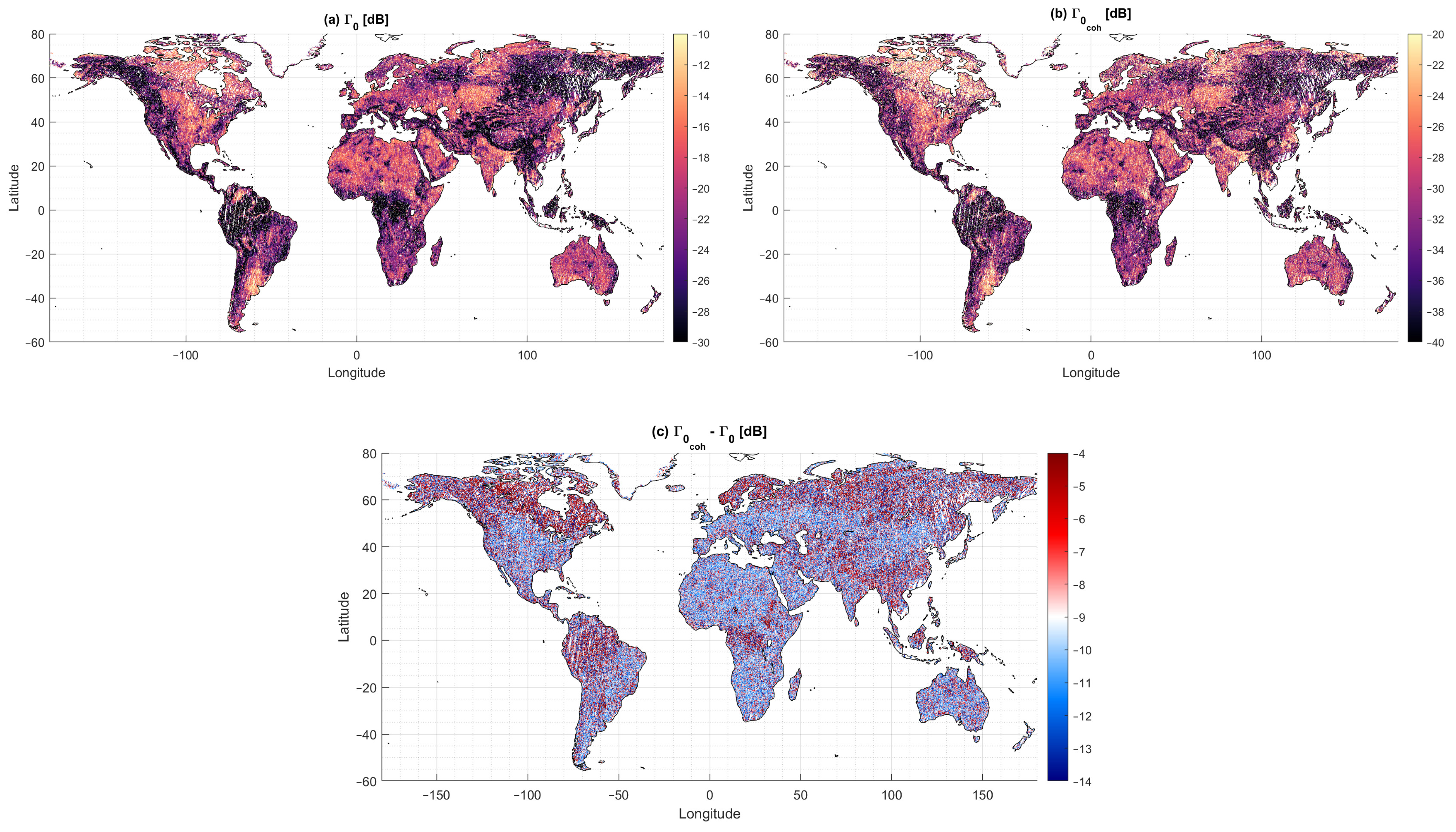
4.1. Coherent Component Reflectivity

The measurements collected by SMAP-R and processed into a coherent component reflectivity, following Equations (10)–(16), are presented in Figure 1, and compared to the total power waveform reflectivity. The total power waveform and the coherent component have the same sensitivity to terrain features but present an average difference of −9.2 dB and an unbiased root mean square difference (ubRMSD) of 3.4 dB. Some specific regions present more noticeable differences between both components. High latitude areas in the winter period, where the soil is mostly covered by snow or ice, present stronger coherent reflections.

Densely vegetated areas such as Boreal forests, or the Congo and the Amazon rainforests present a lower difference between the coherent and the incoherent component, in accordance with simulations from [56], with both components severely affected by the attenuation of the vegetation volume scattering [23]. Other regions present a consistent bias with variations of ±1 dB, but with a consistent bias of ~−9 dB, indicating that the coherent component is an order of magnitude smaller than the total power waveform (~10%), hence indicating that from the total power received in Equation (1) most of it corresponds to the incoherent component, and some of it corresponds to the coherent one. It should be noted that these initial findings suggest that the incoherent component, when integrated over 30 ms, dominates the reflection. Furthermore, as other studies have previously concluded over specific geographical areas [39,57], our initial findings suggest that the GO model would be better suited for modeling the topography effect of GNSS-R over land.

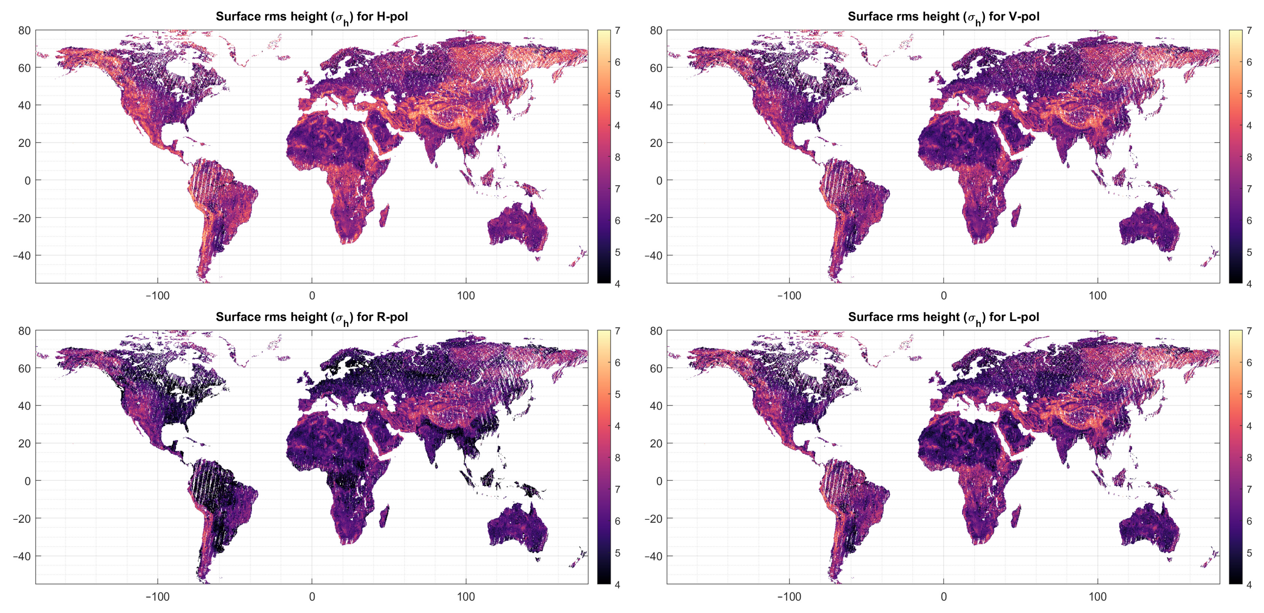
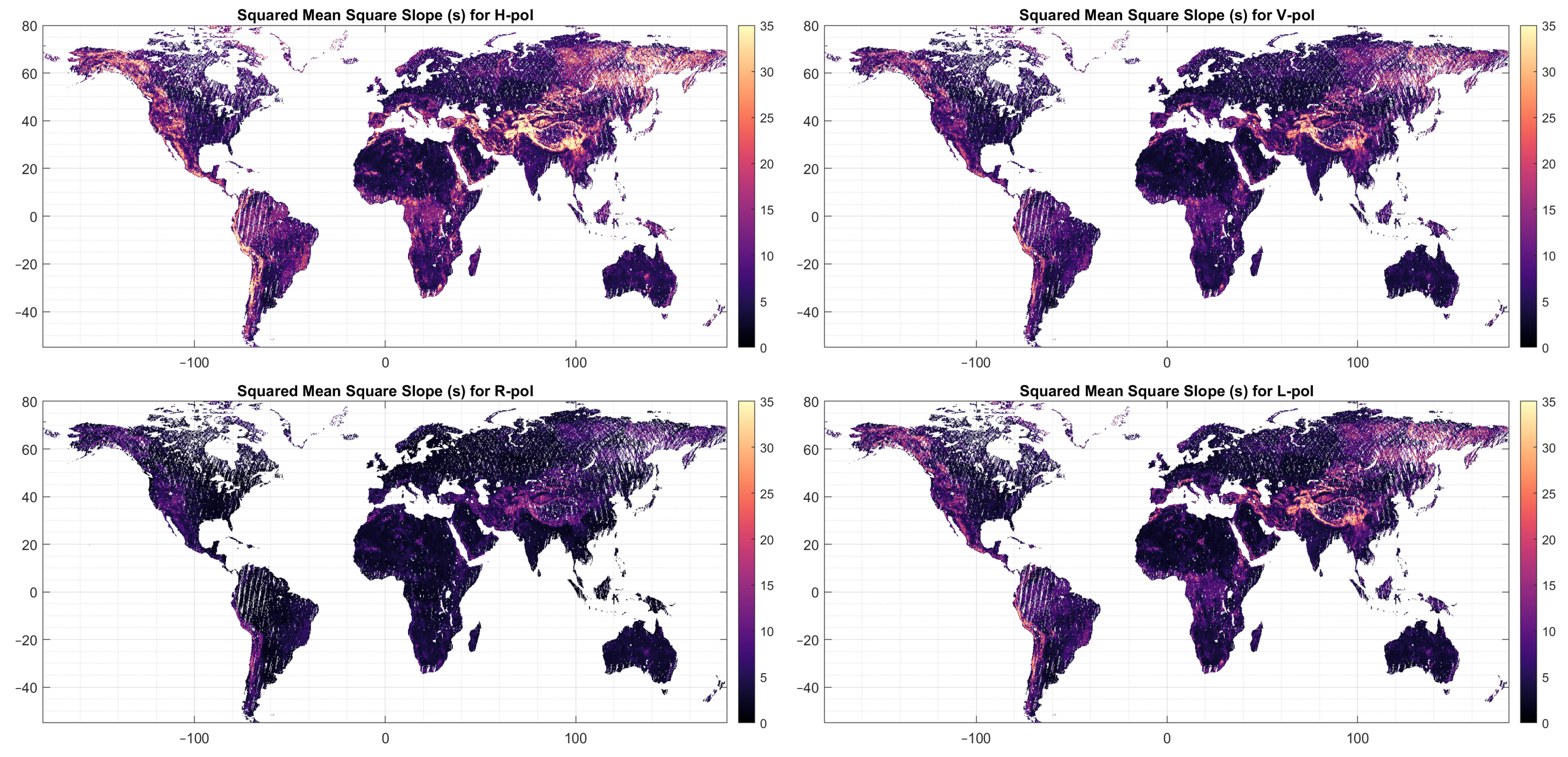
4.2. Multiple Polarization Roughness Estimates

The methodology from Section 3.2 is implemented using the coherent and incoherent components from Figure 1, and its corresponding Stokes parameters. The surface rms height (${\sigma }_h$) is estimated from Equation (24), and the slope rms (s) is estimated from Equation (25). The results are presented in Figure 2 for H, V, R, and L signals, respectively, for ${\sigma }_h$, and in Figure 3 for the slope rms (s).

The surface roughness parameter shows slight differences depending on the polarization selected. ${{\sigma }_h}_H$ (rms height for H-pol) has an average value of 5.66 cm, ${{\sigma }_h}_V$ of 5.40 cm, ${{\sigma }_h}_R$ of 4.94 cm, and ${{\sigma }_h}_L$ of 5.20 cm. The standard deviation of each roughness is ~0.82 cm. Moreover, the ubRMSD and correlation coefficient between the different roughness values are summarized in

Table 2. The ubRMSD between PO modeled rms height (${\sigma }_h$) at different polarizations. Units are in centimeters.

ubRMSD	${{\mathit{\sigma }}_{\mathit{h}}}_{\mathit{H}}$	${{\mathit{\sigma }}_{\mathit{h}}}_{\mathit{V}}$	${{\mathit{\sigma }}_{\mathit{h}}}_{\mathit{R}}$	${{\mathit{\sigma }}_{\mathit{h}}}_{\mathit{L}}$
${{\sigma }_h}_H$
${{\sigma }_h}_V$	0.19
${{\sigma }_h}_R$	0.53	0.59
${{\sigma }_h}_L$	0.14	0.14	0.58

and

Table 3. Pearson Correlation (R) between PO modeled rms height (${\sigma }_h$) at different polarizations.

R	${{\mathit{\sigma }}_{\mathit{h}}}_{\mathit{H}}$	${{\mathit{\sigma }}_{\mathit{h}}}_{\mathit{V}}$	${{\mathit{\sigma }}_{\mathit{h}}}_{\mathit{R}}$	${{\mathit{\sigma }}_{\mathit{h}}}_{\mathit{L}}$
${{\sigma }_h}_H$
${{\sigma }_h}_V$	0.97
${{\sigma }_h}_R$	0.79	0.73
${{\sigma }_h}_L$	0.99	0.99	0.76

. All four ${\sigma }_h$ present slight biases between them, but with a high correlation coefficient between the H, V, and L, with a small ubRMSD. However, this is not the case for the roughness in the RHCP polarization. As seen in the map from Figure 2, very small roughness values are shown in vegetated areas.

Analogously to Table 2 and Table 3,

Table 4. The ubRMSD between GO modeled surface slope rms (s) using different polarizations.

ubRMSD	${\mathit{s}}_{\mathit{H}}$	${\mathit{s}}_{\mathit{V}}$	${\mathit{s}}_{\mathit{R}}$	${\mathit{s}}_{\mathit{L}}$
$s_H$
$s_V$	3.94
$s_R$	6.94	3.97
$s_L$	3.83	0.81	3.56

and

Table 5. Pearson Correlation (R) between GO modeled surface slope rms (s) using different polarizations.

R	${\mathit{s}}_{\mathit{H}}$	${\mathit{s}}_{\mathit{V}}$	${\mathit{s}}_{\mathit{R}}$	${\mathit{s}}_{\mathit{L}}$
$s_H$
$s_V$	0.97
$s_R$	0.86	0.78
$s_L$	0.99	0.99	0.83

present the same coefficients for the slope rms (s).

Looking at the retrieved slope (s) in Figure 3, we see average values of 9.28, 6.75, 4.01, and 5.92 for H, V, R, L, and its standard deviations are 9.52, 5.92, 3.18, 5.75. In this case, it is surprising the very small bias and error between the surface slope at V polarization and L polarization, even larger than in the rms height (${\sigma }_h$) case.

The results show slight differences among the different polarizations. In terms of correlation between the products, PO and GO modeled roughness shows a very high correlation between H, V, and L, but a lower correlation with the R signal. The R signal SNR being lower than H, V, or L, as shown in [53], may bury the RHCP component under the noise, making it impossible to measure and resulting in an increased bias in the retrieved roughness. As for H, V, or L, the ubRMSD is approximately 3% of the actual value, indicating that the assumption of a negligible cross-polarization component only produces a 3% error in the surface roughness retrieval, for the PO model. However, in the GO case, the ubRMSD is higher due to the logarithmic shape of the rms slope (s), with respect to the average value. Still, this ubRMSD is two times lower than the slope rms standard deviation. This finding confirms that the assumption of negligible cross-polarization does not significantly bias the results, but it should be taken into account for very accurate retrievals. Note that, simulation studies on polarimetric roughness have studied the effects of scattering in HR, VR, LR, and RR, showing that the real and imaginary parts of the Fresnel reflection coefficient at h and v polarization are slightly affected by the surface roughness [58].

Additionally, despite ${\sigma }_h$ and s represent different physical phenomena, the correlation between them is noticeable. In this regard, ${\sigma }_h$ and s are related by:

$${\sigma }_h=a\cdot \mathrm{l}\mathrm{n}\left(s\right)+b,$$

(26)

where a and b are two coefficients that can be estimated via least squares.

Table 6. Coefficients and correlation between the model described by Equation (26).

Model	a	b	R	RMSD
$s_H/{\sigma }_{h_H}$	0.86	4.08	0.85	0.42
$s_V/{\sigma }_{h_V}$	0.91	3.97	0.84	0.40
$s_R/{\sigma }_{h_R}$	1.08	3.72	0.87	0.38
$s_L/{\sigma }_{h_R}$	0.94	3.90	0.84	0.43

summarizes the coefficients (a and b), the correlation coefficient, and the root mean square difference (RMSD) of the fit. Note that, the units of ${\sigma }_h$ are centimeters.

The results are highly consistent for the four different parameters, with a high correlation coefficient, and very similar parameters, a, and b, that link both magnitudes. This similarity between both methods is linked to the fact that the roughness effect, simulated via the coherent or incoherent component, is similar. The scattered wave coherently integrated for 30 ms, and modeled via the PO model produces a coefficient that is proportional to the incoherently averaged waveform modeled using the GO model. This implies that the signal at 30 ms coherent integration is neither coherent nor incoherent, but a mix of both since the GO model has a formulation to relate to the PO model at the selected integration time. It is worth noting that the RMSD between the fitted GO and the PO model is approximately 0.4 cm, equivalent to around 8% of the average rms height. This means that the difference between the PO and the GO models leads to an error of approximately 8% in the retrieved rms height.

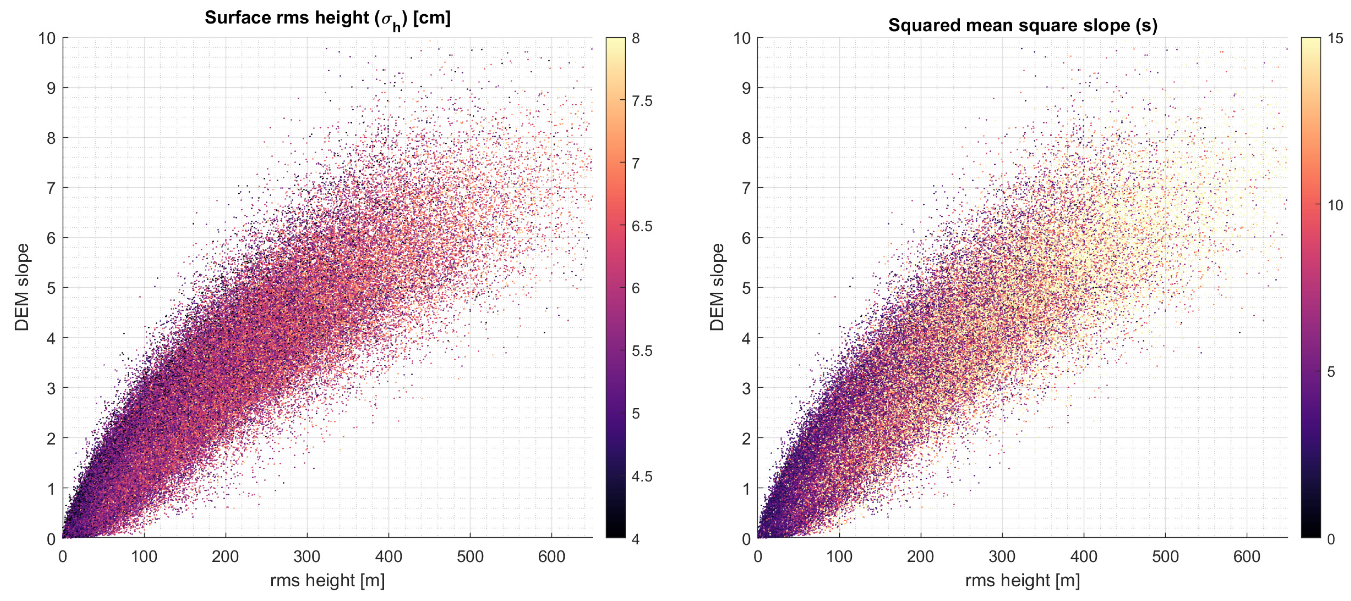
To further analyze the similarity between the rms height and the rms slope, both retrieved magnitudes are compared to the actual DEMSTD and DEMSLPSTD described in Table 1. Note that, DEMSTD is commonly known as the surface height rms, and DEMSLPSTD is the surface slope rms. Given its similarity with other roughness coefficients, we will only compute this for the L polarization. The scatter plot for both ${\sigma }_h$ and s are shown in Figure 4.

In order to relate the DEM rms height (e.g., DEMSTD) to the PO model, we would require a vertical and horizontal resolution of the DEM better than the signal wavelength ([42], p. 423), which is not feasible. However, several studies dealing with different DEM resolutions conclude that a resolution change basically produced a scale on the rms height product [55,59] (e.g., if one wants an equivalent resolution of 1 cm from a 9 km product, the resultant rms height shall be scaled by the ratio of resolutions). In our case, the base resolution of the DEM used here is 30 m, and the standard deviation has been computed and upscaled to larger patches of 9 km.

As can be seen, the slope rms presents a slightly higher sensitivity to the DEM slope (DEMSLPSTD, ${\sigma }_{SLP}$) and rms height (DEMSTD, ${\sigma }_{DEM}$) variations. The correlation coefficient between ${\sigma }_{DEM}$ and ${\sigma }_{SLP}$ and ${\sigma }_h$ are 0.39 and 0.38, while for s are 0.54 and 0.52, respectively. Different models are tested to find a relationship between both magnitudes and ${\sigma }_h$ and s. It is found that the following linear relationship has a large correlation between DEMSTD and DEMSLPSTD and s:

$$s=3.83+0.0386\cdot {\sigma }_{DEM}-0.0757\cdot {\sigma }_{SLP}.$$

(27)

This linear fit presents a correlation coefficient of 0.54, with an RMSD of 4.84. A similar fit can be implemented for the ${\sigma }_h$ parameter, however, the correlation and RMSD are, R = 0.40, and RMSD of 0.80 cm for the equation:

$${\sigma }_h=4.96+0.0036\cdot {\sigma }_{DEM}+0.039\cdot {\sigma }_{SLP}.$$

(28)

Note that, the resolution of our ${\sigma }_{DEM}$ is meters, ranging from 0 to 500 m, with a resolution of 9 km. By scaling the magnitude by 0.0036 the model is telling us that ${\sigma }_h$ scale is ~277 times smaller than the 9 km resolution from the DEMSTD product used, which is ~30 m, 10 times the size of the GNSS chip at L2C.

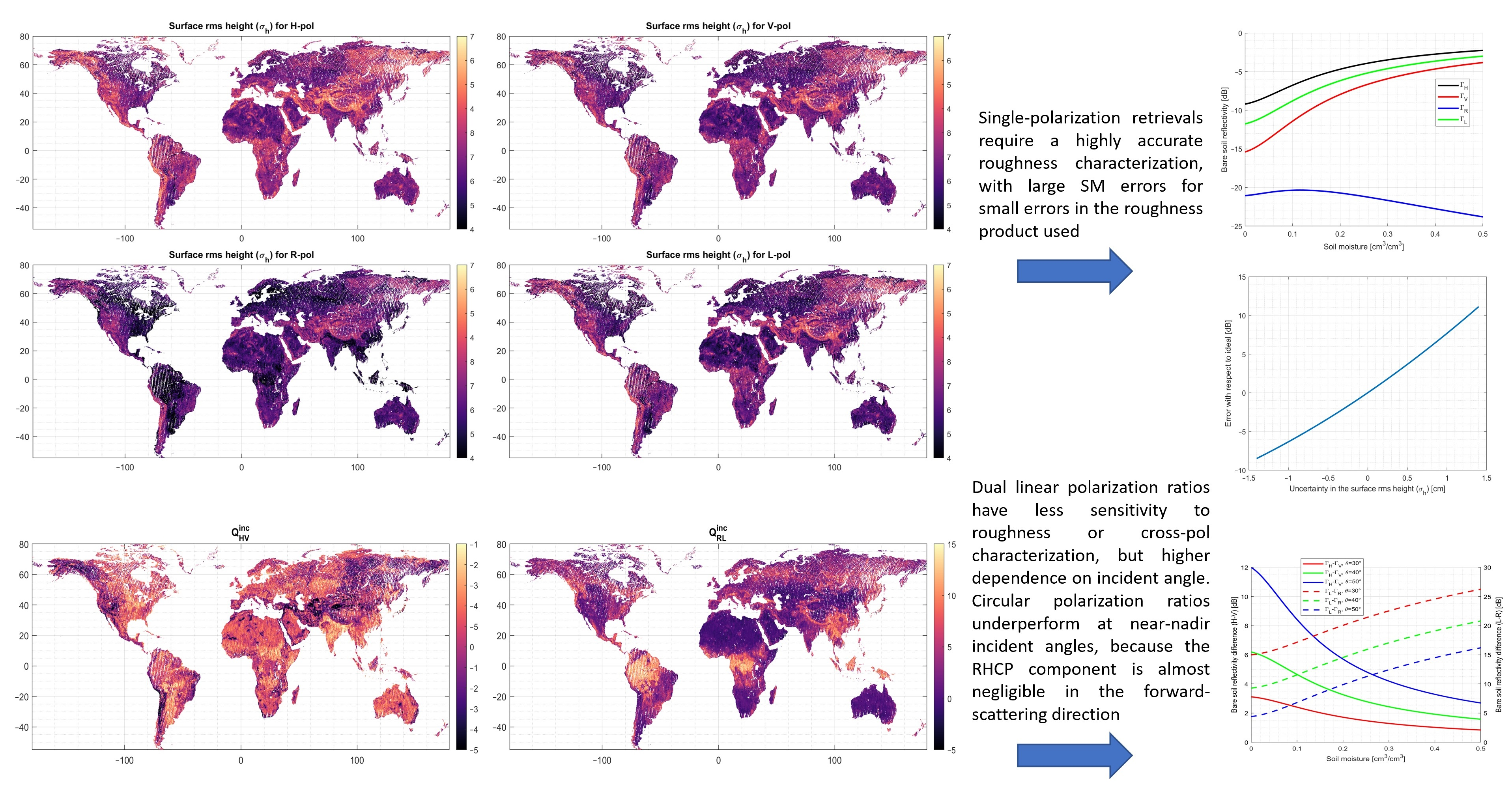
4.3. Roughness Uncertainty on Soil Moisture Retrievals

Both ${\sigma }_h$ and $s$ have been shown to be correlated to DEMSTD and DEMSLPSTD. However, the non-negligible RMSD of this parameter could prevent the implementation of Fresnel reflection coefficient inversion algorithms to estimate surface soil moisture [21].

In this section, we will use the model with ${\sigma }_h$, estimated via Equation (24) with an RMSD of 0.80 cm, to quantify the soil moisture estimation uncertainty. We now introduce the error metric due to the roughness uncertainty as:

$${\epsilon }_{{\sigma }_h}=10{\mathrm{l}\mathrm{o}\mathrm{g}}_{10}\left(e^{-4k^2{\sigma }_h^{2}co{s}^2\left(\theta \right)}\right)-10{\mathrm{l}\mathrm{o}\mathrm{g}}_{10}\left(e^{-4k^2{\left({\sigma }_h+\epsilon \right)}^{2}co{s}^2\left(\theta \right)}\right),$$

(29)

where ε is the error estimating the surface rms height parameter.

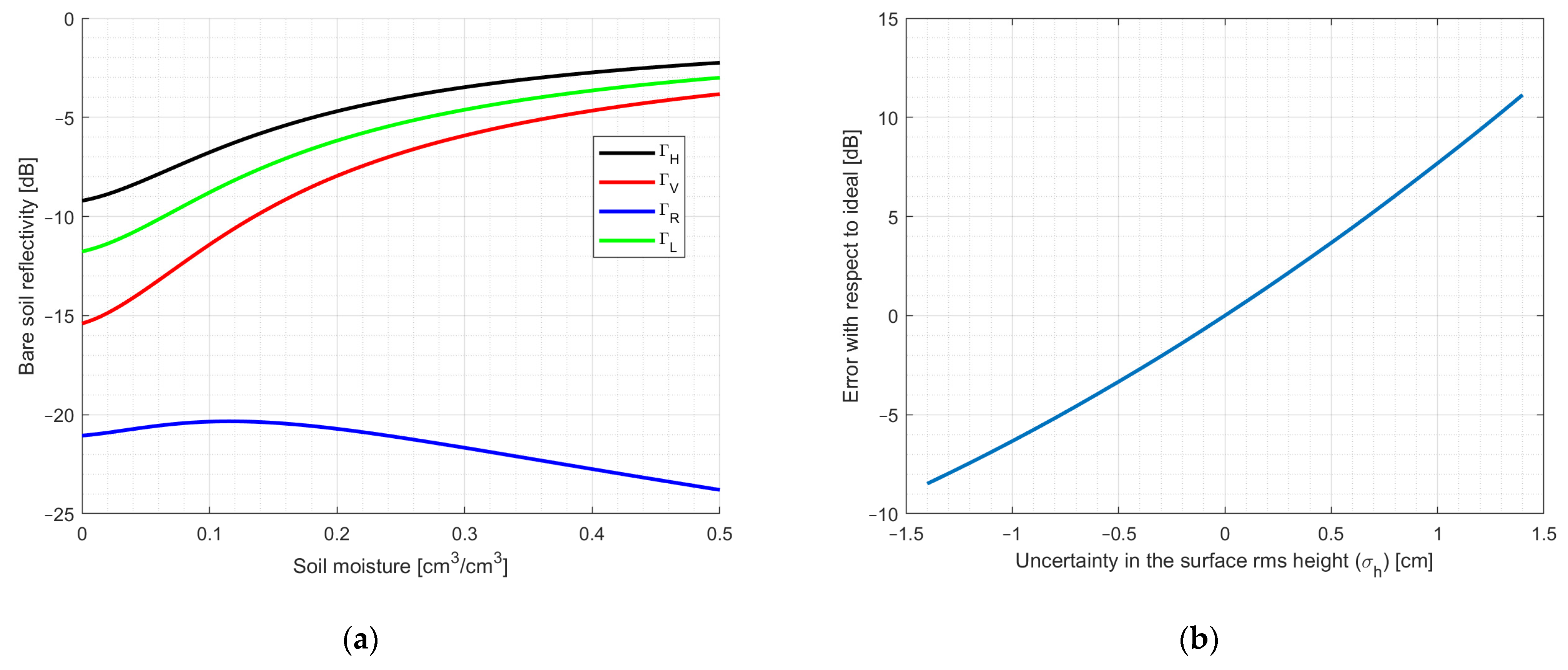
The impact of different values of ε is shown in Figure 5 assuming an average value of ${\sigma }_h$ = 5.2 cm, its average value for L-polarization, and $\theta =40°.$

A surface roughness uncertainty of 0.8 cm (the standard deviation of the fit from Equation (28)) produces an error of ${\epsilon }_{{\sigma }_h}=$ 5.0 dB, producing an error in the soil moisture retrieval of ~0.12 cm³/cm³ for ${\Gamma }_V$, and even larger for other polarimetric components as the ${\Gamma }_H$ or ${\Gamma }_L$, with errors higher than 0.2 cm³/cm³ for the LHCP component. These large differences in single-polarization approaches suggest that by only using single-polarization measurements, soil moisture retrievals might not be feasible for single-pass retrievals if the surface roughness is not accurately modeled. In other words, because the correlation coefficient is very low with respect to the actual GNSS-R reflectivity measurements, retrievals using the Tau-Omega model, using VOD, and estimating surface roughness from DEM models, will not produce an accurate soil moisture product. As indicated in ([42], p. 423) an acceptable DEM base product to produce the small-scale surface roughness that is required in the coherent model needs to be comparable to $\lambda$, which is not feasible nowadays for a global coverage approach.

4.4. Dual-Polarization Differential Roughness Estimates

Solving the roughness effect for a single polarization gives us the possibility for single-polarization soil moisture retrievals using any polarization combination. However, the algorithm is highly dependent on the accuracy of the roughness map. To overcome this issue, combined polarimetric retrievals can be used to mitigate the effect of roughness. This approach has been proposed by several pieces of research [28,42,60,61] to allow a higher quality soil moisture estimation without the need to accurately model the surface roughness, reducing the error. As in the single-polarization case, we define an error term by comparing the measured reflectivity ratio with the Fresnel reflection coefficient ratio:

$$Q_{pq}\left[dB\right]=10{\log }_{10}\frac{{\Gamma }_p}{{\Gamma }_q}-10{\log }_{10}\frac{{\left|R_p\left(\theta \right)\right|}^2}{{\left|R_q\left(\theta \right)\right|}^2},$$

(30)

Being p and q two orthogonal polarizations, and Q polarization coupling factor [28]. Note that, VOD and roughness parameters are neglected here, and both are simplified by the Q parameter.

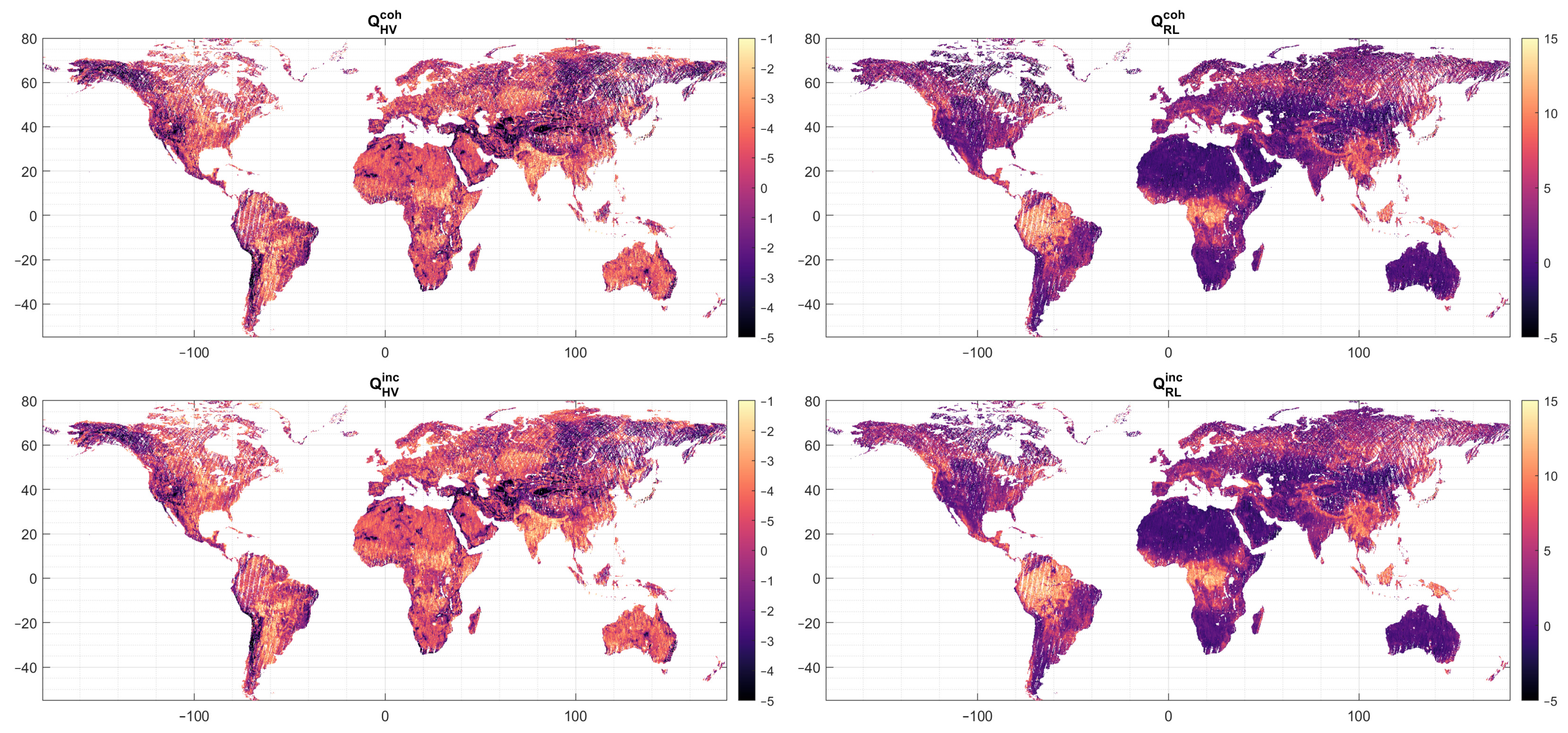
Results for $Q_{pq}$ for p = {H,R} and q = {V,L} for both ${\Gamma }^{coh}$ and ${\Gamma }^{inc}$ are shown in Figure 6. As can be seen, results are very similar for the coherent and incoherent cases. For the HV case, the correlation between the coherent and the incoherent is 0.88, with an RMSD of 0.61 dB. The average Q_HV value is −2.2 dB, and the standard deviation is 1.3 dB. First, these results indicate that the SMAP-R captured H/V ratio presents a ~2.29 dB bias with respect to the theoretical one. The analysis of this bias was discussed in [52] to be produced by the GPS L2 antenna axial ratio for blocks IIR or newer [62,63].

For Q_RL the average value is 2.72 dB with a standard deviation of 3.86 dB, and the correlation between the coherent and incoherent cases is 0.87 and 1.33 dB, respectively.

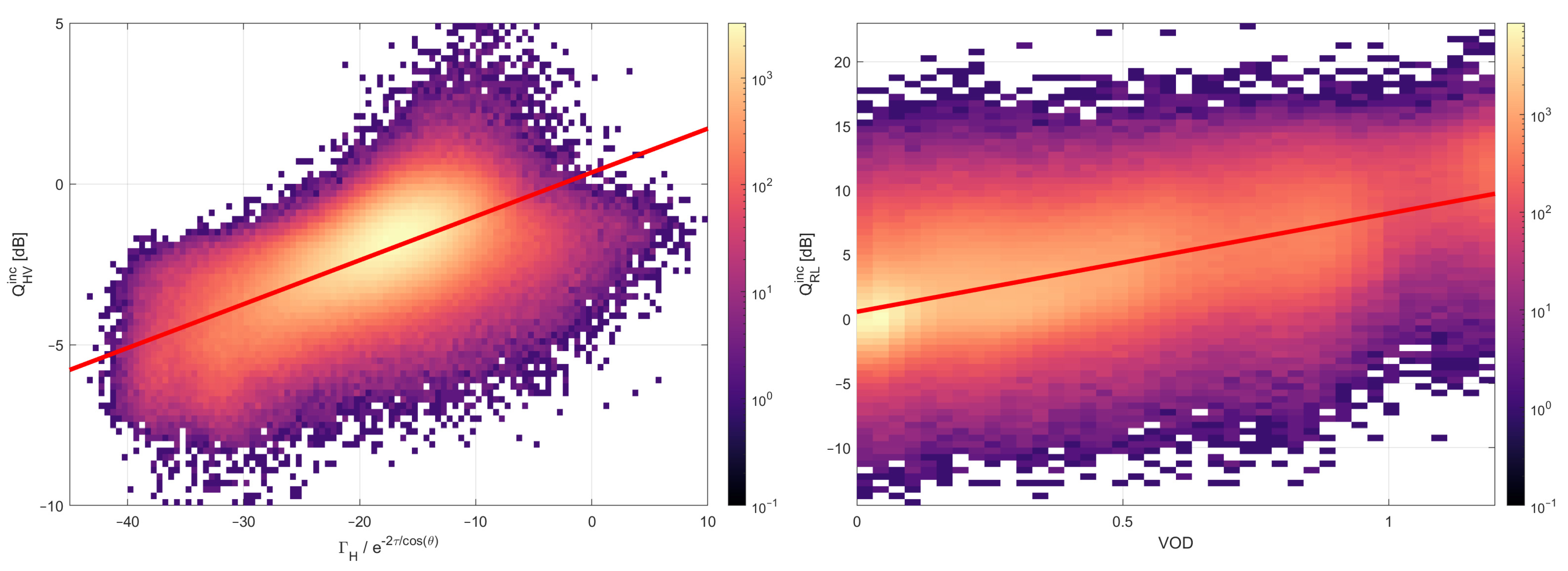
In this case, the Q_HV seems uncorrelated with any surface parameter (e.g., DEM), but it does correlate with some parameters of the reflection, as the incoherent reflectivity from Equations (5)–(7), once calibrated by VOD:

$$Q_{HV}^{inc}\left[dB\right]=0.1364\cdot 10{\log }_{10}\left(\frac{{\stackrel{-}{\mathsf{\Gamma }}}_H^{inc}}{e^{\frac{-2\tau }{\cos \left(\theta \right)}}}\right)+0.35,$$

(31)

With an RMSD of 0.97 dB and a correlation coefficient of 0.64. If VOD is not compensated, the correlation coefficient is lowered down to 0.55 and the RMSD increases up to 1.09 dB. Results for the coherent part show a lower correlation coefficient (0.4) and larger RMSD (1.38), which could indicate that this parameter is more sensitive to incoherent scattering rather than specular scattering.

On the contrary, Q_RL is correlated with vegetation, notably in areas with large vegetation, e.g., Congo or Amazonian rainforests. VOD and Q_RL are related via the linear relationship:

$$Q_{RL}^{inc}\left[dB\right]=7.7612\cdot \tau +0.48.$$

(32)

In this case, the correlation is 0.65, and the RMSD is 2.93 dB. The scatter-density plots of both fits are shown in Figure 7.

4.5. Dual-Polarization Roughness Uncertainty Impact on Soil Moisture Retrievals

Analogously to Section 4.3, the same analysis is conducted here for dual-polarization SM retrievals. Equation (30) either for $Q_{HV}$ or $Q_{LR}$ already gives the amount of dB between the modeled value from SMAP SM and the measured polarimetric ratio.

The impact of a bad estimation of the Q parameter on soil moisture retrievals is presented in Figure 8.

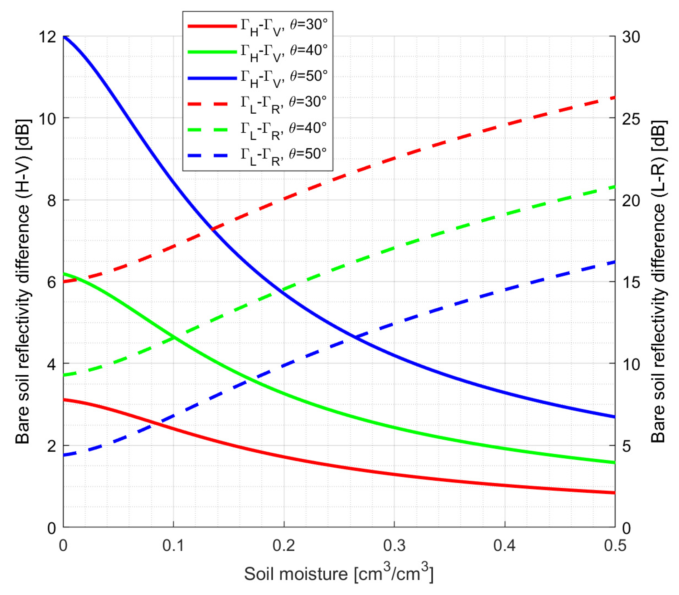
In this case, an uncertainty or error of ±2 dB (e.g., two times the uncertainty of $Q_{HV}$), for an incidence angle of ~30°, will produce a soil moisture error of ~0.3 cm³/cm³, but for incidence angles larger than 30° (e.g., 40° or 50°), the 1-sigma error would be ~0.05 cm³/cm³, and the 2-sigma error ~0.08 cm³/cm³. For the circular polarization case, a 2-dB error represents, for any of the presented incidence angle combinations, a soil moisture 1-sigma error lower than 0.05 cm³/cm³ and a 2-sigma error lower than 0.08 cm³/cm³. However, the RHCP component cannot be always received at any arbitrary incidence angle due to its very low reflectivity.

5. Discussion

5.1. Land Reflection: Coherent vs. Incoherent Approach

In this study, the coherent and incoherent components of the GNSS-R waveform have been separated and either the rms height for the PO model and surface slope and for the GO model, have been retrieved. This is feasible thanks to the SMAP high antenna gain, which allows the detection of the GNSS reflection even without incoherent integration. However, coherent component retrieval is not trivial for other systems that require longer incoherent integrations, and the signal coherency cannot be preserved due to terrain fluctuations. In such cases, incoherent components should be used to estimate the roughness. As it has been presented in Section 4.1, the coherent component and the total power waveform present a ~−9 dB consistent bias and an ubRMSD of 3.4 dB. Computing the roughness with coherent or incoherent components might impact a bias in the retrieved magnitude. Results in Section 4.2 shows that the roughness coefficient retrieved using the coherent at 30 ms integration, and the incoherent component can be easily related using a logarithmic model. This indicates that neither the reflected waveform is coherent nor incoherent, but as modeled in Equation (1), a combination of both, but being the incoherent component dominant.

The PO model bases the roughness effect on the rms height of the surface, while the GO model is a high-frequency approximation for the PO model when the surface is rough enough with respect to the signal wavelength. In this regard, limits were defined in the Kirchhoff scattering model to define the regimes of the PO and GO models. In some of the literature, the limit for the PO model is defined for $\frac{2\pi }{\lambda }{\sigma }_h<3$, while for the GO model, the limit is defined for $\frac{2\pi }{\lambda }{\sigma }_h\ge 3$ ([42], p. 428). Our findings on ${\sigma }_h$ point out a roughness comprised between 4 and 8 cm. For GPS L2C band, $\frac{2\pi }{\lambda }{\sigma }_h=[1.07,2.14]$, for ${\sigma }_h=\left[4,8\right]$ cm, and for GPS L1, the values are $\frac{2\pi }{\lambda }{\sigma }_h=[1.32,2.64]$. However, other studies have validated using experimental data that the limit for PO and GO approximations differ from the originally proposed value [64], being PO limited by $\frac{2\pi }{\lambda }{\sigma }_h<0.75$ and GO limited by $\frac{2\pi }{\lambda }{\sigma }_h>1.75$. In this second case, and given the range of ${\sigma }_h$ found in this study, and supported by other studies [39,57], it seems that GNSS reflections can be better approximated by a high—frequency approximation of the PO model (i.e., the GO model) rather than by the classical PO model, as also confirmed by the results in Section 4.2. This can be also explained by the higher power received in the total power waveform compared to the coherent component part, and the larger correlation of the GO model with the SMAP DEMSLPSTD product. Hence, both results seem to indicate that, in general, the specular forward-scattering over land at GPS bands could be better modeled by the GO approximation due to large-scale roughness variations, rather than small roughness effects modeled using the PO approximation. Note that advanced models such as the Analytical Kirchhoff Solution (AKS), have shown promising results in modeling the impact of roughness on GNSS-R signals [57]. However, these models lack a closed analytical solution that can isolate the roughness parameter to study its relationship with physical quantities for global retrievals.

5.2. Antenna Requirements for Soil Moisture Retrievals Using Polarimetric GNSS-R

To summarize the findings in Section 4.4, combined RHCP-LHCP measurements provide better performance for soil moisture retrievals. Moreover, the use of VOD as a proxy to estimate $Q_{LR}$ provides the combination of RHCP and LHCP signals with the best soil moisture estimation, where only H-V antennas can provide similar errors at $\theta$ = 40°. However, as it is discussed in [51,53], the reflectivity at RHCP at incidences angles lower than 55° is 15–25 dB lower than the LHCP reflectivity. At $\theta$ = 40°, this difference is ~10 dB for dry soils, and more than 15 dB for 0.2 cm³/cm³ or higher SM, masking the RHCP signal below the receivers’ noise floor. In such cases, the H/V component shows similar performances as the L/R component for soil moisture retrieval.

As shown in Figure 8, at lower angles (30° and smaller), the RHCP signal suffers attenuations up to 25 dB larger than the LHCP signals for high soil moisture values. For current antenna configurations of four or six patches (e.g., CYGNSS [65] or FSSCat [9], providing ~12 dB gain and ~40° half-power beam-width), such large attenuations may cause the GNSS-R signal to be well below the receiver’s noise floor. As an example, current LHCP observations over land show SNRs between 0 and 15 dB (avg. ~5 dB and std. ~5 dB [66]).

At higher angles (50° and higher), where both RHCP and LHCP are on the same range, the vegetation attenuation due to the high incidence angle (e.g., Equation (1)) can be large enough to destroy both L and R components of the signal.

Hence, following the model presented in Figure 8, not many reflections collected by an RHCP antenna would be above the receiver’s noise floor. One way to mitigate this issue is by using H and V polarized antennas, with higher SNRs than the RHCP, and computing the Stokes parameters of the received signal as shown in this manuscript and further detailed in [18]. The estimated synthetic LHCP/RHCP ratio would be as good as the S₀ SNR, meaning that no RHCP component could be retrieved if the total H and V SNR are too low. Even though, one could still perform polarimetric retrievals using H and V components even at low SNRs, and use the four polarization (H/V and synthetic L/R) when the S₀ SNR is high enough.

6. Conclusions

This manuscript has presented different methodologies to estimate the effect of the surface roughness in polarimetric GNSS-R. Data from SMAP-R has been collocated to SMAP L3 enhanced dataset. Soil moisture, VOD, and static SMAP ancillary files such as DEMSTD or DEMSLPSTD, products derived from the DEM, have been used. A methodology to estimate the surface rms height using the coherent component, and the surface slope rms using the incoherent component have been presented and evaluated. First, a single-polarization approach has been implemented for all four possible polarizations, H, V, R, and L, and for coherent and incoherent components. The roughness product assuming coherent reflection has shown a large correlation with the roughness product estimated using incoherent reflection. The correlation between these roughness products and SMAP static DEM products have been evaluated.

Potential soil moisture errors are analyzed for a given ${\sigma }_h$ uncertainty of its half standard deviation. This shows errors on the order of 0.12 cm³/cm³ for the V-polarization case, which presents its maximum polarimetric sensitivity at 40° of incidence angle.

Additionally, a dual-polarization model has been presented using the ratio (or difference in dB) between either L-R and H-V components, named polarization decoupling. Results for the linear polarizations show that even with an uncertainty of 2-sigma when estimating the polarization decoupling for $HV$ polarization. A linear model based on the SMAP-R surface reflectivity and SMAP VOD product is shown to be linearly dependent to the $Q_{HV}$ parameter. Following this approach, a soil moisture product can be estimated with 2-sigma errors of ~0.08 cm³/cm³ for incidence angles close to 40°. For the circular polarization case, it is found that the $Q_{LR}$ parameter linearly correlates with $\mathrm{V}\mathrm{O}\mathrm{D}$, and this can be used with a linear regression to estimate the polarization difference. In this case, if the RHCP component is strong enough, a soil moisture product with a 2-sigma error of ~ 0.08 cm³/cm³ can be produced at virtually any incidence angle.

Dual-polarization retrievals, where the ratio between H and V or L and R are used, allow for soil moisture retrieval without the need for absolute signal calibration. Hence, providing a more robust and independent soil moisture retrieval algorithm.

Finally, the importance of choosing the proper antenna polarization configuration soil moisture retrieval using polarimetric GNSS-R signals is discussed, showing that synthetic RHCP/LHCP component can be retrieved by means of slightly higher directive H/V antennas and using the Stokes parameter (as performed in this manuscript), and on such cases that the RHCP is masked under the receiver’s noise floor, differential H/V algorithms could be used to retrieve soil moisture.

References

- Ruf, C.; Unwin, M.; Dickinson, J.; Rose, R.; Rose, D.; Vincent, M.; Lyons, A. CYGNSS: Enabling the Future of Hurricane Prediction [Remote Sensing Satellites]. IEEE Geosci. Remote Sens. Mag. 2013, 1, 52–67. [Google Scholar] [CrossRef]
- Chew, C.; Reager, J.T.; Small, E. CYGNSS data map flood inundation during the 2017 Atlantic hurricane season. Sci. Rep. 2018, 8, 9336. [Google Scholar] [CrossRef]
- Clarizia, M.P.; Pierdicca, N.; Costantini, F.; Floury, N. Analysis of CYGNSS Data for Soil Moisture Retrieval. IEEE J. Sel. Top. Appl. Earth Obs. Remote Sens. 2019, 12, 2227–2235. [Google Scholar] [CrossRef]
- Wan, W.; Liu, B.; Guo, Z.; Lu, F.; Niu, X.; Li, H.; Ji, R.; Cheng, J.; Li, W.; Chen, X.; et al. Initial Evaluation of the First Chinese GNSS-R Mission BuFeng-1 A/B for Soil Moisture Estimation. IEEE Geosci. Remote Sens. Lett. 2021, 19, 1–5. [Google Scholar] [CrossRef]
- Jing, C.; Niu, X.; Duan, C.; Lu, F.; Di, G.; Yang, X. Sea Surface Wind Speed Retrieval from the First Chinese GNSS-R Mission: Technique and Preliminary Results. Remote Sens. 2019, 11, 3013. [Google Scholar] [CrossRef] [Green Version]
- Camps, A.; Munoz-Martin, J.; Ruiz-De-Azua, J.; Fernandez, L.; Perez-Portero, A.; Llaveria, D.; Herbert, C.; Pablos, M.; Golkar, A.; Gutierrrez, A.; et al. FSSCat Mission Description and First Scientific Results of the FMPL-2 Onboard 3CAT-5/A. In Proceedings of the 2021 IEEE International Geoscience and Remote Sensing Symposium IGARSS, Brussels, Belgium, 11–16 July 2021; pp. 1291–1294. [Google Scholar] [CrossRef]
- Munoz-Martin, J.; Llaveria, D.; Herbert, C.; Pablos, M.; Park, H.; Camps, A. Soil Moisture Estimation Synergy Using GNSS-R and L-Band Microwave Radiometry Data from FSSCat/FMPL-2. Remote Sens. 2021, 13, 994. [Google Scholar] [CrossRef]
- Munoz-Martin, J.F.; Camps, A. Sea Surface Salinity and Wind Speed Retrievals Using GNSS-R and L-Band Microwave Radiometry Data from FMPL-2 Onboard the FSSCat Mission. Remote Sens. 2021, 13, 3224. [Google Scholar] [CrossRef]
- Munoz-Martin, J.F.; Capon, L.F.; Ruiz-De-Azua, J.A.; Camps, A. The Flexible Microwave Payload-2: A SDR-Based GNSS-Reflectometer and L-Band Radiometer for CubeSats. IEEE J. Sel. Top. Appl. Earth Obs. Remote Sens. 2020, 13, 1298–1311. [Google Scholar] [CrossRef]
- Jales, P.; Esterhuizen, S.; Masters, D.; Nguyen, V.; Nogués-Correig, O.; Yuasa, T.; Cartwright, J. The new Spire GNSS-R satellite missions and products. Image Signal Process. Remote Sens. XXVI 2020, 11533, 1153316. [Google Scholar] [CrossRef]
- Han, Y.; Luo, J.; Xu, X. On the Constellation Design of Multi-GNSS Reflectometry Mission Using the Particle Swarm Optimization Algorithm. Atmosphere 2019, 10, 807. [Google Scholar] [CrossRef] [Green Version]
- Xu, X.; Ju, Z.; Luo, J. Design of Constellations for GNSS Reflectometry Mission Using the Multiobjective Evolutionary Algorithms. IEEE Trans. Geosci. Remote Sens. 2022, 60, 1–15. [Google Scholar] [CrossRef]
- Entekhabi, D.; Yueh, S.; O’neill, P.; Kellogg, K.; Allen, A.; Bindlish, R.; Brown, M.E.; Chan, S.; Colliander, A.; Crow, W.; et al. SMAP Handbook–Soil Moisture Active Passive: Mapping Soil Moisture and Freeze/Thaw from Space; National Aeronautics and Space Administration, Jet Propulsion Laboratory/California Institute of Technology: Washington, DC, USA, 2014. [Google Scholar]
- Carreno-Luengo, H.; Lowe, S.; Zuffada, C.; Esterhuizen, S.; Oveisgharan, S. Spaceborne GNSS-R from the SMAP Mission: First Assessment of Polarimetric Scatterometry over Land and Cryosphere. Remote Sens. 2017, 9, 362. [Google Scholar] [CrossRef] [Green Version]
- Chew, C.; Lowe, S.; Parazoo, N.; Esterhuizen, S.; Oveisgharan, S.; Podest, E.; Zuffada, C.; Freedman, A. SMAP radar receiver measures land surface freeze/thaw state through capture of forward-scattered L-band signals. Remote Sens. Environ. 2017, 198, 333–344. [Google Scholar] [CrossRef]
- Rodriguez-Alvarez, N.; Misra, S.; Morris, M. The Polarimetric Sensitivity of SMAP-Reflectometry Signals to Crop Growth in the U.S. Corn Belt. Remote Sens. 2020, 12, 1007. [Google Scholar] [CrossRef] [Green Version]
- Rodriguez-Alvarez, N.; Misra, S.; Podest, E.; Morris, M.; Bosch-Lluis, X. The Use of SMAP-Reflectometry in Science Applications: Calibration and Capabilities. Remote Sens. 2019, 11, 2442. [Google Scholar] [CrossRef] [Green Version]
- Munoz-Martin, J.F.; Rodriguez-Alvarez, N.; Bosch-Lluis, X.; Oudrhiri, K. Stokes Parameters Retrieval and Calibration of Hybrid Compact Polarimetric GNSS-R Signals. IEEE Trans. Geosci. Remote Sens. 2022, 60, 1–11. [Google Scholar] [CrossRef]
- GCOS. What Are Essential Climate Variables? Available online: https://gcos.wmo.int/en/essential-climate-variables/about (accessed on 1 October 2022).
- Chew, C.C.; Small, E.E. Soil Moisture Sensing Using Spaceborne GNSS Reflections: Comparison of CYGNSS Reflectivity to SMAP Soil Moisture. Geophys. Res. Lett. 2018, 45, 4049–4057. [Google Scholar] [CrossRef] [Green Version]
- Calabia, A.; Molina, I.; Jin, S. Soil Moisture Content from GNSS Reflectometry Using Dielectric Permittivity from Fresnel Reflection Coefficients. Remote Sens. 2020, 12, 122. [Google Scholar] [CrossRef] [Green Version]
- Yan, Q.; Huang, W.; Jin, S.; Jia, Y. Pan-tropical soil moisture mapping based on a three-layer model from CYGNSS GNSS-R data. Remote Sens. Environ. 2020, 247, 111944. [Google Scholar] [CrossRef]
- Munoz-Martin, J.F.; Pascual, D.; Onrubia, R.; Park, H.; Camps, A.; Rudiger, C.; Walker, J.P.; Monerris, A. Vegetation Canopy Height Retrieval Using L1 and L5 Airborne GNSS-R. IEEE Geosci. Remote Sens. Lett. 2022, 19, 1–5. [Google Scholar] [CrossRef]
- Zribi, M.; Guyon, D.; Motte, E.; Dayau, S.; Wigneron, J.P.; Baghdadi, N.; Pierdicca, N. Performance of GNSS-R GLORI data for biomass estimation over the Landes forest. Int. J. Appl. Earth Obs. Geoinformation 2019, 74, 150–158. [Google Scholar] [CrossRef]
- Gamba, M.T.; Marucco, G.; Pini, M.; Ugazio, S.; Falletti, E.; Presti, L.L. Prototyping a GNSS-Based Passive Radar for UAVs: An Instrument to Classify the Water Content Feature of Lands. Sensors 2015, 15, 28287–28313. [Google Scholar] [CrossRef] [Green Version]
- Rodriguez-Alvarez, N.; Podest, E.; Jensen, K.; McDonald, K.C. Classifying Inundation in a Tropical Wetlands Complex with GNSS-R. Remote Sens. 2019, 11, 1053. [Google Scholar] [CrossRef] [Green Version]
- Wang, J.R.; Engman, E.T.; Mo, T.; Schmugge, T.J.; Shiue, J.C. The Effects of Soil Moisture, Surface Roughness, and Vegetation on L-Band Emission and Backscatter. IEEE Trans. Geosci. Remote Sens. 1987, GE-25, 825–833. [Google Scholar] [CrossRef]
- Chaubell, M.J.; Yueh, S.H.; Dunbar, R.S.; Colliander, A.; Chen, F.; Chan, S.K.; Entekhabi, D.; Bindlish, R.; O’Neill, P.E.; Asanuma, J.; et al. Improved SMAP Dual-Channel Algorithm for the Retrieval of Soil Moisture. IEEE Trans. Geosci. Remote Sens. 2020, 58, 3894–3905. [Google Scholar] [CrossRef]
- Chaubell, J.; Yueh, S.; Entekhabi, D.; Dunbar, S.; Colliander, A.; Xu, X.; Mousavi, M. Analysis of the SMAP Roughness Parameter and the SMAP Vegetation Optical Depth. In Proceedings of the IGARSS 2022–2022 IEEE International Geoscience and Remote Sensing Symposium, Kuala Lumpur, Malaysia, 17–22 July 2022; pp. 4232–4235. [Google Scholar] [CrossRef]
- Park, H.; Camps, A.; Castellvi, J.; Muro, J. Generic Performance Simulator of Spaceborne GNSS-Reflectometer for Land Applications. IEEE J. Sel. Top. Appl. Earth Obs. Remote Sens. 2020, 13, 3179–3191. [Google Scholar] [CrossRef]
- Choudhury, B.J.; Schmugge, T.J.; Chang, A.; Newton, R.W. Effect of surface roughness on the microwave emission from soils. J. Geophys. Res. 1979, 84, 5699–5706. [Google Scholar] [CrossRef]
- Camps, A.; Park, H.; Castellví, J.; Corbera, J.; Ascaso, E. Single-Pass Soil Moisture Retrievals Using GNSS-R: Lessons Learned. Remote Sens. 2020, 12, 2064. [Google Scholar] [CrossRef]
- Yueh, S.H.; Shah, R.; Chaubell, M.J.; Hayashi, A.; Xu, X.; Colliander, A. A Semiempirical Modeling of Soil Moisture, Vegetation, and Surface Roughness Impact on CYGNSS Reflectometry Data. IEEE Trans. Geosci. Remote Sens. 2022, 60, 1–17. [Google Scholar] [CrossRef]
- Camps, A. Spatial Resolution in GNSS-R Under Coherent Scattering. IEEE Geosci. Remote Sens. Lett. 2020, 17, 32–36. [Google Scholar] [CrossRef] [Green Version]
- Johnson, J.T.; Warnick, K.F.; Xu, P. On the Geometrical Optics (Hagfors’ Law) and Physical Optics Approximations for Scattering From Exponentially Correlated Surfaces. IEEE Trans. Geosci. Remote Sens. 2007, 45, 2619–2629. [Google Scholar] [CrossRef]
- Wigneron, J.P.; Chanzy, A.; Kerr, Y.H.; Lawrence, H.; Shi, J.; Escorihuela, M.J.; Mironov, V.; Mialon, A.; Demontoux, F.; de Rosnay, P.; et al. Evaluating an Improved Parameterization of the Soil Emission in L-MEB. IEEE Trans. Geosci. Remote Sens. 2011, 49, 1177–1189. [Google Scholar] [CrossRef]
- Zavorotny, V.U.; Larson, K.M.; Braun, J.J.; Small, E.E.; Gutmann, E.D.; Bilich, A. A Physical Model for GPS Multipath Caused by Land Reflections: Toward Bare Soil Moisture Retrievals. IEEE J. Sel. Top. Appl. Earth Obs. Remote Sens. 2010, 3, 100–110. [Google Scholar] [CrossRef]
- Tronquo, E.; Lievens, H.; Bouchat, J.; Defourny, P.; Baghdadi, N.; Verhoest, N.E.C. Soil Moisture Retrieval Using Multistatic L-Band SAR and Effective Roughness Modeling. Remote Sens. 2022, 14, 1650. [Google Scholar] [CrossRef]
- Ren, B.; Zhu, J.; Tsang, L.; Xu, H. Analytical Kirchhoff Solutions (Aks) and Numerical Kirchhoff Approach (Nka) for First-Principle Calculations of Coherent Waves and Incoherent Waves at p Band and l Band in Signals of Opportunity (Soop). Prog. Electromagn. Res. 2021, 171, 35–73. [Google Scholar] [CrossRef]
- Campbell, J.D.; Akbar, R.; Bringer, A.; Comite, D.; Dente, L.; Gleason, S.T.; Guerriero, L.; Hodges, E.; Johnson, J.T.; Kim, S.-B.; et al. Intercomparison of Electromagnetic Scattering Models for Delay-Doppler Maps Along a CYGNSS Land Track With Topography. IEEE Trans. Geosci. Remote Sens. 2022, 60, 1–13. [Google Scholar] [CrossRef]
- De Roo, R.; Ulaby, F. Bistatic specular scattering from rough dielectric surfaces. IEEE Trans. Antennas Propag. 1994, 42, 220–231. [Google Scholar] [CrossRef]
- Ulaby, F.T.; Long, D.G.; Blackwell, W.J.; Elachi, C.; Fung, A.K.; Ruf, C.; Sarabandi, K.; Zebker, H.A.; Van Zyl, J. Microwave Radar and Radiometric Remote Sensing; The University of Michigan Press: Ann Arbor, MI, USA, 2014; ISBN 0472119354. [Google Scholar]
- Stilla, D.; Zribi, M.; Pierdicca, N.; Baghdadi, N.; Huc, M. Desert Roughness Retrieval Using CYGNSS GNSS-R Data. Remote Sens. 2020, 12, 743. [Google Scholar] [CrossRef] [Green Version]
- Hallikainen, M.T.; Ulaby, F.T.; Dobson, M.C.; El-Rayes, M.A.; Wu, L.-K. Microwave Dielectric Behavior of Wet Soil-Part 1: Empirical Models and Experimental Observations. IEEE Trans. Geosci. Remote Sens. 1985, GE-23, 25–34. [Google Scholar] [CrossRef]
- Munoz-Martin, J.F.; Onrubia, R.; Pascual, D.; Park, H.; Camps, A.; Rüdiger, C.; Walker, J.; Monerris, A. Untangling the Incoherent and Coherent Scattering Components in GNSS-R and Novel Applications. Remote Sens. 2020, 12, 1208. [Google Scholar] [CrossRef] [Green Version]
- Zavorotny, V.; Voronovich, A. Scattering of GPS signals from the ocean with wind remote sensing application. IEEE Trans. Geosci. Remote Sens. 2000, 38, 951–964. [Google Scholar] [CrossRef] [Green Version]
- Rodriguez-Alvarez, N.; Munoz-Martin, J.F.; Bosch-Lluis, X.; Oudrhiri, K.; Entekhabi, D.; Colliander, A. The first polarimetric GNSS-Reflectometer instrument in space improves the SMAP mission’s sensitivity over densely vegetated areas. Sci. Rep. 2023, 13, 3722. [Google Scholar] [CrossRef]
- O’Neill, P.E.; Chan, S.; Njoku, E.G.; Jackson, T.; Bindlish, R.; Chaubell, J. SMAP Enhanced L3 Radiometer Global Daily 9 Km EASE-Grid Soil Moisture, Version 3; NASA National Snow and Ice Data Center Distributed Active Archive Center: Boulder, CO, USA, 2019. [Google Scholar]
- Peng, J.; Mohammed, P.; Chaubell, J.; Chan, S.; Kim, S.; Das, N.; Dunbar, S.; Bindlish, R.; Xu, X. Soil Moisture Active Passive (SMAP) L1-L3 Ancillary Static Data, Version 1; National Snow and Ice Data Center: Boulder, CO, USA, 2019. [Google Scholar]
- Reynolds, C.A.; Jackson, T.J.; Rawls, W.J. Estimating soil water-holding capacities by linking the Food and Agriculture Organization Soil map of the world with global pedon databases and continuous pedotransfer functions. Water Resour. Res. 2000, 36, 3653–3662. [Google Scholar] [CrossRef]
- Wu, X.; Song, Y.; Xu, J.; Duan, Z.; Jin, S. Bistatic scattering simulations of circular and linear polarizations over land surface for signals of opportunity reflectometry. Geosci. Lett. 2021, 8, 11. [Google Scholar] [CrossRef]
- Munoz-Martin, J.F.; Rodriguez-Alvarez, N.; Bosch-Lluis, X.; Oudrhiri, K. Analysis of polarimetric GNSS-R Stokes parameters of the Earth’s land surface. Remote Sens. Environ. 2023, 287, 113491. [Google Scholar] [CrossRef]
- Munoz-Martin, J.F.; Rodriguez-Alvarez, N.; Bosch-Lluis, X.; Oudrhiri, K. Detection Probability of Polarimetric GNSS-R Signals. IEEE Geosci. Remote Sens. Lett. 2023, 20, 1–5. [Google Scholar] [CrossRef]
- Rodell, M.; Houser, P.R.; Jambor, U.; Gottschalck, J.; Mitchell, K.; Meng, C.-J.; Arsenault, K.; Cosgrove, B.; Radakovich, J.; Bosilovich, M.; et al. The Global Land Data Assimilation System. Bull. Am. Meteorol. Soc. 2004, 85, 381–394. [Google Scholar] [CrossRef] [Green Version]
- Deng, Y.; Wilson, J.P.; Bauer, B.O. DEM resolution dependencies of terrain attributes across a landscape. Int. J. Geogr. Inf. Sci. 2007, 21, 187–213. [Google Scholar] [CrossRef]
- Wu, X.; Calabia, A.; Xu, J.; Bai, W.; Guo, P. Forest canopy scattering properties with signal of opportunity reflectometry: Theoretical simulations. Geosci. Lett. 2021, 8, 25. [Google Scholar] [CrossRef]
- Tsang, L.; Liao, T.-H.; Gao, R.; Xu, H.; Gu, W.; Zhu, J. Theory of Microwave Remote Sensing of Vegetation Effects, SoOp and Rough Soil Surface Backscattering. Remote Sens. 2022, 14, 3640. [Google Scholar] [CrossRef]
- Wu, X.; Jin, S. A Simulation Study of GNSS-R Polarimetric Scattering from the Bare Soil Surface Based on the AIEM. Adv. Meteorol. 2019, 2019, 3647473. [Google Scholar] [CrossRef]
- Grohmann, C.H.; Smith, M.J.; Riccomini, C. Multiscale Analysis of Topographic Surface Roughness in the Midland Valley, Scotland. IEEE Trans. Geosci. Remote Sens. 2011, 49, 1200–1213. [Google Scholar] [CrossRef] [Green Version]
- Motte, E.; Zribi, M.; Fanise, P.; Egido, A.; Darrozes, J.; Al-Yaari, A.; Baghdadi, N.; Baup, F.; Dayau, S.; Fieuzal, R.; et al. GLORI: A GNSS-R Dual Polarization Airborne Instrument for Land Surface Monitoring. Sensors 2016, 16, 732. [Google Scholar] [CrossRef] [PubMed]
- Zribi, M.; Motte, E.; Baghdadi, N.; Baup, F.; Dayau, S.; Fanise, P.; Guyon, D.; Huc, M.; Wigneron, J.P. Potential Applications of GNSS-R Observations over Agricultural Areas: Results from the GLORI Airborne Campaign. Remote Sens. 2018, 10, 1245. [Google Scholar] [CrossRef] [Green Version]
- Zhang, K.; Li, B.; Zhu, X.; Chen, H.; Sun, G. NLOS Signal Detection Based on Single Orthogonal Dual-Polarized GNSS Antenna. Int. J. Antennas Propag. 2017, 2017, 8548427. [Google Scholar] [CrossRef] [Green Version]
- IS-GPS-200. Navstar GPS Space Segment/Navigation User Interfaces. Available online: https://www.gps.gov/technical/icwg/IS-GPS-200M.pdf (accessed on 1 October 2022).
- Macelloni, G.; Nesti, G.; Pampaloni, P.; Sigismondi, S.; Tarchi, D.; Lolli, S. Experimental validation of surface scattering and emission models. IEEE Trans. Geosci. Remote Sens. 2000, 38, 459–469. [Google Scholar] [CrossRef]
- Ruf, C.; Clarizia, M.P.; Gleason, S.; Jelenak, Z.; Murray, J.; Morris, M.; Musko, S.; Posselt, D.; Provost, D.; Starkenburg, D.; et al. CYGNSS Handbook Cyclone Global Navigation Satellite System; National Aeronautics and Space Administration: Washington, DC, USA, 2016; ISBN 978-1-60785-380-0. [Google Scholar]
- Tyagi, S.; Pandey, D.K.; Putrevu, D.; Misra, A. Sensitivity Analysis of CYGNSS Derived Radar Reflectivity for Soil Moisture Retrieval over India: Initial Results. In Proceedings of the 2019 IEEE 16th India Council International Conference, Rajkot, India, 13–15 December 2019. [Google Scholar] [CrossRef]
Figure 1.
(a) Total power waveform reflectivity, (b) Coherent component reflectivity about 10 dB smaller than the total power waveform, and (c) difference between (a,b).
Figure 2.
Surface rms height ( for each polarization H, V, R, L, in centimeters [cm].
Figure 3.
Surface slope rms or squared mean square slope (s) for each polarization H, V, R, L. s is unitless.
Figure 4.
Scatter plot maps between the DEM rms height, DEM slope, retrieved surface rms height (top), and squared mean square slope or slope rms (s).
Figure 5.
(a) Soil moisture and bare soil reflectivity fitting function simulated from a soil composition of Sand = 40%, Clay = 20%, and Silt = 60% [30] at an incidence angle of 40°, (b) error in the estimation of the bare soil reflectivity as a function of the error in the rms height.
Figure 6.
Polarization decoupling factor (Q) in dB units, for coherent and incoherent HV and RL ratios.
Figure 7.
Scatter-density plots of the and fits in Equations (30) and (31).
Figure 8.
Soil moisture and bare soil reflectivity differences between two orthogonal polarizations as a function of the incidence angle, simulated from a soil composition of Sand = 40%, Clay = 20%, and Silt = 60% [30].