A Localization Algorithm Based on Global Descriptor and Dynamic Range Search

Abstract

The map-based localization method is considered an effective supplement to the localization under the GNSS-denied environment. However, since the map is constituted by the dispersed keyframes, it sometimes happens that the initial position of the unmanned ground vehicle (UGV) lies between the map keyframes or is not on the mapping trajectory. In both cases, it will be impossible to precisely estimate the pose of the vehicle directly via the relationship between the current frame and the map keyframes, leading to localization failure. In this regard, we propose a localization algorithm based on the global descriptor and dynamic range search (LA-GDADRS). In specific, we first design a global descriptor shift and rotation invariant image (SRI), which improves the rotation invariance and shift invariance by the methods of coordinates removal and de-centralization. Secondly, we design a global localization algorithm for shift and rotation invariant branch-and-bound scan matching (SRI-BBS). It first leverages SRI to obtain an approximate priori position of the unmanned vehicle and then utilizes the similarity between the current frame SRI and the map keyframes SRI to select a dynamic search range around the priori position. Within the search range, we leverage the branch-and-bound scanning matching algorithm to search for a more precise pose. It solves the problem that global localization tends to fail when the priori position is imprecise. Moreover, we introduce a tightly coupled factor graph model and a HD map engine to achieve real-time position tracking and lane-level localization, respectively. Finally, we complete extensive ablation experiments and comparative experiments to validate our methods on the benchmark dataset (KITTI) and the real application scenarios at the campus. Extensive experimental results demonstrate that our algorithm achieves the performance of mainstream localization algorithms.

1. Introduction

Localization is one of the key technologies for unmanned driving [1,2], which uses sensor information from GNSS, camera, RADAR, and LiDAR to obtain the current position and orientation of unmanned vehicles [3] and provide support for autonomous navigation and planning of unmanned driving vehicles. GNSS is the most commonly used method in localization, but it is susceptible to loss of signal due to severe weather or obstruction by buildings. The camera uses triangulation to obtain the distance from the object during the localization process; however, it is susceptible to ambient light. RADAR is also a traditional sensor used for localization, especially in target localization [4,5] and multi-static moving object localization [6] applications. It uses sensors to receive the radio waves reflected by objects and calculate the target position. LiDAR transmits a laser beam for localization. It uses the round-trip time of the laser beam and the speed of light to calculate the range from the target. The wavelength of LiDAR is shorter than that of RADAR. RADAR can measure longer distances. It has stronger penetrating power and is suitable for rainy, snowy, and foggy weather. Although LiDAR has lower penetrating power, it has higher accuracy and can generate high-precision 3D point clouds. LiDAR became a popular sensor in the field of localization due to its lesser susceptibility to light, more accurate distance perception, and annually reduced price. Therefore, extensive attention was attracted by LiDAR-based localization method [7].

LiDAR is composed of a tilting mirror, optical rotary encoder, servo motor, laser source, receiver, and computing chip, as shown in Figure 1a. LiDAR is usually embedded with a measurement model, such as time of flight (TOF) and triangulation [8]. Therefore, LiDAR can independently complete the calculation of point clouds through a computing chip, as shown in Figure 2. The measurement model of LiDAR used in this paper is TOF, which is defined by Formulas (1) and (2) and visualized in Figure 1b:

$$\left[\begin{array}{c}{x}_p\\ y_p\\ z_p\end{array}\right]=\left[\begin{array}{c}rcos\left(\alpha \right)\cos \left(ϵ\right)\\ rsin\left(\alpha \right)\cos \left(ϵ\right)\\ rsin\left(ϵ\right)\end{array}\right]$$

(1)

$$r=\frac{1}{2}C·t$$

(2)

where $x_p$, $y_p$, and $z_p$ are the position of measurement point $P$, $r$ is the range to point $P$ measured by Formula (2), $\alpha$ and $ϵ$ are the azimuth angle and elevation angle of the emitted laser beam, respectively. $C$ is the velocity of light, and $t$ is the round-trip time of the laser beam.

The LiDAR-based localization method is usually divided into two steps: global localization and position tracking [1]. Global localization is used to find the initial position of the vehicle by comparing the measurement of the current sensor with the waypoint information or the feature information in the map keyframes. Position tracking is used to continuously estimate the pose of the target vehicle by various sensor measurements after global localization.

Recently, the global localization algorithm based on the global descriptor was the research trend [9]. The global descriptor can describe the features of the point cloud. These features can be used to match the most similar map keyframes. Then, the position of the map keyframes is as the initial position of the unmanned vehicle. For example, the scan context [10] descriptor uses the maximum height of the point cloud in each region to describe its features. The KDTree algorithm is used to retrieve the map key frame with the highest similarity, then the initial pose of the vehicle is obtained through point cloud registration, which has certain rotation invariance. Moreover, the descriptor of LiDAR intensities as a group of histogram (DELIGHT) [9] utilizes the intensity information to generate the intensity histogram to construct the global descriptor. It matches the most similar map frame from the priori map to obtain the priori position. Then it adopts signatures of histograms for local surface description (SHOT) [11] and the random sample consensus (RANSAC) algorithm to further estimate the pose of the unmanned vehicle.

Since the map is composed of discrete point cloud keyframes stitched together by SLAM algorithms, we cannot guarantee that the vehicle position is exactly at the map keyframes during the localization process, the following two situations will occur: (1) The unmanned vehicle is not on the mapping trajectory, and the current frame deviates from the map keyframes, which reduces the indication of the keyframes descriptor. (2) The unmanned vehicle is localized between the map keyframes’ positions, while there are local shifts and rotation between the current frame and the map keyframe, leading to differences in their descriptors. However, most of the existing descriptors have rotation invariance but lack shift invariance, which makes it difficult to match the adjacent map keyframes in the above two cases, leading to localization failure. Even if we successfully match the current descriptor with the map keyframes in the relatively easy scene, we can only obtain an approximate priori pose. It will also be difficult to converge when the point cloud is registered to the map in this pose, leading to global localization failure.

In this paper, we propose a localization algorithm based on the global descriptor and dynamic range search (LA-GDADRS), with the focus on solving the above problems in the stage of global localization. It is divided into the following two main steps: Firstly, we perform coordinates removal and de-centralization on the point cloud to generate a new global descriptor shift and rotation invariant image (SRI). It enhances the invariances of the current descriptor, especially the shift invariance; secondly, we also propose a global localization algorithm shift and rotation invariant branch-and-bound scan matching (SRI-BBS). It uses SRI to get a rough position by matching map keyframes and computing a dynamic search range around the rough position based on the similarity between the current descriptor and map keyframe descriptor. When the similarity is low, we expend the search range to improve the success rate; however, when the similarity is high, we narrow the search range to improve searching efficiency. Then, a branch-and-bound scanning matching algorithm is adopted to search for a more precise pose within the search range. In addition, we also introduce a tightly coupled factor graph [12] model to track the vehicle’s pose in real time by integrating the LiDAR data and IMU data, guaranteeing both the robustness and accuracy of the localization system. Finally, we validate our algorithm in the KITTI [13] benchmark dataset and real application scenarios at campus, and realize lane-level localization on the HD maps.

Our main contribution of this paper is to propose a novel localization algorithm LA-GDADRS, which supplements the specific localization in the GNSS-denied environments. It solves the difficulty in global localization when the initial position of the unmanned vehicle is between the keyframes of the map or not on the mapping trajectory, and achieves real-time position tracking. More specifics are as follows:

• A global descriptor SRI is proposed from the idea of coordinate removal and de-centralization for reducing the coding differences caused by rotations and shifts between the current frame and the map keyframes;
• A global localization algorithm SRI-BBS is proposed based on the descriptor SRI, which dynamically selects the search range by the similarity between descriptors to improve the search efficiency and success rate of the algorithm;
• A tightly coupled factor graph model is introduced to fuse the multi-sensor information to achieve real-time and stable position tracking; a HD map engine is developed to realize lane-level localization.

The following structure of this paper is as follows: Section 2 reviews the existing works related to global localization and position tracking. In Section 3, we elaborate our localization algorithm LA-GDADRS. In Section 4, we validate our algorithm individually on the self-collected dataset and the KITTI dataset. In Section 5, we summarize our work and plan future research ideas.

2. Related Work

In this section, we summarize the existing related works from the two aspects of global localization and position tracking. These studies are as follows:

2.1. Global Localization

The existing algorithms for global localization are mainly divided into those based on vision and the others based on LiDAR.

In the vision-based global localization algorithm, the bag-of-words [14] model is a common method. It first extracts the image features to perform the clustering [15] for generating a dictionary, then counts the features in the images to generate bag-of-words vectors for describing the images. Galvez-Lpez et al. [16] are the first to apply the bag-of-words model in place recognition tasks, which leverages binary robust independent elementary features (BRIEF) [17] to generate binary words. However, the BRIEF descriptor has neither rotation invariance nor scale invariance, leading to localization failure when the vehicle has a view transformation. To solve this problem, oriented FAST and rotated BRIEF SLAM (ORB-SLAM) [18] adopts oriented FAST and rotated BRIEF (ORB) features [18] to perform a bag-of-words model, and applies perspective-n-point (PNP) [19] and the RANSAC algorithm to estimate the pose. ORB feature is a binary feature with both rotation invariance and scale invariance, but it is susceptible to light and texture. The changes of light and texture will lead to the non-uniformity of the extracted features, which affects the consistency of the bag-of-words vectors.

There are mainly three methods for the global localization based on LiDAR [20]: The one based on branch-and-bound, the one based on the local descriptor, and the one based on global descriptor. For the first method, Hess et al. (2016) proposed the branch-and-bound scan matching algorithm [21] for global localization, using maps with four different resolutions to firstly search the rougher pose in the low-resolution map, then search the more precise pose in the high-resolution map, in order to accelerate the search process. Koide et al. (2019) propose a high-resolution real-time 3D LiDAR sensor-based graph SLAM (HDL) [22] algorithm also using the branch-and-bound scan matching algorithm to conduct the global localization, which projects the 3D point cloud map into a 2D map through the height threshold, and generates maps with six different resolutions, then obtains the optimal pose by backtracking search. This method can obtain an excellent effect of global localization on a small map, but the approach of backtracking in a large map is time consuming to match. When the map size grows, the number of similar scenarios increases, and this method will be prone to the problem of fault localization.

The local descriptor-based approach is to obtain local features of the point cloud by key points, and then the initial pose of the unmanned vehicle is estimated by matching local features. Rusu et al. propose a local descriptor named fast point feature histograms (FPFH) [23], which applies the geometric relations among the k adjacent points in the histogram for coding. Steder et al. propose a local descriptor called normally aligned radial features (NARF) [24] to calculate the features directly from the distances of the images. Steder et al. propose the signatures of histograms for local surface description (SHOT) [11] to establish a local coordinate system at the feature points, integrating the spatial position information and geometric feature statistics of the field points to describe the feature points. However, above methods all rely on dense data of point clouds, which are inapplicable for sparse point cloud data gathered by the Velodyne HDL-32E sensors.

In the method based on global descriptor, Kim G et al. propose the scan context [10] algorithm, which projects the point cloud to a 2D plane through its maximum height information and compressed into a global descriptor with 20 × 60 resolution using the relationship between the rotation of the point cloud and the sequence of descriptors, which could achieve a certain level of rotation invariance through the brute force search along the yaw angle direction. Wang et al. propose intensity scan context (ISC) [25], which combines height information and intensity information to obtain rotation invariance. However, it still uses the method of brute force search to obtain rotation invariance. Li et al. propose the multiview 2D projection (M2DP) [26], which uses multiview projection and principal component analysis to obtain the rotation invariance. However, they do not consider the situation that the main direction is sensitive to the symmetric scene. It leads to the localization failure when the main direction occurs 180 degrees reverse. Shan et al. [27] propose a global descriptor, which extracts ORB features from the intensity image projected from a 3D point cloud. However, it is only applicable to high-resolution LiDAR, and is not applicable to sparse resolution LiDAR. Robust ORB features cannot be extracted when the point cloud of LiDAR is sparse. Furthermore, Konrad P Cop et al. (2018) also proposes a global localization algorithm, which adopts the intensity information to generate histograms to construct the descriptor of LiDAR intensities as a group of histogram (DELIGHT) [9] for global localization, then applies the local descriptor SHOT with RANSAC algorithm to further estimate the vehicle pose. Howevre, the DELIGHT descriptor requires tilting the LiDAR to obtain dense point clouds, which will narrow the sight range of the LiDAR. Moreover, Dubé, R et al. (2018) propose a method of using 3D segment mapping using data-driven [28] descriptors (SegMap) [29] to apply the semantic information for place recognition and global localization. Röhling et al. [30] encode each point in the point cloud with a separate vector and generate a descriptor for global localization. Finally, Magnusson et al. [31] divide the point cloud into individual cube grids and create descriptors by calculating the density functions of these grids to search the initial global position. The existing global descriptor-based global localization have excellent localization efficiency; however, its main problems to be solved are how to handle the relative shifts and rotations between the current frames and the keyframes of the map, and how to find the keyframes for indication when the initial position deviates from or fall between the mapping trajectory. Compared with the above methods, our method has the following advantages: (1) It can achieve robust rotational invariance without brute force searching through the idea of coordinate removal and de-centralization. (2) It can also apply on sparse point clouds because it can use sparse height features. (3) We use the angle between the barycenter vector of the point cloud and the x-axis to solve the sensitive issue in symmetric scenes. (4) We achieve not only rotation invariance of descriptors, but also translation invariance.

2.2. Position Tracking Algorithm

ORB-SLAM provides a position tracking method that leverages ORB features to continuously track the pose of the target vehicle. However, this visual-based method is sensitive to luminance and texture features in the environment. To solve this problem, X Ding et al. [32] build a point cloud map by LiDAR and leverage a hybrid bundle adjustment framework to calculate the current pose in real time. Wolcott et al. [33] also adopt LiDAR to generate the point cloud map, of which the localization result is used to integrate the results of camera localization. Koide K et al. [22] apply the unscented Kalman filter (UKF) to fuse the LiDAR odometry and IMU information in HDL, with the normal distribution transformation (NDT) [34] to match the map and estimate the real-time poses of vehicles continually. Pflunder et al. propose a SLAM method called CSIRO SLAM (C-SLAM) [35], and provide a tracking method named CSIRO localization (C-LOC) [35]. This tracking algorithm follows the spatial relation of LiDAR to calculate the curved surfaces, and speculates the current pose of the targeted vehicle by minimizing the matching errors between the current frames and the curved surfaces in the map as well as the shift and rotation errors calculated by IMU. Wan et al. [36] propose a system of tracking and localization, which adopts the error state Kalman filter (ESKF) [37] to integrate the information of LiDAR, RTK-GNSS, and IMU for achieving continuous and steady tracking and localization. Zhu et al. (2019) [1] propose a real-time tracking algorithm based on the point cloud map, which applies the constant velocity motion model to provide the initial value for the ICP algorithm. They also adopt LiDAR odometry and mapping with GPS constraint (G-LOAM) [1] to obtain high-quality maps, and utilize the spherical simplex Kalman filter with the odometry to improve the frequency of tracking and localization. Rozenberszki et al. (2020) propose a tracking algorithm LiDAR-only odometry and localization (LOL) [38] as the integration of the method LiDAR odometry and mapping (LOAM) [39] and SegMap. The LOL algorithm adopts SegMap for place recognition based on the pre-built map. The results fuse with the odometry of LOAM to reduce the drift of pure LiDAR localization, leading to a better performance of position tracking. The tracking method, based on Kalman filter or odometry depends on the precise measurement results at the previous time. However, in the process of real-time tracking of vehicles, the current state is closely related to all the previous states, making it obvious that the optimal state of vehicles can be better estimated through the sensors measuring data at multiple times.

2.3. Motivation of Our Work

According to the above reviews and analyses, the existing localization algorithms based on the global descriptor have the following limitations: Firstly, it is difficult to find a key frame that can provide a priori information for localization when the current position does not overlap with the mapping trajectory, leading to localization fail. Secondly, these algorithms relied more on the data measured at the previous time in the tracking stage, neglecting the correlation between the different data measured at multiple times in the history and that at the current time, which reduced the accuracy of pose estimation. Therefore, the design idea of our algorithm is: Initially, a rough position is searched by our designed global descriptors, and further refinement is performed on the rough pose. The similarity of descriptors is used to dynamically select the search range, aiming to improve the search efficiency and success rate. Then, the factor graph model is used to enhance the correlation of historical data to achieve real-time and robust localization.

3. Methods

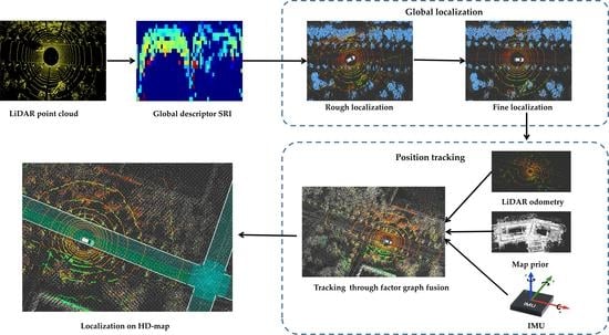
The localization methods we proposed are systematically introduced in this section. As shown in Figure 3, our localization algorithm includes four stages: (1) global descriptor generation stage, (2) global localization stage, (3) position tracking stage, and (4) HD map-based localization stage. The first stage is processed offline and the last three stages are processed in real time. Before these stages, we pre-build a point cloud map using the LiDAR inertial odometry via smoothing and mapping (LIO-SAM) [40] algorithm. In the first stage, we perform semantic segmentation on keyframes in the map to remove dynamic objects and encode the keyframes to generate the global descriptors SRI. In the second stage, the global descriptor generated in the previous stage is applied for global localization. The initial position of the targeted vehicle is obtained in the point cloud map by our global localization SRI-BBS, which is mainly divided into two parts: rough localization and fine localization. Then, our algorithm enters the third stage, the factor graph is considered to fuse LiDAR and IMU to track the position of the unmanned vehicle in the point cloud map. In the fourth stage, we mark on the point cloud map to generate an HD map, and using the localization result in the previous stage, we also achieve localization on an HD map.

3.1. Global Descriptor SRI

In this section, following the idea of coordinate removal and de-centralization we design a novel global descriptor SRI. This descriptor redefines its coordinate system through the distribution of the point cloud to improve its rotation invariance and shift invariance.

Firstly, in order to solve the problem that dynamic objects tend to change the point cloud and make global descriptors unstable, a lightweight deep learning model sparse point-voxel convolution with neural architecture search (SPVNAS) [41] is adopted to segment the point cloud semantically. In this paper, the parameters of SPVNAS are consistent with those of the original paper [41]. The process of SPVNAS is described in Appendix A. The current point cloud is defined as $P=\left\{p_1,p_2,\dots ,p_n\right\}$, and $p_i=\left\{x_i,y_i,z_i\right\}$ is defined as the coordinate value of the $i$th point in $P$. The cloud point $P$ processed by SPVNAS is as follows:

$$P^{\prime }=\left\{p_1^{\prime },p_2^{\prime },\dots ,p_n^{\prime }\right\}$$

(3)

$$p_i^{\prime }=\left\{x_i,y_i,z_i,labe{l}_i \right\}$$

(4)

where $P^{\prime }$ is the point cloud processed by SPVNAS, and $labe{l}_i$ is the semantic information of point $p_i^{\prime }$. The semantic information represents the classification of each point in the point cloud after semantic segmentation. It is defined as

Table 1. Definition of semantic information in point cloud.

1: car	2: bicycle	3: motorcycle	4: truck
5: other-vehicle	6: person	7: bicyclist	8: motorcyclist
9: road	10: parking	11: sidewalk	12: other-ground
13: building	14: fence	15: vegetation	16: trunk
17: terrain	18: pole	19: traffic-sign

from Sematic KITTI [42]:

The value of $labe{l}_i$ is an integer from 1 to 19. The points with $labe{l}_i$ from 1 to 8 belong to dynamic objects, such as vehicles and pedestrians, while the rest belong to static objects, such as building and sidewalk. Therefore, we can eliminate dynamic objects by removing the points defined by following formula:

$$p_i^{\prime }=\left\{x_i,y_i,z_i, labe{l}_i\right\},labe{l}_i<9.$$

(5)

Through the above process, the points with $labe{l}_i$ less than 9 are removed from the point cloud, and the rest of the points are retained in the point cloud. As shown in Figure 4a, we use different colors to visualize the semantic information of point clouds. The red points in the figure are vehicles, the green points are the roads, the blue and purple points are sidewalk and building, and the light blue points indicate fence. The result after removing the dynamic object is shown in Figure 4b. The red dynamic vehicle points were removed from the point cloud.

After the above preprocessing, we encode the point cloud to generate a rotation invariant and shift invariant descriptor. First, we calculate the covariance matrix of these points in the x, y dimensions by the following formula:

$$COV\left(X,Y\right)=\frac{1}{n-1}\left[\begin{array}{cc}{{\displaystyle \sum }}_{i=1}^n{\left(x_i-\overline{x}\right)}^2& {{\displaystyle \sum }}_{i=1}^n\left(x_i-\overline{x}\right)\left(y_i-\overline{y}\right)\\ {{\displaystyle \sum }}_{i=1}^n\left(x_i-\overline{x}\right)\left(y_i-\overline{y}\right)& {{\displaystyle \sum }}_{i=1}^n{\left(y_i-\overline{y}\right)}^2\end{array}\right]$$

(6)

where $X=\left\{x_1,x_2,\dots ,x_n\right\}$, $Y=\left\{y_1,y_2,\dots ,y_n\right\}$ represent the set of the point cloud on the x-axis and the y-axis, and$n$ is the number of its points. $COV\left(X,Y\right)$ is the covariance matrix of the point cloud in the x, y dimensions, and $\overline{x}$ and $\overline{y}$ are the mean values of $X$ and $Y$.

Next, two eigenvalues $e_1$, $e_2$ and two eigenvectors $v_1$, $v_2$ are calculated by singular value decomposition (SVD) of the covariance matrix $COV\left(X,Y\right)$. The eigenvector $v_2=\left(v_x,v_y\right)$ with larger eigenvalue is as the new x-axis direction, because the point cloud distribution in the frontal direction of larger eigenvalues is more dispersed and directional. When the distribution of the point cloud in the direction of the eigenvector becomes relatively uniform, its symmetry will result in both high levels of dispersions in the opposite two directions, which is prone to reversing the eigenvector by 180 degrees. To solve this problem, we calculate the angle between the eigenvector $\left(v_x,v_y\right)$ and the vector $\left(\overline{x},\overline{y}\right)$. If the angle is an obtuse one, $\left(v_x,v_y\right)$ is reversed, as shown in the following formula:

$$\stackrel{‵}{v_x}=\left\{\begin{array}{c}{v}_x, v_x·\overline{x}+v_y·\overline{y}\le 0\\ -v_x, v_x·\overline{x}+v_y·\overline{y}>0\end{array}\right. \stackrel{‵}{v_y}=\left\{\begin{array}{c}{v}_y, v_x·\overline{x}+v_y·\overline{y}\le 0\\ -v_y, v_x·\overline{x}+v_y·\overline{y}>0\end{array}\right.$$

(7)

where $\stackrel{‵}{v_x}$ and $\stackrel{‵}{v_y}$ are the reversing results. Then we set the $\left(\stackrel{‵}{v_x},\stackrel{‵}{v_y}\right)$ as the new x-axis and remap the point cloud onto the new coordinate system to provide rotation invariance, as shown in Formulas (8) and (9):

$$\theta =\arctan \left(\stackrel{‵}{v_y},\stackrel{‵}{v_x}\right)$$

(8)

$$\left[\begin{array}{c}{x}_i\\ y_i\\ z_i\end{array}\right]=\left[\begin{array}{ccc}\cos \theta & -\sin \theta & 0\\ \sin \theta & \cos \theta & 0\\ 0& 0& 1\end{array}\right]\left[\begin{array}{c}{x}_i\\ y_i\\ z_i\end{array}\right]$$

(9)

where $\theta$ is the angle between the main direction $\left(\stackrel{‵}{v_x},\stackrel{‵}{v_y}\right)$ and the positive direction of the x-axis, $x_i$,$y_i$, and $z_i$ are the coordinates of each point in the point cloud. Then we move the point cloud’s centroid $\left(\overline{x},\overline{y},\overline{z}\right)$ to the origin of the coordinates for providing the descriptor with shift invariance, as shown in following formula:

$$\left[\begin{array}{c}{\stackrel{‵}{x}}_i\\ {\stackrel{‵}{y}}_i\\ {\stackrel{‵}{z}}_i\end{array}\right]=\left[\begin{array}{c}{x}_i\\ y_i\\ z_i\end{array}\right]-\left[\begin{array}{c}\overline{x}\\ \overline{y}\\ \overline{z}\end{array}\right].$$

(10)

Finally, as shown in Figure 5, we divide the processed point cloud equally into ring along the radial direction and sector along the angular direction, resulting into $N_{ring}\times N_{sector}$ element regions, and $N_{ring}$ and $N_{sector}$ are the number of rows and columns, respectively. The row index $i$ and column index $j$ of the element region are calculated by following formula:

$$i=\left\{\begin{array}{c}\mathbf{\lceil }\frac{\arctan \left(\frac{x\left(p\right)}{y\left(p\right)}\right)+\frac{\pi }{2}}{2\pi }·N_{ring}\mathbf{\rceil }, 0<y\left(p\right)\\ \mathbf{\lceil }\frac{\arctan \left(\frac{x\left(p\right)}{y\left(p\right)}\right)+\frac{3\pi }{2}}{2\pi }·N_{ring}\mathbf{\rceil }, else\end{array}\right.$$

(11)

$$j=\mathbf{\lceil }\frac{RANGE+y\left(p\right)}{2·RANGE}\cdot N_{sector}\mathbf{\rceil }$$

(12)

where $p$ denotes a point of cloud point within the element region of the $i$th row and $j$th column, $x\left(p\right)$ and $y\left(p\right)$ represent the values of x-coordinate and y-coordinate about point $p$, respectively. $RANGE$ is the offset, which ensures the column index $j$ is a positive integer. In this paper, $N_{ring}=20$ and $N_{sector}=120$, which are set by experience. $RANGE=100$, which is determined by the maximum range of the LiDAR. Then, we take the maximum z value of each region to generate a $N_{ring}\times N_{sector}$ matrix as our global descriptor $M$, it can be defined by Formula (13):

$$M^{ij}=\underset{pϵR_{ij}}{\max }z\left(p\right)$$

(13)

where $M^{ij}$ is the value of row $i,$ column $j$ in descriptor $M$, and $z\left(·\right)$ is the function that returns the z-coordinate value of a point $p$. $R_{ij}=\left\{p_1,p_2,\dots ,p_m\right\}$ is the set of all points in the element region of the $i$th row and $j$th column, and $m$ is the number of points in $R_{ij}$. Then, the descriptor and the pose of its corresponding keyframe are recorded as $M=\left\{M_1,M_2,\dots ,M_n\right\}$ and $Q=\left\{Q_1,Q_2,\dots ,Q_n\right\}$, which are saved in a file for subsequent global localization.

3.2. SRI-BBS Global Localization Algorithm

In this section, we introduce our global localization algorithm SRI-BBS. Figure 6 shows the process of SRI-BBS, which is mainly divided into two parts: rough localization and fine localization. Rough localization is to obtain initial position information by searching the most similar map key frames with the SRI of current LiDAR scan. Fine localization dynamically selects a search range on the basis result of rough localization and uses the branch-and-bound scan matching algorithm [21] to obtain a more accurate position. It can make a trade-off between efficiency and precision. Rough localization costs less time. Its time complexity is $O\left(log n\right)$ and $n$ is the number of map keyframes. However, its result is approximate because the current position of the unmanned vehicle cannot be guaranteed to be exactly on the map keyframe. There is a certain rotation and translation between them. The time cost of fine localization is larger than rough localization because its time complexity is $O\left(\frac{R_{loc}}{∆x}·\frac{R_{loc}}{∆y}·\frac{360}{∆yaw}·log\left(\frac{R_{loc}}{∆x}·\frac{R_{loc}}{∆y}·\frac{360}{∆yaw}\right)\right)$. $R_{loc}$ is the search radius. $∆x$, $∆y$, and $∆yaw$ are the search steps in the x, y, yaw direction. However, its accuracy is higher than rough localization because all positions within the search range are searched at a certain search step. We can balance the time cost and accuracy by fine positioning on the basis of the rough localization result to achieve fast and accurate global localization. Finally, the NDT algorithm is used to verify whether global localization is successful. The process of NDT is described in Appendix B. The parameters of the NDT algorithm are referenced from the source code of HDL [22]: maximum iterations is 35, step size is 0.1, transformation epsilon is 0.01, and side length of the voxel grid is 1.0. Next, we will introduce the process of rough localization and fine localization in detail.

3.2.1. Rough Localization

The process of rough localization is shown in Figure 7. We first compute the current LiDAR scan into a descriptor $M$ using the method mentioned in Section 3.1. Then we compress the descriptor $M$ into a vector $V$, which contains $N_{ring}$ dimensions and is calculated by Formula (14):

$$V^i={\displaystyle \sum }_{j=1}^{N_{sector}}{M}^{ij}$$

(14)

where $V^i$ is the $i$-th dimension of vector $V$, $M^{ij}$ is the value of row $i,$ column $j$ in descriptor $M$, and $N_{sector}$ is the size of the column of descriptor $M$.

A KDTree containing all map keyframe vectors is established in advance in the map construction progress. We can speed up the retrieval process by KDTree. The time complexity of KDTree search is $O\left(log n\right)$. Then we search for $N_c$ candidates of map keyframes by KDTree; $n$ represents the number of map keyframes, and $N_c$ is set to 8. The position of these candidates is the most likely actual position of the current vehicle. Then the cosine distance is adopted to calculate the similarity between the SRI of current LiDAR scan and candidates, as shown in Formula (15):

$$sim=1-\frac{1}{N_{sector}}{\displaystyle \sum }_{i=1}^{N_{sector}}\frac{curSecto{r}_i·candSecto{r}_i}{\left|curSecto{r}_i\right|·\left|candSecto{r}_i\right|}$$

(15)

where $curSecto{r}_i$ represents the i-th column vector of the descriptor of the current frame, and $candSecto{r}_i$ represents the i-th column vector of the descriptor of the candidate frame. $N_{sector}$ represents the size of the column of the descriptor.

As shown in Algorithm 1, we find the most similar descriptor $M_S$ and its index $s$ among these $N_c$ candidates by using the similarity calculated in Formula (15). Since the index of the map’ descriptor and the index of the map keyframe are one-to-one correspondence, we can get the position of the map keyframe $P_s$ from the index $s$. Finally, we assign $Q_s$ to ($x_{init},y_{init},z_{init}$) as the result of rough localization.

Algorithm 1 Rough localization algorithm

Input: Current LiDAR scan $S$, Map descriptors set $M=\left\{M_1,M_2,\dots ,M_n\right\}$, map keyframe position set $Q=\left\{Q_1,Q_2,\dots ,Q_n\right\}$.

Output: Rough localization result $\{x_{init},y_{init},z_{init}\}$.

1: Compute current LiDAR scan $S$ to descriptor $D_c$ by method mentioned in Section 3.1; 2: Compress map descriptors $M$ into vectors V$=\left\{V_1,V_2,\dots ,V_n\right\}$ by Formula (14); 3: Compress descriptor $D_c$ into vector $V_c$ by Formula (14);

4: Use $V$ to build KDTree $T$; 5: $N_c$ candidate map descriptors that are most similar to $V_c$ are searched by KDTree $T$; 6: Find the most similar descriptor $M_S$ and its index $s$ among $N_c$candidate descriptors through the similarity calculated by Formula (15); 7: Get the position $Q_s=\{x_s,y_s,z_s\}$ of the map keyframe with index $s$; 8: $\{x_{init},y_{init},z_{init}\}=\{x_s,y_s,z_s\}$.

3.2.2. Fine Localization

After the rough localization, we next introduce the fine localization. As shown in Figure 8, we first convert the 3D point cloud map $H$ into a 2D binary grid map through the height threshold. It can be calculated as following formulas:

$$H=\underset{i\in \left\{1,2,\dots ,\lceil \frac{2E}{N_g}\rceil \right\},j\in \left\{1,2,\dots ,\lceil \frac{2E}{N_g}\rceil \right\}}{{\displaystyle \cup }}{G}_i^j$$

(16)

$$i=\mathbf{\lceil }\frac{E+x\left(p\right)}{N_g}\mathbf{\rceil }$$

(17)

$$j=\mathbf{\lceil }\frac{E+y\left(p\right)}{N_g}\mathbf{\rceil }$$

(18)

$$map\left(i,j\right)=\left\{\begin{array}{c}1, th\_min〈z_{ij} and th\_max〉z_{ij}\\ 0, else\end{array}\right.$$

(19)

where$i$ and$j$ represent the row index and column index of the grid map, respectively. $G_i^j$ is the set of the points within the grid of row $i$, column $j$, $p$ denotes a point of cloud point within the grid at row $i$ and column $j$, and $x\left(p\right)$ and $y\left(p\right)$ represent the values of x-coordinate and y-coordinate about point $p$. $E$ is the offset that ensures the row index $i$ and column index $j$ are positive integers. $N_g$ is the side length of the grid. The symbol $·$ indicates rounding up, $map\left(i,j\right)$ is the value of row $i$ and column $j$ in the grid map, $z_{ij}$ represents the maximum z-coordinate value of all points in $G_i^j$, $th\_min$ and $th\_max$ represent the minimum height threshold and maximum height threshold, respectively. In this paper, $E$ is set to 150, which is determined by the maximum range of the point cloud map. $N_g$ is set to 0.9, which is the appropriate grid size set by experience, $th\_\min =2$ and $th\_max$= 10, which are determined by the minimum and maximum heights of static objects within the point cloud map. Then, we generate a submap with lower resolution on the grid map by Formula (20).

$$Submap\left(i,j\right)=G\left(2i,2j\right)$$

(20)

where$Submap\left(i,j\right)$ is the value of row $i$ and column $j$ in the submap, $G\left(2i,2j\right)$ is the value of row $2i$ and column $2j$ in the grid map $G$. We can also generate a submap in the new submap by Formula (20). As show in Figure 9, we generate three submaps, each element of a submap consists of 0 or 1, the resolution of each layer is four times lower than that of the next layer.

After the above preprocessing, a search range around the rough localization result is dynamically selected via the descriptor similarity on the submap. This search range is a circle with ($x_{init},y_{init},z_{init}$) as the center and $R_{loc}$ as the radius. $R_{loc}$ is related to the similarity of descriptors calculated by Formula (21). As show in Figure 10, when the similarity of descriptor matching is high, the search range is reduced to improve the search efficiency, but not smaller than the threshold $R_{min}$; when the similarity is small, the search range is increased to improve the localization’s success rate, but not greater than the threshold $R_{max}$. In this paper, $R_{min}$ is set to 10 m, which is the minimum range of the map. $R_{max}$ is set to 100 m, which is determined by the maximum range of the LiDAR. $R_{loc}$ is calculated as follows:

$$R_{loc}=R_{min}+\left(R_{max}-R_{min}\right)·\left(1-Sigmoid\left(\left(sim-0.5\right)·k_r\right)\right)$$

(21)

where $sim$ is the similarity, the parameter 0.5 is to ensure that the value of $R_{loc}$ is between $R_{min}$ and $R_{max}$, and the calculation method of the Sigmoid function is:

$$Sigmoid\left(x\right)=\frac{1}{1+e^{-x}}$$

(22)

$k_r$ is the scale factor and $k_r$ > 0. The greater the $k_r$, the more sensitive the $R_{loc}$ is to the change in similarity. In this paper, $k_r$ is set to 8.

Finally, As shown in line 6 to 29 of the Algorithm 2, the branch-and-bound scan matching algorithm [21] is adopted within the search range $R_{loc}$ to obtain a more precise position. To show the details of our algorithm more clearly, the pseudo code of the fine localization algorithm is as follows:

Algorithm 2 Fine localization algorithm

Input: Rough localization result $\{x_{init},y_{init},z_{init}\}$, the similarity $s$ between the current frame descriptor and the most similar descriptor in the map descriptor set, the point cloud map $H$.

Output: Fine localization result $\{x_f,y_f,yaw\}$.

1:    Search range $R_{loc}$ is calculated by Formula (21); 2:    Convert point cloud map $H$ to 2d binary grid map $G$ by Formula (19); 3:    Convert LiDAR scan $S$ to 2d binary grid map $L$ by Formula (19); 4:    build three submaps $S=\{S_1,S_2,S_3\}$ in grid map $G$ by Formula (20); 5:    $best\_score$ ⟵ $score\_threshold$; 6:    Stack$C$ set to empty; 7:    for $x$ = $x_{init}$ − $R_{loc}$; $x$ < $x_{init}+R_{loc}$; $x$ = $x$ + $∆x$ do 8:   for $y$ = $y_{init}$ − $R_{loc}$; $y$ < $y_{init}+R_{loc}$; $y$ = $y$ + $∆y$ do 9:          for $yaw$ = $0$; $yaw$ < 360; $yaw$ = $yaw$ + $∆yaw$ do; 10:      Calculate the matching score under the poses $\left(x,y,yaw\right)$ in the lowest             resolution submap$S_1$, recorded as$\partial =\left(x,y,yaw,score,layer=1\right)$; 11:           Push $\partial$ to stack $C$; 12:      end for 13:    end for 14:    end for 15:    Sort stack $C$ by score, the maximum score at the top;

16:    while $C$ is not empty do; 17:       pop $c$ from the stack$C$; 18:       Current level $l\leftarrow c.layer$ on the submaps; 19:       if $c$.score > $best\_score$then 20:        if $l$ equals 3 then 21:         $best\_score$ ⟵$c$.score.\; 22:         $\{x_f,y_f,yaw\}$ ⟵ $\left\{ c.x, c.y, c.yaw\right\}$and break; 23:        else 24:         Branch: calculate the scores of four positions adjacent to current               position $c$on the higher resolution submap, recorded as              ${\epsilon }_1=\left(2c.x, 2c.y,c.yaw, scor{e}_1,c.layer+1\right)$,              ${\epsilon }_2=\left(2c.x+∆x/2^l, 2c.y,c.yaw, scor{e}_2,c.layer+1\right)$,              ${\epsilon }_3=\left(2c.x, 2 c.y+∆y/2^l,c.yaw, scor{e}_3,c.layer+1\right)$,              ${\epsilon }_4=\left(2c.x +∆x/2^l,2c.y+∆y/2^l, c.yaw, scor{e}_4, c.layer+1\right)$; 25:         Push ${\epsilon }_1, {\epsilon }_2, {\epsilon }_3, {\epsilon }_4$ onto the stack C, sorted by score, the maximum score at the top; 26:        end if 27:       end if 28:    end while 29:    return $\{x_f,y_f,yaw\}$.

In the pseudo code, $Score\_threshold$ in the code is set to 130, which determines the minimum score when our algorithm converges. The method to calculate the matching score in the 10th and 24th lines of code are calculated as follows:

$$Score={\displaystyle \sum }_{i=0}^r{\displaystyle \sum }_{j=0}^q{L}^{ij}\oplus S^{ij}$$

(23)

where $L$ is the grid map of the current LiDAR scan, $L^{ij}$ is the pixel value of row $i,$ column $j$ in $L$, and $S$ is the current submap. $S^{ij}$ is the pixel value that the pixel of $L^{ij}$ overlaps in the submap $S$, and $\oplus$ is xor operation; $r$, $q$ is the row and column size of $L$, respectively. The calculation step of lines 6 to 15 is to enumerate all poses with step size $∆x$, $∆y$, and $∆yaw$, respectively, within $R_{loc}$ on the submap with the lowest resolution. Then, the matching scores are calculated under these poses. $∆x$, $∆y$, and $∆yaw$ are set to 0.3, 0.3, and 0.5, which are obtained as a trade-off between time efficiency and accuracy. Additionally, $layer$ and $l$ indicate the level of submaps. Lines 16 to 28 show the process of the branch-and-bound scan matching algorithm: depth first search (DFS) is used to find the optimal solution. We search four positions adjacent to current position of $c$on the submap with higher resolution during branching. Since the resolution of the next layer of the submap is four times of the previous layer, these four positions are in $\left(2c.x, 2c.y\right)$, $\left(2c.x+∆x/2^l, 2c.y\right)$, $\left(2c.x, 2c.y+∆y/2^l\right)$, and $\left(2c.x+∆x/2^l, 2c.y+∆y/2^l\right)$. When calculating the bounds on the subsets, the number of submap layers is set to 3, and only four adjacent points are searched to determine the bounds. When the matching score is greater than $score\_threshold$ and the current layer is the submap with the highest resolution, our algorithm converges and the fine localization result is returned.

3.3. Position Tracking Algorithm

After global localization, we initialized the pose of the unmanned vehicle in the map. As shown in Figure 11, with the movement of the unmanned vehicle, we fuse the measurements of LiDAR, IMU, and map’s prior information to estimate the pose of the unmanned vehicle in real time for position tracking. The relative motion between LiDAR frames can be obtained by LiDAR odometry, and the higher frequency motion estimation can be obtained by integrating IMU measurement. In our position tracking algorithm, we apply the Georgia Tech smoothing and mapping library (GTSAM) [12] to establish a tightly coupled factor graph model to estimate the pose of unmanned vehicles in real time. The structure of the factor graph model is shown in Figure 12. This factor graph can integrate LiDAR odometry, IMU pre-integration, and the map prior. The LiDAR odometry and IMU pre-integration are as binary edges in the factor graph, and the map prior is as a unitary edge in the factor graph. After factor graph fusion, we can obtain more stable and robust position tracking results.

The LiDAR odometry is applied with LOAM. We assume the uniform motion model of the unmanned vehicle, as shown in the following formula:

$$x_i=x_{i-1}+v·∆t$$

(24)

where $x_i$ is the pose at current time, $x_{i-1}$ is the pose at the last time, and $v$ is the velocity, which can be obtained by dividing the transformation of the pose by the interval time.

The map prior is calculated by the NDT method and its detailed procedure is described in Appendix B. We set the parameters of the NDT as follows: maximum iterations is 15, step size is 0.1, transformation epsilon is 0.01, and side length of voxel grid is 1.0.

The measurement model of IMU pre-integration is as follows:

$$R\left(t+∆t\right)=R\left(t\right)·Exp\left(\omega \left(t\right)·∆t\right)$$

(25)

$$V\left(t+∆t\right)=V\left(t\right)+a^w\left(t\right)·∆t$$

(26)

$$P\left(t+∆t\right)=P\left(t\right)+V\left(t\right)·∆t+\frac{1}{2}{a}^w\left(t\right)·∆t^2$$

(27)

where $∆t$ is a tiny interval, $R\left(t\right)$ represents the rotation matrix at time$t$, $\omega \left(t\right)$ is the angular velocity of IMU at time $t$, $V\left(t\right)$ is the velocity at time $t$, $a^w\left(t\right)$ is the accelerated velocity of unmanned vehicle at time $t$ measured by IMU, and $P\left(t\right)$ is the position at time $t$. We can get the angle by integrating the angular velocities, obtain the linear velocity by integrating the acceleration, and obtain the displacement by integrating the linear velocities. The uncertainty of the motion model is stable in translation, but high in rotation. However, the uncertainty of IMU measurement in rotation is lower than that of motion model. Especially when the unmanned vehicle is rotating rapidly, the IMU measurement in rotation can provide good robustness for position tracking.

Next, the cost function from incremental smoothing and mapping using the Bayes tree (ISAM2) [12] is used in our factor graph model. It is defined as Formula (28):

$$F\left(\tau \right)={\displaystyle \sum }_i{e}_i^T{\Omega }_i{e}_i+{\displaystyle \sum }_{ij}{e}_{ij}^T{\Omega }_{ij}^L{e}_{ij}+{\displaystyle \sum }_{ij}{\stackrel{‵}{e}}_{ij}^T{\Omega }_{ij}^I{\stackrel{‵}{e}}_{ij}$$

(28)

$$e_i={\tau }_i-z_i$$

(29)

$$e_{ij}={\tau }_j-{\tau }_i-o_{ij}$$

(30)

$${\stackrel{‵}{e}}_{ij}={\tau }_j-{\tau }_i-I_{ij}$$

(31)

where $\tau =\left\{{\tau }_1,{\tau }_2,\dots ,{\tau }_n\right\}$ is the set of pose of all nodes in the factor graph, $n$ is the number of nodes in the factor graph, ${\tau }_i=\left(x_i,y_i,z_i,rol{l}_i,pitc{h}_i,ya{w}_i\right)$ is the pose of the $i$th node in $\tau$, $e_i$ is the unary edge residual of the map’s prior information, defined by Formula (29), $z_i=\left(\stackrel{‵}{x_i},\stackrel{‵}{y_i},\stackrel{‵}{z_i},\stackrel{‵}{rol{l}_i},\stackrel{‵}{pitc{h}_i},\stackrel{‵}{ya{w}_i}\right)$ is the measurement of the map prior, and $e_{ij}$ is the binary edge residual of the LiDAR odometry in the factor graph, defined by Formula (30). Additionally, $o_{ij}=\left(x_{ij},y_{ij},z_{ij},rol{l}_{ij},pitc{h}_{ij},ya{w}_{ij}\right)$ is the measurement of the LiDAR odometry between $i$th and $j$th nodes of the factor graph, ${\stackrel{‵}{e}}_{ij}$ is the binary edge residual of the IMU pre-integration in the factor graph, defined by Formula (31). $I_{ij}=\left({\stackrel{‵}{x}}_{ij},{\stackrel{‵}{y}}_{ij},{\stackrel{‵}{z}}_{ij},{\stackrel{‵}{roll}}_{ij},{\stackrel{‵}{pitch}}_{ij},{\stackrel{‵}{yaw}}_{ij}\right)$ is the measurement of the IMU pre-integration between $i$th and $j$th nodes of the factor graph, ${\Omega }_i$, ${\Omega }_{ij}^L$, and ${\Omega }_{ij}^I$ are the information matrices of map prior, LiDAR odometry and IMU pre-integration, respectively.

The values of the information matrix are referenced from the source code of LIO-SAM [40]. The information matrix provides different weights for residuals of the map prior, LiDAR odometry, and IMU pre-integration. Its value is only related to the measurement accuracy of the sensor and is independent of the application scenario. The measurement with higher accuracy is set with greater weight, while the measurement with lower accuracy is set with lower weight. Therefore, ${\Omega }_i$ is set as a 6 * 6 matrix with ${10}^{-4}$, ${10}^{-4}$, ${10}^{-4}$, ${10}^{-4}$, ${10}^{-4}$, and ${10}^{-4}$ on the diagonal, and the rest are all 0. Additionally, ${\Omega }_{ij}^L$is set as a 6 * 6 matrix with ${10}^{-3}$, ${10}^{-3}$, ${10}^{-3}$, ${10}^{-5}$, ${10}^{-5}$, and ${10}^{-5}$ on the diagonal, and the rest are all 0; ${\Omega }_{ij}^I$is set as a 6 * 6 matrix with ${10}^{-5}$, ${10}^{-5}$, ${10}^{-5}$, ${10}^{-3}$, ${10}^{-3}$, and ${10}^{-3}$ on the diagonal, and the rest are all 0. Next, the Levenberg–Marquardt method is adopted to minimize the cost function to obtain the optimally estimated pose $\tau$. The calculation formula is as follows:

$${\tau }^{\ast }=\arg \underset{\tau }{\min }F\left(\tau \right)$$

(32)

where $\tau$ is the pose to optimize, including x, y, z, roll, pitch, and yaw. We set the number of iterations for Levenberg–Marquardt optimization to 15.

Finally, we apply a grid-based algorithm for local map update to expedite the tracking process. First, we divide the point cloud map into multiple 30 m × 30 m grids, as shown by the grids cut with the yellow lines in Figure 13. Additionally, the white part in the figure is the global point cloud map, and the colorful highlighted rectangular area is the local map. We record the range of each grid point $\left\{x_{grid\_min},x_{grid\_max},y_{grid\_min},y_{grid\_max}\right\}$, where $x_{grid\_min}$ is the minimum value of x in the grids, $x_{grid\_max}$ is the maximum value of x in the grids, $y_{grid\_min}$ is the minimum value of y in the grids, and $y_{grid\_max}$ is the maximum value of y in the grids. We expedite the updating of local maps by first selecting the grid then the map points within the grids. During the process of grid selection, for the grid that we search intersecting with the local map, we need to make a judgment on whether each point in the grid falls within the local map. If so, we can add this point into the local map; if not, we shall not add it. For the grid that we search not intersecting with the local map where $x_{min}<x_{grid\_min}$ or $x_{max}>x_{grid\_max}$ or $y_{min}<y_{grid\_min}$ or $y_{max}>y_{grid\_max}$, we will directly skip the grid without further judgment about whether its points are in the local map or not, so as to expedite the update of the local map. It is essentially a method of exchanging space for time.

3.4. HD Map Localization

Because the point cloud map cannot provide effective auxiliary information of road networks for navigation and planning, we adopt the Roadrunner tool to mark the point cloud map to generate an HD map that applies the Apollo OpenDRIVE format. We design and implement an HD map engine, which can realize the lane-level localization, and provide the current lane information of the unmanned vehicle and its specific position on this lane. The engine can also search other map information, such as the intersection information, road topology, stop line, etc.

To quickly search the lane of the unmanned vehicle, we design a lane-level localization algorithm. In the OpenDRIVE format, each lane has a virtual central line consisting of dispersed points. We adopt the KDTree algorithm to search the m candidate lanes closest to the targeted vehicle’s position. In this paper, the data size of m is set to 4. Hypothesizing that the current localization coordinate of the unmanned is $\left(x_{loc},y_{loc}\right)$, we can determine whether it is in one of the candidate lanes through the point inclusion in polygon (PNPoly) [43] algorithm to find the lane where the unmanned vehicle is on. The algorithm for calculating the current lane of the unmanned vehicle is as follows:

As listed in Algorithm 3, the second line searches the $m$ candidate lanes closest to the vehicle position ($x_{loc},y_{loc}$) through the KDTree algorithm, and the fourth to twelfth lines judge whether the current position of the unmanned vehicle falls within the candidate lane through the PNPoly algorithm. If so, it will directly retrieve the lane’s information, and if not, it will move to judge the next candidate lane.

Algorithm 3 lane-level localization algorithm

Input:

Localization position $\left(x_{loc},y_{loc}\right)$, lane sets of HD map

Output:

Current lane information $L_{cur}$

Algorithm:

1:    Begin:

2:     KDTree algorithm searches the m candidate lanes nearest to $\left(x_{loc},y_{loc}\right)$

3:     for each lane $L_i$ in candidate lanes do 4:       is_in $\leftarrow$ False

5:       for each edge in $L_i$ do

6:          if edge intersects the ray $y = y_{loc}$ then

7:                is_in $\leftarrow$!is_in

8:          end if

9:       end for

10:        if is_in equals True then

11:           return the lane information of $L_i$

12:        end if

13:      end for

14:      return not in any lane

15: end begin.

Figure 14 is the schematic diagram of our lane model. The calculation of the position of the unmanned vehicle within the lane is exactly the process of calculating the $s$ and $t$ marked in the figure; $s$ is the longitudinal distance along the lane and $t$ is the lateral distance from the central line of the lane, and $s$ can be acquired by integrating the distances of adjacent points on the central line, as shown in Formula (33):

$$s={\displaystyle \sum }_{i=2}^j\sqrt{{(x_i-x_{i-1})}^2+{\left(y_i-y_{i-1}\right)}^2}$$

(33)

where j represents the index of the point closest to the unmanned vehicle, $x_i$ represents the abscissa of the i-th point on the central line, and $y_i$ represents its ordinate.

The calculation of $t$ is shown in Formula (34):

$$t=\sqrt{{\left(x_c-x_{loc}\right)}^2+{\left(y_c-y_{loc}\right)}^2}$$

(34)

where $x_c$ represents the abscissa of the central line point closest to the unmanned vehicle, and $y_c$ represents its ordinate. The sign of $t$ depends on the distance between the unmanned vehicle and the left/right boundaries. If it is close to the left boundary, the sign will be positive, and if it is close to the right boundary, the sign will be negative.

4. Experiments

In this section, we validate the proposed algorithm on the KITTI benchmark dataset and the actual data scenario of the Jilin University campus. First, two ablation experiments are conducted to guarantee the effectiveness of the global descriptor and dynamic range search strategy. Secondly, our global localization algorithm SRI-BSS is compared with the opensource algorithm scan context [10] and the global localization algorithm of HDL [22]. Then we perform an ablation experiment to verify that our factor graph model can improve the performance of position tracking. Furthermore, we contrast our tracking algorithm separately with the HDL and NDT [34] to prove that our algorithm achieved the performance of the current mainstream algorithms. Finally, we mark the effect of lane-level localization on the HD map. The above experiments were implemented on a machine with the CPU of Intel Xeon E5-2607, 2.6 G Hz frequency, the memory of 32 G, and the GPU of GTX Titan X.

4.1. Dataset Introduction

4.1.1. KITTI Dataset

KITTI is a classic and well-known benchmark dataset, being applied in visual odometry, SLAM, and localization tasks. We performed the experiments on the KITTI benchmark sequences of 00, 01, 02, 04, 05, 06, 07, 08, 09, and 10, respectively. The specifics of KITTI dataset are listed in

Table 2. KITTI dataset specifics.

Sequence	Scans	Trajectory Length (m)	Proportion of Frames Containing Dynamic Items
00	4541	3722	32%
01	1101	2588	13%
02	4661	5067	26%
04	271	403	16%
05	2761	2206	24%
06	1101	1220	17%
07	1101	694	28%
08	5171	2631	21%
09	1591	1709	16%
10	1201	919	12%

.

4.1.2. JLU Campus Dataset

The JLUROBOT team owns multiple data collecting platforms applicable for the data collection, mapping, and localization tasks under different road conditions. Figure 15 displays some of the collection platforms, among which the J5 collection platform is adopted for data constructions in mountains and forests, while the Avenger collection platform is appropriate for data constructions in off-road environments. The JLU campus dataset is collected on the campus of Jilin University by the Volkswagen Tiguan data collection platform. As shown in Figure 16, this mobile platform is equipped with the Velodyne HDL-32E surround LiDAR sensor to collect the point cloud data, and the NPOS220S inertial navigation system (INS) to acquire ground truth, acceleration speed, and angular velocity information.

The JLU campus dataset consists of 11 data series. One of these is used for mapping and the total length of the road is 3722 m. The proportion of frames containing dynamic items is 27%. Using the above data, a point cloud map, as shown in Figure 17a, was constructed by the LIO-SAM method with the trajectory shown as the blue line in Figure 17b. The RTK-GNSS is adopted during the mapping process. The average precision error of the generated global map is 10 cm. The remaining 10 sequences are the testing data, where the total road length of JLU_01 are 3947 m and the trajectory is generally consistent with the previous data sequences. When the test positioning points are not on the mapped trajectory, some locations are locally changed to test the effect, and their trajectories are shown in red in Figure 17b. The JLU_02 to JLU_10 are nine sequences of data randomly collected on the mapping data path.

4.2. Global Localization Experiments

In this section, we first complete two ablation experiments to verify the performance of our global descriptor SRI and our SRI-BBS, respectively. Secondly, we also complete a comparative experiment to prove that the comprehensive performance of our global localization algorithm reached the mainstream algorithms. In the first ablation experiment, we adopt the control variable method to verify that our descriptor SRI has excellent rotation invariance and shift invariance by replacing the descriptor with scan context and keeping the other parts unchanged. In the second ablation experiment, we change the search range from a dynamic value to a fixed value of 130 to verify that the SRI-BBS global localization algorithm can improve the efficiency and success rate of localization. In the comparative experiment, we compare our global localization algorithm with the opensource algorithms scan context and HDL to verify that our algorithm achieves the performance of the current mainstream algorithms.

4.2.1. Ablation Experiments of Global Descriptor

We adopt the control variable method to conduct the experiments to verify that our global descriptor SRI has excellent rotation invariance and shift invariance. We replace the SRI descriptor in SRI-BBS with the scan context [10] descriptor, named SC-BBS, and keep other parts unchanged. Firstly, we conducted the ablation experiments of global localization on the KITTI dataset. Because each sequence of the KITTI dataset contains only one piece of data, its testing will be meaningless if the data are applied for both mapping and localization. Therefore, our strategy was to select one map key frame for every five frames of the point cloud for mapping and the rest for global localization during the mapping process. The local map searched by global localization will be registered by NDT with the point cloud participating in this search, then determines whether the localization is successful based on the NDT’s fitness score. When the fitness score is less than 2, the localization is judged to be successful, otherwise it is judged to be a failure. Then, we calculate the success rate of the global localization algorithm by the following formula:

$$p=\frac{S}{S+F}$$

(35)

where $p$ represents the success rate, $S$ represents the number of point cloud frames successfully localized, and $F$ represents the number of failed frames.

As can be seen in the left half of

Table 3. Ablation experiment results in global descriptors in the KITTI and JLU campus datasets.

KITTI Dataset			JLU Campus Dataset
Sequence	SC-BBS	Ours	Sequence	SC-BBS	Ours
00	95.3%	97.3%	JLU_01	90.3%	98.7%
01	88.2%	91.6%	JLU_02	95.2%	97.6%
02	86.2%	90.7%	JLU_03	94.6%	99.4%
04	95.1%	86.2%	JLU_04	94.2%	98.2%
05	83.6%	97.8%	JLU_05	90.5%	97.8%
06	86.6%	98.8%	JLU_06	93.3%	99.1%
07	96.8%	98.4%	JLU_07	92.4%	97.4%
08	96.5%	96.9%	JLU_08	81.2%	97.9%
09	92.1%	93.7%	JLU_09	86.7%	86.0%
10	86.6%	87.4%	JLU_10	92.1%	90.1%
Average	90.7%	93.9%	Average	91.0%	96.2%

Notes: The bold numbers indicate the best results.

, the success rate of our localization algorithm is significantly higher than that of SC-BBS for the 10 sequences of KITTI data, except for the 04 sequence. The average success rate of SC-BBS’ global localization on these 10 segments of data is 90.7%, while the rate of our algorithm is 93.9%. Results effectively indicate that the performance of the global descriptor proposed in this paper is superior to that of scan context, mainly because scan context has no shift invariance. When the localization point is between the keyframes, the relative position change of the object in the point cloud imposes a great impact on scan context, resulting in scan context mismatch and localization failure. Our algorithm enhanced the shift invariance of descriptors through decentralization. Though the current position is not on the map keyframes, we can still find the map keyframes are close to them to some extent. Furthermore, the proposed method did not work well on the 04 sequence, probably because this sequence of data is relatively short with only 271 frames of data. Our mapping strategy is to select a keyframe every five frames to participate in the mapping, so it appears somewhat fortuitous that the point cloud data for sequence 04 is small, which is involved in the mapping match. Consequently, the indication value of the results of this segment is quite limited.

We also conducted the same ablation experiments on the JLU campus dataset to further validate the effectiveness of our proposed descriptor SRI in real scenarios. According to Table 3, the average success rate of our algorithm is 5.2% higher than that of SC-BBS, and the advantage of our algorithm can be best demonstrated on JLU_01. As can be seen from Figure 17b, there is a section of JLU_01 where the localization points are not on the mapped trajectory. Specifically, the success rate of our algorithm on JLU_01 is 98.7%, which is higher than the 90.3% of SC-BBS. For these localization points, as scan context has no shift invariants, the descriptor indication on the local mapping trajectory in the localization region will become irrelevant and SC-BBS will be prone to mismatch these localization points with other key frames in the mapping trajectory, leading to localization failure.

Figure 18 exhibits the individual effects of the above two global localization methods. As can be seen, the green short lines indicate locations where localization is successful and the short red lines indicate locations where localization fails. In Figure 18, we also adopt the yellow circles to indicate four areas with significant differences in the localization results, and mark them with a, b, c, and d, respectively. These positions are all within the range of the constructed map, but they are at a certain distance from the blue mapping trajectory. Point a and point b are both positioned in the car park in front of the computer building at Jilin University, the localization trajectory and mapping trajectory are two parallel lanes in the parking lot, with an interval of 4 m. Comparing the upper right parts of point a in these two figures, we can see that our method has more short lines with green and less red short lines than SC-BBS, demonstrating that the descriptor proposed exerts a better matching effect in the case of obvious shifts between the localization points and the mapping trajectory, with a certain level of shift invariance. For points c and d, there is not only a larger level of shifts, but also a rotation change contrasted to the mapping trajectory compared with points a and b. Our method presents a higher localization success rate than SC-BBS, reflecting that the SC-BBS method has more points of failed localization. By comparing these ablation experiments of the above specific roads, it is illustrated that our descriptor is not only better in tackling the shift problem, but also effective in addressing the rotation problem.

4.2.2. Ablation Experiments of SRI-BBS Global Localization

To verify that our tracking algorithm can improve the success rate and time efficiency of global localization, we perform a round of ablation experiments. In this round of ablation experiments, we change the search range $R_{loc}$ in SRI-BBS from a dynamic value to a fixed value of 130, and the other configurations keep unchanged. We name this method SRI-STATIC to be compared with SRI-BBS. We test it on the KITTI and JLU campus datasets, using the same method in Section 4.2.1, respectively. As a result,

Table 4. Ablation experiment results of SRI-BBS in the KITTI dataset and JLU campus dataset.

KITTI Dataset			JLU Campus Dataset
Sequence	SRI-STATIC	Ours	Sequence	SRI-STATIC	Ours
00	4693	535	JLU_01	4286	521
01	5782	582	JLU_02	4597	593
02	4894	636	JLU_03	5317	564
04	5217	488	JLU_04	5188	492
05	5792	538	JLU_05	4197	581
06	4831	543	JLU_06	4731	539
07	4937	528	JLU_07	5873	499
08	5274	615	JLU_08	4258	521
09	5931	620	JLU_09	4364	578
10	5241	539	JLU_10	4821	565
Average	5259	562	Average	4763	545

Notes: The unit of time consumption is milliseconds. The bold numbers indicate the best results.

and

Table 5. Success rates of SRI-BBS’ ablation experiments under KITTI dataset and JLU campus dataset.

KITTI Dataset			JLU Campus Dataset
Sequence	SRI-STATIC	Ours	Sequence	SRI-STATIC	Ours
00	93.6%	97.3%	JLU_01	92.4%	98.7%
01	91.5%	91.6%	JLU_02	93.7%	97.6%
02	86.2%	90.7%	JLU_03	91.6%	99.4%
04	95.1%	86.2%	JLU_04	93.1%	98.2%
05	93.6%	97.8%	JLU_05	90.7%	97.8%
06	92.4%	98.8%	JLU_06	92.6%	99.1%
07	94.8%	98.4%	JLU_07	91.3%	97.4%
08	92.1%	96.9%	JLU_08	88.6%	97.9%
09	93.7%	93.7%	JLU_09	86.7%	86.0%
10	84.2%	87.4%	JLU_10	89.4%	90.1%
Average	91.7%	93.9%	Average	91.0%	96.2%

Notes: The bold numbers indicate the best results.

present the time consumption and localization success rates on these two datasets. We test it on the KITTI and JLU campus datasets, using the same method in Section 4.2.1, respectively. As a result, Table 4 and Table 5 present the time consumption and localization success rates on these two datasets.

As can be seen from Table 4, the average time taken for a single frame on the KITTI dataset is 562 ms for our method and 5259 ms for the SRI-STATIC method. On the JLU campus dataset, the average time taken for a single frame for the SRI-STATIC method is 4763 ms, which is clearly higher than the 545 ms for our method. The main reason is that we use the similarity of SRI to acquire the search range dynamically. When the similarity is high, we do not need to search a larger space. By narrowing the search range, the search time consumption can be reduced. The performance on the JLU campus dataset also reflects the good generalization capability of our method and its ability to achieve global localization quickly.

Table 5 lists the global localization success rates of above two methods on KITTI and JLU campus, respectively. Both on the KITTI and SRI-STATIC dataset, the average localization success rate is higher than SRI-STATIC. It effectively indicated that in the process of narrowing the search range, the proposed method also reduced the impacts of interference points in the map on the matching algorithm. Furthermore, we visually displayed the matching process of point clouds within a dynamic range and fixed range to further illustrate the effectiveness. Figure 19 shows the matching ranges selected by two different methods at positions of a, b, and c. The SRI-STATIC algorithm will consider the red area when calculating the vehicle positions, leading to localization failures. However, the search area of our algorithm is only a small part of the circular blue area, and there will be no data from other positions involved in the calculation of the final result in the matching process. In this case, our localization algorithm adopted a dynamic search strategy: when the descriptors of current frame and map keyframe were highly similar to each other, we narrowed the search range to exclude the points in the red box and skillfully avoid these interference points. The visualized results show that the dynamic range selection method proposed in this paper could effectively avoid the occurrence of some mismatching. Figure 20 exhibits the actual localization effect of the global localization algorithm proposed in this paper at different positions in the map of Jilin University. Our unmanned vehicle was successfully initialized onto the map.

4.2.3. Comparative Experiments of Global Localization

We further compared the proposed global localization algorithm SRI-BBS with the open-source algorithms scan context [10] and HDL [22] on KITTI and JLU campus datasets under the same machine configuration. We set the number of iterations of all algorithms to 15. For comparison with scan context descriptors, we used NDT for scan-to- map alignment during the matching process, called SC-NDT. We scored how well the point cloud matched the map to determine whether the localization was successful. In the mapping process, we select a map key frame from every five frames and use the rest of the data for localization. Through the above operation, the mapping data and positioning data do not overlap, both to achieve the difference between experimental and test data, and to verify whether the global positioning is successful when the initial position of the unmanned vehicle is between the keyframes of the map.

According to

Table 6. Comparative experiment results under the KITTI dataset and JLU campus dataset.

KITTI Dataset				JLU Campus Dataset
Sequence	SC-NDT	HDL	Ours	Sequence	SC-NDT	HDL	Ours
00	77.3%	75.8%	97.3%	JLU_01	47.5%	95.3%	98.7%
01	74.0%	79.5%	91.6%	JLU_02	52.4%	88.2%	97.6%
02	76.2%	65.8%	90.7%	JLU_03	49.5%	86.2%	99.4%
04	84.9%	86.8%	86.2%	JLU_04	46.8%	95.1%	98.2%
05	82.8%	78.5%	97.8%	JLU_05	53.6%	83.6%	97.8%
06	68.1%	83.6%	98.8%	JLU_06	48.5%	86.6%	99.1%
07	75.0%	72.9%	98.4%	JLU_07	50.3%	96.8%	97.4%
08	63.8%	76.7%	96.9%	JLU_08	45.9%	96.5%	97.9%
09	81.4%	84.8%	93.7%	JLU_09	43.7%	92.1%	86.0%
10	76.3%	89.3%	87.4%	JLU_10	52.4%	86.6%	90.1%
Average	76.0%	79.4%	93.9%	Average	49.1%	90.1%	96.2%

Notes: The bold numbers indicate the best results.

, the average success rate of the global localization algorithm proposed in this paper is 93.9% on the KITTI dataset, which is 17.9% higher than the SC-NDT method and 14.5% higher than the HDL method. However, in sequences 04 and 10, the success rate of the method is slightly lower than that of the HDL method. The main reasons for this are the shorter length of these two sequences, the simplicity of the trajectories, the absence of closed loops, the small amount of map data generated and the small number of similar scenes. In addition, HDL obtains the best pose by exhausting x, y, and yaw in a multi-resolution mapping, which is considered an exhaustive search method, but is very effective in this simple small scene type.

We also conducted comparative experiments with SC-NDT and HDL on the JLU campus dataset to validate the effectiveness of our global localization algorithm in real-life scenarios. The experimental results show that our global localization algorithm achieves an average success rate of 96.2% in real campus scenarios, which exceeds the 49.1% of SC-NDT and 90.1% of HDL. It can be seen that the proposed algorithm has a good generalization capability. We also counted the proportional distribution of the distance from the localization point to the map keyframe in the JLU campus dataset and analyzed the relationship between the distance from the localization point to the map keyframe and the localization success rate, as shown in Figure 21 below:

Figure 22 exhibits the proportional distribution of the distances from the initial position of the unmanned vehicle to the mapping trajectory. The red polyline exhibits the success rates of our algorithm at different distances. The green polyline displays the success rates of the SC-NDT algorithm at different distances. The orange polyline presents the success rates of the HDL algorithm at different distances. Our polyline is generally above the green and the orange ones, which indicates that our global localization algorithm has a higher localization success rate than both SC-NDT and HDL. When the distance grows beyond 8 m, SC-NDT is unable to localize any more. This is because although scan context has certain rotation invariance, it does not have shift invariance. When the localization point is beyond a specified distance from the map keyframes, it will be difficult to estimate the priori pose. HDL method is an exhaustive matching search, hence when the scenario grows larger and the number of similar scenarios increases, its effect will significantly decline. However, our localization algorithm SRI-BBS adopts our global descriptor SRI, which remaps the point cloud to achieve certain levels of shift invariance and rotation invariance. Even if the localization point is at a certain distance from the map keyframes, we can still find the ones nearby as priori pose information. Secondly, according to the similarity of descriptors, we dynamically select the search range and branch-and-bound scan matching to find the more accurate position.

As shown in Figure 22, it shows a case of our global localization algorithm under the JLU campus dataset. The point cloud collected by the LiDAR is semantically segmented and then encoded into a global descriptor SRI. KDTree is used to search for eight candidates map’s global descriptors. Then, the most similar candidate descriptor is selected to perform rough localization. The blue points in the rough and fine localization are the point cloud map, and the other color points are the current LiDAR scan. Finally, a more accurate pose is obtained by performing fine localization.

4.3. Position Tracking Experiments

In this section, we complete an ablation experiment and a comparative experiment to verify the performance of our factor graph model and position tracking algorithm, respectively. In the ablation experiment, we adopt the control variable method to verify that our factor graph model can improve the localization accuracy by removing the factor graph part and keeping the rest unchanged. In the comparative experiment, we compare our position tracking algorithm with HDL and NDT to verify that our position tracking algorithm achieves the performance of the current mainstream algorithms.

4.3.1. Ablation Experiments of Position Tracking

The control variable method is adopted to verify that our factor graph model can improve the performance of position tracking. We remove the factor graph model and keep the remaining part unchanged, and then compare the results obtained by scan-to-map for ablation experiments on the KITTI dataset and the JLU campus dataset. We adopt the GNSS data as the ground truth to evaluate the precision of the results of the proposed algorithm. The following formula can calculate the localization error:

$$e\left(t\right)=\sqrt{e_x{\left(t\right)}^2+e_y{\left(t\right)}^2}$$

(36)

where $e_x\left(t\right)$ and $e_y\left(t\right)$ are individually the errors between the localization results and the ground truth of GNSS on the x-axis and y-axis.

Table 7. Ablation experiment results in position tracking under the KITTI and JLU campus datasets.

KITTI Dataset			JLU Campus Dataset
Sequence	No Factor Graph Model	Ours	Sequence	No Factor Graph Model	Ours
0	0.316	0.224	JLU_01	0.382	0.272
1	0.295	0.141	JLU_02	0.261	0.14
2	0.342	0.281	JLU_03	0.352	0.199
4	0.154	0.096	JLU_04	0.247	0.218
5	0.231	0.141	JLU_05	0.413	0.246
6	0.286	0.277	JLU_06	0.196	0.178
7	0.273	0.266	JLU_07	0.341	0.293
8	0.258	0.218	JLU_08	0.472	0.352
9	0.225	0.151	JLU_09	0.394	0.389
10	0.137	0.117	JLU_10	0.286	0.264
Average	0.252	0.191	Average	0.334	0.253

Notes: The bold numbers indicate the best results. The unit of localization error is meter.

shows the localization errors of the ablation experiments on the KITTI dataset and the JLU campus dataset. It is obvious that the average error of our algorithm is 0.061 m lower than that of the no factor graph model in the KITTI dataset. At the same time, the localization error of our algorithm under the JLU campus dataset is 0.081 m lower than that of the no factor graph model. This is because the control group only uses scan-to-map to obtain map priori information, which does not converge well when the vehicle is moving rapidly or making fast turns. In our algorithm, we use the factor graph model to integrate the LiDAR odometry, IMU pre-integration, and map prior. It solves the limitations of a single sensor in these situations, which can greatly improve the robustness of the algorithm. Figure 23 shows the localization trajectory under the JLU campus dataset’s sequence 01. The blue line is our algorithm, and the green line is the control group. We can see that the blue line is closer to the ground truth than the green line after zooming in. This also proves that our factor graph model can improve the performance of position tracking.

4.3.2. Comparative Experiments of Position Tracking

We also conduct comparative experiments with HDL [22] and NDT [34] on KITTI dataset and Jilin University campus dataset, respectively. These comparison experiments are performed on the same machine configuration, and we set the number of iterations of all algorithms to 15.

Table 8. Comparison between position tracking errors on KITTI dataset and JLU campus dataset.

KITTI Dataset				JLU Campus Dataset
Sequence	NDT	HDL	Ours	Sequence	NDT	HDL	Ours
00	0.232	0.256	0.224	JLU_01	0.312	0.337	0.272
01	0.224	0.134	0.141	JLU_02	0.156	0.148	0.140
02	0.264	0.585	0.281	JLU_03	0.254	0.194	0.199
04	0.146	0.130	0.096	JLU_04	0.328	0.353	0.218
05	0.170	0.180	0.141	JLU_05	0.259	0.208	0.246
06	0.347	0.442	0.277	JLU_06	0.215	0.185	0.178
07	0.270	0.268	0.266	JLU_07	0.319	0.318	0.293
08	0.239	0.231	0.218	JLU_08	0.588	0.420	0.352
09	0.199	0.152	0.151	JLU_09	0.498	0.512	0.389
10	0.149	0.118	0.117	JLU_10	0.329	0.274	0.264
Average	0.224	0.250	0.191	Average	0.325	0.295	0.253

Notes: The bold numbers indicate the best results.

shows the localization error results of our position tracking algorithm with NDT and HDL on the KITTI dataset. Evidently, the average error of our position tracking algorithm is 0.059 m lower than HDL and 0.033 m lower than NDT. Figure 24 shows the localization trajectories of these three methods on the KITTI dataset sequence 05. The blue line is the trajectory of our position tracking algorithm, the pink line is the trajectory of the NDT algorithm, the green line is the trajectory of the HDL algorithm, and the red line is the ground truth. Therefore, our localization trajectory is closer to the truth than HDL and NDT, further indicating that our algorithm performs better on the public dataset. In addition,

Table 9. Time consumption (ms) comparison of for each frame.

KITTI Dataset				JLU Campus Dataset
Sequence	NDT	HDL	Ours	Sequence	NDT	HDL	Ours
00	50.38	48.96	48.76	JLU_01	86.01	60.32	34.05
01	47.28	34.78	45.28	JLU_02	87.43	54.46	30.58
02	44.21	45.32	37.57	JLU_03	88.33	48.87	31.93
04	48.52	48.21	29.35	JLU_04	84.53	52.45	27.95
05	49.74	52.46	27.43	JLU_05	93.24	47.38	26.98
06	54.31	46.32	38.84	JLU_06	92.15	53.25	33.65
07	46.72	43.64	30.72	JLU_07	76.54	42.51	28.45
08	39.99	59.73	39.89	JLU_08	89.71	62.23	34.54
09	42.34	47.34	33.46	JLU_09	92.52	57.35	36.98
10	48.43	53.68	35.63	JLU_10	85.38	45.43	30.25
Average	47.19	48.04	36.69	Average	87.58	52.42	31.53

Notes: The bold numbers indicate the best results.

also shows the average processing time of our position tracking algorithm and the NDT and HDL algorithms on the KITTI dataset for each frame. As can be seen, our local map update algorithm is able to reduce the time consumption.

We tested the three methods on the Jilin University campus dataset using the same approach to verify the robustness and generalization of the proposed position tracking algorithms. Table 8 and Table 9 show the average error and average processing time per frame results of the three tracking algorithms. The experimental results show that the experimental results on the Jilin University campus dataset are generally consistent with those on the public dataset. The position tracking error and processing time per frame of the algorithms in this paper are both the smallest, at 0.253 m and 31.53 ms. Therefore, the position tracking algorithms proposed in this paper have good generalization capability and robustness, while the tightly coupled factor graph model can achieve accurate real-time tracking tasks.

4.4. Display of HD Map Localization Effect

At the end of the experiment, we display the lane-level localization effect of HD map. Figure 25 exhibits how the HD map engine localizes the Jilin University campus at different locations and perspectives. The HD map engine includes two layers: one is a point cloud map generated from the SLAM algorithm, as shown by the gray area in the figure; the other is a vector map drawn by Roadrunner based on the point cloud map, where information, such as lanes, dividers, and traffic lights are highlighted, as shown by the blue-green parts of the figure. The position of the white car indicates the real-time position of the target vehicle on the HD map, which is the result of further lane level localization based on the point cloud position. The highlighted green lane in the figure indicates that the targeted vehicle is right in this lane. By querying the opendrive file, the adjacent lanes with topological relationship to this localized lane could be obtained, providing indication for the navigation and planning of unmanned vehicles.

5. Conclusions

This paper proposes a localization algorithm based on global descriptor and dynamic range search. The motivation of the algorithm is to solve the difficulty to localize the initial position of the unmanned vehicle when it deviates from the mapping trajectory. As a solution, we innovate a global descriptor SRI, which is used for rough localization. We also propose a global localization algorithm SRI-BBS, which adopts the matching similarity of SRI to select the search range and calculates the more precise pose. Moreover, we introduce a tightly coupled factor graph model, which fuses the map priori information, LiDAR odometry, and IMU information to achieve the real-time position tracking. For the first two innovations, we conduct ablation experiments individually on KITTI dataset and the Jilin University campus dataset by replacing the descriptors and setting the fixed search ranges, respectively. The results show that our descriptor and dynamic range selection strategy are effective in handling scenarios where the initial position is between or away from the mapping trajectory, their localization effect is a significant improvement on the existing algorithms. Especially in the actual scenario of Jilin University campus, when we select some localization points outside the mapping trajectory, the comparison results are obvious with the success rate of the global localization method proposed in this paper higher than the others. Then, we compare the global localization and position tracking algorithms with the existing mainstream methods. Through the evaluation of their effects on different datasets, it is proven once again that our method has strong competitiveness and good generalization, robustness, and practicality in the success rate and efficiency of localization. In the future work, we plan to optimize our localization algorithm for scenarios of mountainous areas or off-roads that have features that are difficult to distinguish.

References

- Zhu, Y.; Xue, B.; Zheng, L.; Huang, H.; Liu, M.; Fan, R. Real-time, environmentally-robust 3d lidar localization. In Proceedings of the 2019 IEEE International Conference on Imaging Systems and Techniques (IST), Abu Dhabi, United Arab Emirates, 9–10 December 2019; pp. 1–6. [Google Scholar]
- Li, S.; Li, L.; Lee, G.; Zhang, H. A hybrid search algorithm for swarm robots searching in an unknown environment. PLoS ONE 2014, 9, e111970. [Google Scholar] [CrossRef] [PubMed]
- Wang, G.; Wei, X.; Chen, Y.; Zhang, T.; Hou, M.; Liu, Z. A Multi-Channel Descriptor for LiDAR-Based Loop Closure Detection and Its Application. Remote Sens. 2022, 14, 5877. [Google Scholar] [CrossRef]
- Zhang, X.; Wang, F.; Li, H. An efficient method for cooperative multi-target localization in automotive radar. IEEE Signal Process. Lett. 2021, 29, 16–20. [Google Scholar] [CrossRef]
- Jia, T.; Wang, H.; Shen, X.; Jiang, Z.; He, K. Target localization based on structured total least squares with hybrid TDOA-AOA measurements. Signal Process. 2018, 143, 211–221. [Google Scholar] [CrossRef]
- Zhang, Y.; Ho, K. Multistatic moving object localization by a moving transmitter of unknown location and offset. IEEE Trans. Signal Process. 2020, 68, 4438–4453. [Google Scholar] [CrossRef]
- Wang, G.; Jiang, X.; Zhou, W.; Chen, Y.; Zhang, H. 3PCD-TP: A 3D Point Cloud Descriptor for Loop Closure Detection with Twice Projection. Remote Sens. 2023, 15, 82. [Google Scholar] [CrossRef]
- Yang, T.; Li, Y.; Zhao, C.; Yao, D.; Chen, G.; Sun, L.; Krajnik, T.; Yan, Z. 3D ToF LiDAR in Mobile Robotics: A Review. arXiv 2022, arXiv:2202.11025. [Google Scholar]
- Cop, K.P.; Borges, P.V.; Dubé, R. Delight: An efficient descriptor for global localisation using lidar intensities. In Proceedings of the 2018 IEEE International Conference on Robotics and Automation (ICRA), Brisbane, Australia, 21–25 May 2018; pp. 3653–3660. [Google Scholar]
- Kim, G.; Kim, A. Scan context: Egocentric spatial descriptor for place recognition within 3d point cloud map. In Proceedings of the 2018 IEEE/RSJ International Conference on Intelligent Robots and Systems (IROS), Madrid, Spain, 1–5 October 2018; pp. 4802–4809. [Google Scholar]
- Tombari, F.; Salti, S.; Stefano, L.D. Unique signatures of histograms for local surface description. In Proceedings of the European Conference on Computer Vision, Crete, Greece, 5–11 September 2010; pp. 356–369. [Google Scholar]
- Kaess, M.; Johannsson, H.; Roberts, R.; Ila, V.; Leonard, J.J.; Dellaert, F. iSAM2: Incremental smoothing and mapping using the Bayes tree. Int. J. Robot. Res. 2012, 31, 216–235. [Google Scholar] [CrossRef]
- Geiger, A.; Lenz, P.; Urtasun, R. Are we ready for autonomous driving? the kitti vision benchmark suite. In Proceedings of the 2012 IEEE Conference on Computer Vision and Pattern Recognition, Providence, RI, USA, 16–21 June 2012; pp. 3354–3361. [Google Scholar]
- MacQueen, J. Classification and analysis of multivariate observations. In Proceedings of the 5th Berkeley Symp. Math. Statist. Probability, Berkeley, CA, USA, 21 June–18 July 1965; pp. 281–297. [Google Scholar]
- Sivic, J.; Zisserman, A. Video Google: A text retrieval approach to object matching in videos. In Proceedings of the Computer Vision, IEEE International Conference on, Madison, WI, USA, 18–20 June 2003; p. 1470. [Google Scholar]
- Gálvez-López, D.; Tardos, J.D. Bags of binary words for fast place recognition in image sequences. IEEE Trans. Robot. 2012, 28, 1188–1197. [Google Scholar] [CrossRef]
- Calonder, M.; Lepetit, V.; Strecha, C.; Fua, P. Brief: Binary robust independent elementary features. In Proceedings of the European Conference on Computer Vision, Crete, Greece, 5–11 September 2010; pp. 778–792. [Google Scholar]
- Mur-Artal, R.; Montiel, J.M.M.; Tardos, J.D. ORB-SLAM: A versatile and accurate monocular SLAM system. IEEE Trans. Robot. 2015, 31, 1147–1163. [Google Scholar] [CrossRef] [Green Version]
- Lepetit, V.; Moreno-Noguer, F.; Fua, P. Epnp: An accurate o (n) solution to the pnp problem. Int. J. Comput. Vis. 2009, 81, 155–166. [Google Scholar] [CrossRef] [Green Version]
- Ratz, S.; Dymczyk, M.; Siegwart, R.; Dubé, R. Oneshot global localization: Instant lidar-visual pose estimation. In Proceedings of the 2020 IEEE International Conference on Robotics and Automation (ICRA), Paris, France, 31 May–31 August 2020; pp. 5415–5421. [Google Scholar]
- Hess, W.; Kohler, D.; Rapp, H.; Andor, D. Real-time loop closure in 2D LIDAR SLAM. In Proceedings of the 2016 IEEE International Conference on Robotics and Automation (ICRA), Stockholm, Sweden, 16–21 May 2016; pp. 1271–1278. [Google Scholar]
- Koide, K.; Miura, J.; Menegatti, E. A portable three-dimensional LIDAR-based system for long-term and wide-area people behavior measurement. Int. J. Adv. Robot. Syst. 2019, 16, 1729881419841532. [Google Scholar] [CrossRef]
- Rusu, R.B.; Blodow, N.; Beetz, M. Fast point feature histograms (FPFH) for 3D registration. In Proceedings of the 2009 IEEE International Conference on Robotics and Automation, Kobe, Japan, 12–17 May 2009; pp. 3212–3217. [Google Scholar]
- Steder, B.; Ruhnke, M.; Grzonka, S.; Burgard, W. Place recognition in 3D scans using a combination of bag of words and point feature based relative pose estimation. In Proceedings of the 2011 IEEE/RSJ International Conference on Intelligent Robots and Systems, San Francisco, CA, USA, 25–30 September 2011; pp. 1249–1255. [Google Scholar]
- Wang, H.; Wang, C.; Xie, L. Intensity scan context: Coding intensity and geometry relations for loop closure detection. In Proceedings of the 2020 IEEE International Conference on Robotics and Automation (ICRA), Paris, France, 31 May–31 August 2020; pp. 2095–2101. [Google Scholar]
- Li, H.; Wang, X.; Hong, Z. M2DP: A novel 3D point cloud descriptor and its application in loop closure detection. In Proceedings of the 2016 IEEE/RSJ International Conference on Intelligent Robots and Systems (IROS), Daejeon, Republic of Korea, 9–14 October 2016. [Google Scholar]
- Shan, T.; Englot, B.; Duarte, F.; Ratti, C.; Rus, D. Robust Place Recognition using an Imaging Lidar. In Proceedings of the 2021 IEEE International Conference on Robotics and Automation (ICRA), Xi’an, China, 30 May–5 June 2021; pp. 5469–5475. [Google Scholar]
- Wang, Y.; Dong, L.; Li, Y.; Zhang, H. Multitask feature learning approach for knowledge graph enhanced recommendations with RippleNet. PLoS ONE 2021, 16, e0251162. [Google Scholar] [CrossRef] [PubMed]
- Dubé, R.; Cramariuc, A.; Dugas, D.; Nieto, J.; Siegwart, R.; Cadena, C. SegMap: 3d segment mapping using data-driven descriptors. arXiv 2018, arXiv:1804.09557. [Google Scholar]
- Röhling, T.; Mack, J.; Schulz, D. A fast histogram-based similarity measure for detecting loop closures in 3-d lidar data. In Proceedings of the 2015 IEEE/RSJ International Conference on Intelligent Robots and Systems (IROS), Hamburg, Germany, 28 September–3 October 2015; pp. 736–741. [Google Scholar]
- Magnusson, M.; Andreasson, H.; Nuchter, A.; Lilienthal, A.J. Appearance-based loop detection from 3D laser data using the normal distributions transform. In Proceedings of the 2009 IEEE International Conference on Robotics and Automation, Kobe, Japan, 12–17 May 2009; pp. 23–28. [Google Scholar]
- Ding, X.; Wang, Y.; Li, D.; Tang, L.; Yin, H.; Xiong, R. Laser map aided visual inertial localization in changing environment. In Proceedings of the 2018 IEEE/RSJ International Conference on Intelligent Robots and Systems (IROS), Madrid, Spain, 1–5 October 2018; pp. 4794–4801. [Google Scholar]
- Wolcott, R.W.; Eustice, R.M. Visual localization within lidar maps for automated urban driving. In Proceedings of the 2014 IEEE/RSJ International Conference on Intelligent Robots and Systems, Chicago, IL, USA, 14–18 September 2014; pp. 176–183. [Google Scholar]
- Zhou, B.; Tang, Z.; Qian, K.; Fang, F.; Ma, X. A lidar odometry for outdoor mobile robots using ndt based scan matching in gps-denied environments. In Proceedings of the 2017 IEEE 7th Annual International Conference on CYBER Technology in Automation, Control, and Intel-ligent Systems (CYBER), Honolulu, HI, USA, 31 July–4 August 2017; pp. 1230–1235. [Google Scholar]
- Egger, P.; Borges, P.V.; Catt, G.; Pfrunder, A.; Siegwart, R.; Dubé, R. Posemap: Lifelong, multi-environment 3d lidar localization. In Proceedings of the 2018 IEEE/RSJ International Conference on Intelligent Robots and Systems (IROS), Madrid, Spain, 1–5 October 2018; pp. 3430–3437. [Google Scholar]
- Wan, G.; Yang, X.; Cai, R.; Li, H.; Zhou, Y.; Wang, H.; Song, S. Robust and precise vehicle localization based on multi-sensor fusion in diverse city scenes. In Proceedings of the 2018 IEEE International Conference on Robotics and Automation (ICRA), Brisbane, Australia, 21–25 May 2018; pp. 4670–4677. [Google Scholar]
- Madyastha, V.; Ravindra, V.; Mallikarjunan, S.; Goyal, A. Extended Kalman filter vs. error state Kalman filter for aircraft attitude estimation. In Proceedings of the AIAA Guidance, Navigation, and Control Conference, Portland, OR, USA, 8–11 August 2011; p. 6615. [Google Scholar]
- Rozenberszki, D.; Majdik, A.L. LOL: Lidar-only odometry and localization in 3D point cloud maps. In Proceedings of the 2020 IEEE International Conference on Robotics and Automation (ICRA), Paris, France, 31 May–31 August 2020; pp. 4379–4385. [Google Scholar]
- Zhang, J.; Singh, S. LOAM: Lidar odometry and mapping in real-time. In Proceedings of the Robotics: Science and Systems, Berkeley, CA, USA, 12–16 July 2014; pp. 1–9. [Google Scholar]
- Shan, T.; Englot, B.; Meyers, D.; Wang, W.; Ratti, C.; Rus, D. Lio-sam: Tightly-coupled lidar inertial odometry via smoothing and mapping. In Proceedings of the 2020 IEEE/RSJ International Conference on Intelligent Robots and Systems (IROS), Las Vegas, NV, USA, 24 October 2020; pp. 5135–5142. [Google Scholar]
- Tang, H.; Liu, Z.; Zhao, S.; Lin, Y.; Lin, J.; Wang, H.; Han, S. Searching Efficient 3d architectures with sparse point-voxel convolution. In Proceedings of the European Conference on Computer Vision, Glasgow, UK, 23–28 August 2020; pp. 685–702. [Google Scholar]
- Behley, J.; Garbade, M.; Milioto, A.; Quenzel, J.; Behnke, S.; Stachniss, C.; Gall, J. Semantickitti: A dataset for semantic scene understanding of lidar sequences. In Proceedings of the IEEE/CVF International Conference on Computer Vision, Seoul, Republic of Korea, 27 October–2 November 2019; pp. 9297–9307. [Google Scholar]
- Schirra, S. How reliable are practical point-in-polygon strategies? In Proceedings of the European Symposium on Algorithms, Karlsruhe, Germany, 15–17 September 2008; pp. 744–755. [Google Scholar]
Figure 1.
(a) Schematic diagram of LiDAR structure. (b) Schematic diagram of LiDAR measurement model.
Figure 2.
Point cloud of LiDAR imaging results.
Figure 3.
Overview of localization algorithm based on the global descriptor and dynamic range search.
Figure 4.
Comparison after semantic segmentation and removal of dynamic objects: (a) point cloud after semantic segmentation, different colors are used to visualize the semantic information, the red points indicate vehicles, the green points indicate roads, the blue points indicate sidewalk, the purple points indicate buildings, and the light blue points indicate fence; (b) point cloud after removing dynamic objects.
Figure 5.
Schematic diagram of global descriptor’s encoding process: the blue regions are element regions, the green lines are sectors, the purple circles are rings, and the other colored points are point clouds.
Figure 6.
Flow chart of global localization.
Figure 7.
Flow chart of rough localization.
Figure 8.
Flow chart of fine localization.
Figure 9.
Schematic diagram of the submap: each submap is 1/4 of the original. The rectangle filled with red in the submap represents the pixel of the submap and its value is 0 or 1.
Figure 10.
Function images of similarity and search radius.
Figure 11.
Flow chart of position tracking.
Figure 12.
The structure of factor graph.
Figure 13.
Grids for local map update: the yellow lines cut out the grids, the white points are the global map and the other colored points are the local map.
Figure 14.
Schematic diagram of the lane model.
Figure 15.
Display of data collection platforms: (a) J5 collection platform, (b) Avenger collection platform.
Figure 16.
Sensor configurations and Volkswagen Tiguan data collection platform.
Figure 17.
Schematics of point cloud’s global map (a) and testing data (b).
Figure 18.
Comparison diagram of global localization failures: (a) shows the effect of SC-BBS, (b) shows the effect of our global localization algorithm. The green short lines indicate locations where localization is successful and the short red lines indicate locations where localization fails.
Figure 19.
Comparison of global localizations: (a) shows the comparison of global localization in the parking lot, (b) shows the comparison of global localization near the woods, (c) shows the comparison of global localization at the intersection. The area in the yellow box is the correct position of the unmanned vehicle, and the area in the red box is the wrong position of the unmanned vehicle.
Figure 20.
Effects of global localization: (a) shows the global localization effect on a straight road, (b) shows the global localization effect near the woods, (c) shows the global localization effect in a parking lot, and (d) shows the global localization effect near a building. The white points are the global map, the blue points are the local map, and the other color points are the LiDAR scan.
Figure 21.
Relationship between success rates and distances to mapping trajectory.
Figure 22.
Display of global localization on JLU campus dataset: the index (e.g., SRI: 275) in the figure represents the number of the most similar data frame retrieved.
Figure 23.
Comparison between trajectories on JLU campus dataset.
Figure 24.
Comparison between trajectories on KITTI dataset’s sequence 05.
Figure 25.
The visualization of HD map localization: (a) shows the effect of HD map localization in front of a building, (b) shows the rear view of HD map localization, (c) shows the effect of HD map localization on a straight road, and (d) shows the effect of HD map localization near a wooded area. The blue polygons are the lanes, the light green polygon is the current lane, the white points are the global map, and the other color points are the point cloud collected by LiDAR.