Monitoring Displacements and Damage Detection through Satellite MT-InSAR Techniques: A New Methodology and Application to a Case Study in Rome (Italy)

Abstract

Satellite interferometry has recently developed as a powerful tool for monitoring displacements on structures for structural health monitoring (SHM), as it allows obtaining information on past deformation and performing back analysis on structural behavior. Despite the increasing literature on this subject, the lack of protocols for applying and interpreting interferometric data for structural assessment prevents these techniques from being employed alongside conventional SHM. This paper proposes a methodology for exploiting satellite interferometric data aiming at remotely detecting displacements and buildings’ criticalities at different levels of analysis, i.e., urban scale and single-building scale. Moreover, this research exploits the capability of satellite monitoring for damage diagnosis, comparing the millimeter scale displacements to information derived from on-site inspections. Different data-driven algorithms were applied to detect seasonal and irreversible components of displacements, such as statistical models for damage identification derived from traditional on-site monitoring. Thus, the proposed methodology was applied to a XVI-century case study located in the city center of Rome (Italy), Palazzo Primoli, and two stocks of COSMO-SkyMed (CSK) images processed through the Small BAseline Subset Differential Interferometry (SBAS-DInSAR) technique were used to assess displacements for an eight-year-long (between 2011 and 2019) monitoring period.

1. Introduction

Monitoring displacements and deformation of historical architectures is very relevant for the preservation of cultural heritage assets, particularly in those countries exposed to high levels of risk, due to seismic, geomorphological, hydrological, or climate change-related hazards. Nowadays, traditional techniques for structural health monitoring (SHM) allow for gathering accurate data for structural assessment by means of specific physical sensors. Despite the high precision and the wide diffusion of these methods, different drawbacks are still present, such as the high cost of equipment, the need for constant maintenance, and the necessity of a deep preliminary study of the structural behavior [1]. These reasons led to the development and the diffusion of remote sensing techniques in the field of structural health monitoring, such as Synthetic Aperture Radar Interferometry (InSAR) [2,3,4]. Processing satellite images through Synthetic Aperture Radar (SAR) interferometry methods allows the collection of non-invasive, periodic, and widespread data, that can be used for detecting building vulnerabilities both at a territorial and single-building scale [5,6,7,8,9]. Multi-Temporal InSAR methods (MT-InSAR) have recently assumed a relevant role in the analysis of past and recent deformations of buildings and infrastructures: these methods can detect displacement velocity of coherent points along the satellite line of sight (LOS), providing accurate time series [10,11,12,13].

Among MT-InSAR techniques, Permanent Scatterers Interferometry (PS-InSAR) [14] and SBAS-DInSAR [15,16] methods have proven to be reliable in detecting ground motion and building displacements. During the last two decades, different authors [17,18,19,20,21,22,23,24,25,26,27,28,29,30,31,32,33,34,35] have extensively performed satellite interferometry analysis to assess geological ground deformations and displacements on structures. Referring to SHM applications, MT-InSAR methods have proven able to detect displacement phenomena on infrastructures [24,28,32,34], civil structures and monuments [1,11,12,22,35,36], or archeological sites [8,9,17]. The mentioned works include different levels of analysis, focusing both on an urban and local scale, thus analyzing at first the context of the examined structures and performing a more accurate study on the specific case studies. Moreover, several techniques have been exploited to process interferometric data and the retrieved displacement time series (e.g., seasonal detrending, cluster analysis, and trend identification methods). Consequently, MT-InSAR methods embody a fundamental step in the field of SHM as they represent a significant source of monitoring data that can be remotely acquired and can draw information on past behavior on any structure. From this perspective, satellite data also rises as a prioritization tool for the purpose of predicting building criticalities and selecting strategic structures that need to be further investigated by means of in-situ inspections. On the other hand, interferometric data must be carefully interpreted, since they cannot provide extremely high accuracy unlike on-site monitoring methods and they require heavy initial processing and post-processing. Therefore, a lack of detailed protocols and guidelines for SHM application on buildings and infrastructures has yet to be overcome. Hence, the present work aims to provide a sound procedure to apply and interpret interferometric satellite data for structural monitoring purposes. More specifically, the proposed method focuses on the back monitoring analysis for recognition of past and recent deformation with increasing scale of analysis: starting from a territorial analysis of displacements, the protocol then switches to a single-building scale, with the aim to identify damage on a complex building aggregate in Rome. The back monitoring section investigates the possibility of applying algorithms and methods derived from conventional monitoring, such as detrending and damage detection algorithms, to interferometric data. To this purpose, the research analyzes the interferometric output of two eight-year-long (2011–2019) datasets of satellite images (from ascending and descending orbits) over the historical center of Rome, which have already been extensively studied through radar interferometry by several authors [1,8,35,37,38,39]. The employed datasets have been previously processed through the SBAS-DInSAR by the Consiglio Nazionale delle Ricerche—Istituto per il Rilevamento Elettromagnetico dell’Ambiente (CNR-IREA) and provided to the authors for above-mentioned analyses.

The paper is structured as follows. First, a brief description of the data and the SBAS-DInSAR technique is provided, and the proposed back monitoring methodology is thoroughly presented. The same procedure is then applied to the case study of Palazzo Primoli and, lastly, the main drawbacks and weaknesses of monitoring through interferometric techniques are discussed.

2. Materials and Methods

2.1. Data Sources

To perform the monitoring, CNR-IREA processed through the SBAS-DInSAR technique two different stocks of CSK satellite images and supplied the interferometric data in the framework of the research project DPC-RELUIS 2019–2022 WP6 “Structural Health Monitoring and Satellite Data”. The CSK images were acquired by an X-band sensor, through Stripmap HIMAGE mode, HH polarization, and 3 m spatial resolution on the ground in both azimuth (along-track) and range (cross-track) directions. Therefore, the source material of the present analysis consists of two eight-year-long (from 2011 to 2019) CSK interferometric data deriving respectively from both ascending and descending orbits. The satellite swaths cover two vast areas inside the historical center of Rome, approximately 4.5 km² in the ascending orbit and 5.2 km² in the descending one. Inside these sectors, a significant number of measurement points (MPs) was detected, resulting in an MP density of 73513 MP/km² and 38918 MP/km² for the ascending and descending orbits respectively, highlighting major electromagnetic reflectivity of the areas.

Table 1. CSK satellite general information.

Satellite	Acquisition Mode	Sensor Type	Resolution	Revisiting Time	Orbit	Incidence Angle
COSMO-SkyMed	Stripmap HIMAGE	X band HH polarization	3 m	16 days	Ascending	34.12°
					Descending	28.76°

and

Table 2. CSK dataset and SBAS-DInSAR processing information.

Orbit	Frame Number	Monitoring Period	Satellite Images	Reference Date	Reference Point	MP Density
Ascending	H4-05	21 March 2011–11 March 2019	129	21/03/2011	41.89928°; 12.50264°	73513 MP/km2
Descending	H4-03	29 July 2011–13 March 2019	103	29/07/2011	41.88835°; 12.49818°	38918 MP/km2

summarise the dataset information.

The SBAS-DInSAR technique exploits a large number of satellite SAR images acquired on a selected area during a certain monitoring period: in detail, the primary purpose of SBAS-DInSAR is to correctly select pairs of satellite images characterized by both small perpendicular baseline (the distance between the position of two acquisition points of the satellite sensor along his orbital track) and small temporal baseline (the time interval between the acquisition of two satellite images), and obtain the phase difference between the same images in the so-called differential interferograms. Thus, the above-mentioned criteria enable the reduction of the noise effects on the multi-temporal series of differential interferograms and optimize the number of measurement points detected on earth. Later, the same interferograms undergo the unwrapping phase to solve the 2π phase ambiguities and to collect the original phase signal, and the displacement time series are defined by solving a linear system of equations in the least squares sense [40,41,42,43]. Last, a filtering process allows the removal of atmospheric effects from the time series. Therefore, as for all MT-InSAR methods, the SBAS-DInSAR enables the detection of pointwise information of displacements associated with ground pixels: the main outcome of this technique is the definition of measurement points spatially georeferenced (by longitude, latitude, and altitude) and supplied by the coherence measure (from 0 to 1), defining the stability of the target and its reliability, the mean annual LOS velocity value (given in mm/year) and the displacement time series over the monitoring period. In particular, the displacement measures are not absolute values, as they refer to a specific point, known as a reference point, defined inside a stable and coherent area. SBAS-DInSAR technique provides measurements with an accuracy of 1–2 mm/year for LOS velocity values and 5/10 mm for each measure within the time series [44,45,46,47,48]. Furthermore, the georeferencing accuracy depends on the satellite sensor and resolution, as well as on the Digital Elevation Model (DEM) employed during the geocoding phase: considering CSK full resolution images, the precision consists of 1–2 m, 2–3 m, and 1–2 m respectively for North-South, East-West, and vertical directions [44].

2.2. Methodology

The analysis of Palazzo Primoli follows the flowchart in Figure 1. The method is divided into three main sections: Background information, Pre-processing, and Back analysis. The first part embodies the initial collection of essential information about the building, its constructive phases, geometrical and structural surveys, and damage pattern. The Pre-processing section exhibits the preliminary analysis performed for Palazzo Primoli as it examines interferometric data and shows the first attempt to define the displacement rate of the building. Both the Background information and the Pre-processing sections represent the starting point of further and deeper study of the deformation process of Palazzo Primoli.

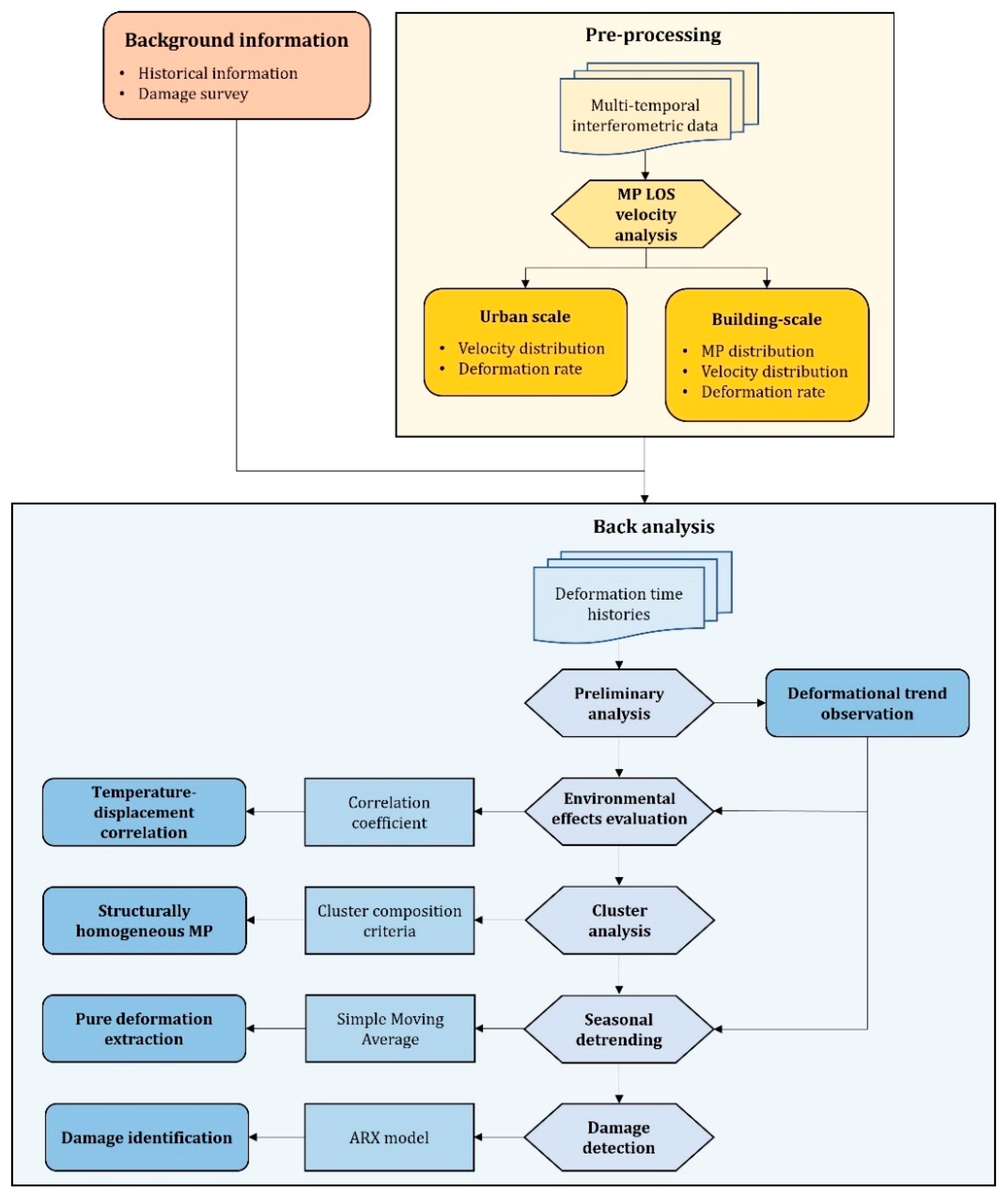
2.2.1. Background Information

The first part of the analysis begins by collecting principal information about the building itself, taking into account different aspects of its structural features and conditions: the literature review on the historical background of the structure, mainly addressed to define the constructive development of the building and its principal features, as well as the analysis of geometry and other surveys, in order to collect information on the conservation state or potential criticalities, have to be carefully developed. Thus, the most important general aspects of Palazzo Primoli are investigated to achieve an overall global knowledge of the building. The analysis includes:

• a brief history of Palazzo Primoli and its major constructive phases;
• geometric survey and drawings;
• critical evaluation of the building, including damage and crack patterns.

2.2.2. Pre-Processing

Multi-interferometric data analysis starts within the Pre-processing section. In this section, primary analysis of satellite data is performed by evaluating mean LOS displacement velocity (V_LOS), for initial detection of displacements around Palazzo Primoli. The study is subdivided into two parts, depending on the scale of analysis: urban and single-building scale. Urban scale analysis considers the whole satellite data and aims at highlighting areas characterized by the highest deformation rate inside the city. A brief statistical analysis is accomplished to recognize the distribution of V_LOS values in the entire data. For a better comprehension of deformations, the pointwise distribution is transformed into a continuous map through a spatial interpolation approach, the Inverse-Distance-Weighting (IDW) technique [49]: this method has been widely employed in the field of interferometric analysis to interpolate different parameters of satellite data [50,51,52,53,54]. Interpolation is carried out through quadratic weighting and by defining the AOI (Area Of Interest) inside a Geographical Information System (GIS) environment, such as QGIS [55], for both orbits. Interpolated maps are then used to estimate real displacement components, computed from a combination of ascending and descending data on pixels common to both maps. Vertical and east-west deformations are calculated through the expressions:

$${\mathrm{V}}_{\mathrm{vertical}}=\frac{{(\mathrm{V}}_{\mathrm{LOS},\mathrm{desc}}/{\mathrm{e}}_{\mathrm{desc}})-{(\mathrm{V}}_{\mathrm{LOS},\mathrm{asc}}/{\mathrm{e}}_{\mathrm{asc}})}{{(\mathrm{h}}_{\mathrm{desc}}/{\mathrm{e}}_{\mathrm{desc}})-{(\mathrm{h}}_{\mathrm{asc}}/{\mathrm{e}}_{\mathrm{asc}})}$$

(1)

$${\mathrm{V}}_{\mathrm{horizontal}}=\frac{{(\mathrm{V}}_{\mathrm{LOS},\mathrm{desc}}/{\mathrm{h}}_{\mathrm{desc}})-{(\mathrm{V}}_{\mathrm{LOS},\mathrm{asc}}/{\mathrm{h}}_{\mathrm{asc}})}{{(\mathrm{e}}_{\mathrm{desc}}/{\mathrm{h}}_{\mathrm{desc}})-{(\mathrm{e}}_{\mathrm{asc}}/{\mathrm{h}}_{\mathrm{asc}})}$$

(2)

where V_LOS,desc, and V_LOS,asc are the mean LOS displacement velocity, respectively, for descending and ascending orbits, while h and e are horizontal and vertical directional cosines of the respective orbit [50].

Single-building scale analysis aims to define a primary evaluation of the displacement rate of Palazzo Primoli. After geographical referencing of MPs on QGIS and Google Earth Pro [56], the study starts examining the points distribution both from a planimetric and an elevation point of view. Moreover, MPs are classified in relation to V_LOS values to interpret the global displacement rate on the structure. For the same purpose, real deformation components are now qualitatively detected through the use of single data: vertical and horizontal displacements are calculated by dividing ascending and descending LOS velocity values respectively by vertical and horizontal directional cosines, modifying the expressions defined in [57], as:

$${\mathrm{V}}_{\mathrm{vertical},\mathrm{asc}}=\frac{{\mathrm{V}}_{\mathrm{LOS},\mathrm{asc}}}{{\mathrm{h}}_{\mathrm{asc}}},{\mathrm{V}}_{\mathrm{vertical},\mathrm{desc}}=\frac{{\mathrm{V}}_{\mathrm{LOS},\mathrm{desc}}}{{\mathrm{h}}_{\mathrm{desc}}}$$

(3)

$${\mathrm{V}}_{\mathrm{horizontal},\mathrm{asc}}=\frac{{\mathrm{V}}_{\mathrm{LOS},\mathrm{asc}}}{{\mathrm{e}}_{\mathrm{asc}}},{\mathrm{V}}_{\mathrm{horizontal},\mathrm{desc}}=\frac{{\mathrm{V}}_{\mathrm{LOS},\mathrm{desc}}}{{\mathrm{e}}_{\mathrm{desc}}}$$

(4)

where V_vertical,asc, and V_{horizontal,asc} are vertical and horizontal components retrieved from ascending data, while V_{vertical,desc}, and V_{horizontal,desc} derive from descending one.

2.2.3. Back Analysis

The main body of the proposed methodology focuses on the back analysis of the building and analyzes displacement time histories of detected measurement points. A preliminary analysis of time histories is performed to understand global displacements/rotations of the structure, provide initial information, and, mostly, observe the presence of deformational trends which may affect displacement series. At first, displacement time series have been singularly analyzed; then, they were subdivided and examined into elevation groups, based on their altitude from the ground and referred to the examined structure, i.e., the structural element they refer to; last, mean displacement time series are calculated for the three detected elevation groups (ground floor, second floor, and rooftop) for both ascending and descending data. After the time series analysis, the correlation between environmental effects and recorded displacements is performed to evaluate the influence of external parameters on measured displacements [58,59]. Firstly, displacement time series are resampled weekly to fill gaps within various time windows; later, for each date, a measure of average daily temperature is retrieved from Roma Urbe meteorological station [60]. Thus, the correlation between temperature and displacement analysis is evaluated through the Pearson coefficient [61], as for the expression:

$${\mathrm{r}}_{\mathrm{td}}=\frac{\mathrm{cov}(\mathrm{t},\mathrm{d})}{{\mathsf{\sigma }}_{\mathrm{t}}{\mathsf{\sigma }}_{\mathrm{d}}}$$

(5)

where t and d are temperatures and resampled displacement time series of a single MP, and σ_t and σ_d are the standard deviation of the two parameters [62,63].

Later, the whole analysis focuses on the most vulnerable parts of the structure, defined according to both the Pre-processing analysis and the crack pattern of the building. In the case of Palazzo Primoli, the study examines in depth the balconies of the second and third floors of the building and a portion of the rooftop that is strictly linked with the balconies. Cluster analysis is performed to locate structurally homogeneous MPs within the three areas mentioned above. Different clustering criteria are chosen to highlight similarities and differences between the selected MPs. The criteria are:

• qualitative analysis of displacement time series: observation of time series and their relationship aims to identify a similar deformation evolution.
• quantitative comparison of displacement time series through two correlation coefficients, such as:

  a.

  Pearson correlation coefficient r_xy:

  $${\mathrm{r}}_{\mathrm{xy}}=\frac{\mathrm{cov}(\mathrm{x},\mathrm{y})}{{\mathsf{\sigma }}_{\mathrm{x}}{\mathsf{\sigma }}_{\mathrm{y}}}$$

  (6)

  where x and y are the displacement time series of two MPs, and σ_x and σ_y are the standard deviation of the series [62,63];

  b.

  deviation B between MPs time series:

  $$\mathrm{B}={\displaystyle \sum }_{\mathrm{i}=1}^{\mathrm{M}}{{(\mathrm{x}}_{\mathrm{i}} {-\mathrm{y}}_{\mathrm{i}})}^2$$

  (7)

  where x and y are the displacement time series of two MPs and M is the number of dates [36];

• proximity analysis of MPs: evaluation of planimetric and elevation location of each MP. Every MP inside a cluster must be within:
  • a 2 m radius neighborhood from the center in planimetry of the cluster.
  • a 2 m radius neighborhood from the center in elevation of the cluster.

After highlighting the interdependence between temperature and deformation, a seasonal detrending technique is applied to remove the environmental component from displacement time series and detect irreversible and pure deformation. For this purpose, the simple moving average (SMA) method [64] is implemented following the expression:

$${\mathrm{SMA}}_{\mathrm{m}}=\frac{{\mathrm{P}}_{\mathrm{m}}{+\mathrm{P}}_{\mathrm{m}-1}+\cdots {+\mathrm{P}}_{\mathrm{m}-(\mathrm{n}-1)}}{\mathrm{n}}$$

(8)

where P_m is the displacement value at instant m and n is the number of values included inside the mean calculation [65,66]. In this case, an annual moving average is performed by applying n = 52 moving dates to obtain the displacement at instant m, which is determined by averaging an entire year of previous values to consider environmental and noise effects. The AutoRegressive output with an eXogenous input part model (ARX) is then employed for deeper analysis of trends recognition inside time series, but also to develop an automated damage detection system. This technique belongs to black-box methods, as it is a system identification model aiming at defining the output of a signal from the initial input without any interest in the internal function of the signal itself [67]. Considering a Single Input—Single Output model (SISO), the ARX model follows the expression:

$${\mathrm{y}}_{\mathrm{k}}{+\mathrm{a}}_1{\mathrm{y}}_{\mathrm{k}-1}+\cdots {+\mathrm{a}}_{{\mathrm{n}}_{\mathrm{a}}}{\mathrm{y}}_{\mathrm{k}-{\mathrm{n}}_{\mathrm{a}}}={\mathrm{b}}_1{\mathrm{u}}_{\mathrm{k}}{+\mathrm{b}}_2{\mathrm{u}}_{\mathrm{k}-{\mathrm{n}}_{\mathrm{k}}-1}+\cdots {+\mathrm{b}}_{{\mathrm{n}}_{\mathrm{b}}}{\mathrm{u}}_{\mathrm{k}-{\mathrm{n}}_{\mathrm{k}}-{\mathrm{n}}_{\mathrm{b}}+1}{+\mathrm{e}}_{\mathrm{k}}$$

(9)

where y_k represents the final output of the model at instant k and u_k is the input parameter; terms a_i (i = 1, …, n_a) and b_i (i = 1, …, n_b) are, respectively, the regression coefficients of the autoregressive part, with a n_a order, and the exogenous part, with an n_b order; n_k is the delay order, representing potential delay between input and output signals; e_k is the residual error of the regression [59,68,69,70,71,72,73].

Table 3. ARX model implementing—ascending data.

Phase	Period	Samples Number	Data	Data Type
Estimation phase	21 March 2011– 29 December 2013	146	Input	Temperature
			Output	LOS displacements
Validation phase	5 January 2014– 17 March 2019	272	Input	Temperature
			Output	LOS displacements

summarizes the information for ARX model implementation.

The whole procedure is implemented in a Matlab algorithm through the system identification toolbox [74]. Initially, estimation and validation phases are defined: for the estimation period, a more than two-year-long term is chosen to permit the model to perform a better calibration of seasonal deformation cycles; the validation period lasts the remaining years. During the estimation phase, the model is built using the temperature dataset as input and LOS displacement as output. This process identifies an ideal displacement time series, which is then tested in the validation phase introducing the remaining part of the temperature data. Thus, uploading LOS displacement data of the validation period, residuals e_k between the ideal model and real measured parameter are calculated and, starting from them, three coefficients are derived for the evaluation of the quality of the model:

• The goodness of fit (GOF) [75], evaluated by means of the absolute error index of the Normalized Root Mean Squared Error (NRMSE):

$$\mathrm{GOF}=\left(1-\mathrm{NRMSE}\right)\%=\left(1-\frac{\sqrt{\frac{{{\displaystyle \sum }}_{\mathrm{k}=1}^{\mathrm{N}}{\mathrm{e}}_{\mathrm{k}}^2}{\mathrm{N}}}}{\overline{\mathrm{y}}}\right)\%$$

(10)

2.

Loss function λ₀ [76]:

$${\mathsf{\lambda }}_0=\frac{1}{\mathrm{N}}\sqrt{{\displaystyle \sum }_{\mathrm{k}=1}^{\mathrm{N}}{\mathrm{e}}_{\mathrm{k}}^2}$$

(11)

3.

Final prediction error (FPE) [77]:

$${\mathrm{FPE}=\mathsf{\lambda }}_0\frac{1+\frac{\mathrm{d}}{\mathrm{N}}}{1-\frac{\mathrm{d}}{\mathrm{N}}}.$$

(12)

Among all possible combinations between [n_a, n_b, n_k ] = [1:10, 1:10, 1:10], the best fitting ARX model was selected considering the highest GOF, the lowest λ₀, and the lowest FPE: comparing the model and the real data, the first parameter evaluates the accuracy of the fitting while the others define the misfitting level. For detection of possible outliers, a confidence interval of 95% was set, with a range of:

$$[\mathrm{y}-{\mathrm{t}}_{\mathsf{\alpha }/2,\mathsf{\nu }}{\mathsf{\sigma }}_{\mathrm{y}}{;\mathrm{y}+\mathrm{t}}_{\mathsf{\alpha }/2,\mathsf{\nu }}{\mathsf{\sigma }}_{\mathrm{y}}]$$

(13)

where y is the output value in the estimation phase, t represents the Student’s T distribution of parameter y and σ_y is its standard deviation. Thus, if residuals remain inside the confidence interval, the structural condition is stable; conversely, if residuals exceed the confidence interval, an instability phenomenon may have occurred.

2.3. The Case Study Application: Palazzo Primoli, Rome

Palazzo Primoli is a historical building in the center of Rome, not far from the main landmarks of the city (such as Castel Sant’Angelo, Pantheon, and Vatican City) (Figure 2a).

The palace stretches alongside Giuseppe Zanardelli street, within the I Municipio of the city, and it lies near the banks of the Tiber river. Nowadays, the city municipality, alongside the Primoli Foundation, owns Palazzo Primoli, which is the location of the Napoleonic Museum, the Mario Praz Museum, and the Primoli Foundation itself.

3. Results

3.1. Background Information

The palace was erected at the beginning of the XVI century for the Gottifredi family and was subsequently bought by count Luigi di Gioacchino Primoli in 1828. The current layout of Palazzo Primoli only partially derives from the original plan, since the building was deeply modified between 1904 and 1911, due to changes in the roads which run north and west of the palace [78,79]. Because of the presence of significant crack patterns on the eastern part of the structure, on-site inspections were held at the request of the managing bodies, who supplied previous geometric and critical surveys. Figure 3a shows cracks in different structural elements in the rooms on the ground and first floor (Figure 3b). The whole crack pattern is mainly located in rooms under the second-floor balcony, where another crack runs longitudinally to the balcony. However, the damage pattern could not be monitored since an on-site monitoring system has never been installed on Palazzo Primoli. Moreover, the cracks have not been correlated to any evident cause, as no heavy restoration works have occurred on the structure, nor damaging events have been registered in the surroundings.

3.2. Pre-Processing

The MPs classification based on the annual LOS displacement velocity of the whole data is presented in

Table 4. Mean LOS displacement velocity distribution of the whole data.

Orbit	VLOS [cm/Year]
	VLOS ≥ 0.00	VLOS < 0.00
Ascending MPs	18.2%	81.8%
Descending MPs	31.0%	69.0%

and

Table 5. Mean LOS displacement velocity distribution of the whole data in the interval of relative stability.

Orbit	VLOS [cm/Year]
	VLOS > +0.15	+0.15 ≥ VLOS ≥ −0.15	VLOS < −0.15
Ascending MPs	0.3%	93.0%	6.7%
Descending MPs	0.5%	95.3%	4.2%

. Most MPs assume negative values along the LOS both in ascending and descending orbits, which gives the idea of a global vertical motion of the analyzed area: negative values indicate movement away from the satellite along the LOS direction, while positive ones refer to movements towards the satellite. The LOS velocity distribution, then, does not appear to be dangerous as most of the values remain inside the so-called “interval of relative stability”, a threshold of LOS velocity values commonly fixed at V_LOS = ±0.15 cm/year [80]. However, some points reach higher negative values, confirming the deformation trend away from the satellite.

Figure 4 presents the distribution of processed MPs in the city center of Rome, which are distinguished based on their LOS velocity value. The maps highlight corresponding results between ascending and descending data, with comparable areas characterized by similar velocity measures, as demonstrated by the sector on the left bank of the Tiber, where the upper sector detects positive values for both orbits, while the lower neighboring part shows negative values.

Figure 5 displays the spatial distribution of LOS velocity values, defined through the IDW spatial interpolation algorithm applied to both ascending and descending data, using a pixel width of 8 × 11 m. Some areas subjected to deformation can be detected by observing the contour maps of the V_LOS parameter: a wide area with positive values is recognized in the western part of the city center; the rest of the map exhibits slightly negative values, which become more severe on the right and left banks of the lower part of Tiber River.

Figure 6 shows vertical and horizontal E-W displacements, computed by combining the two satellite orbits using Equations (1) and (2). The maps report a generally stable situation regarding horizontal deformation of the area and a more variable condition for vertical displacements, which approximately display a distribution similar to LOS velocity. However, the area surrounding the case study (highlighted with a red circle) presents a relatively stable condition. Moreover, the displayed results are consistent with previous satellite investigations held in the city center of Rome, such as [1], performed by processing ERS-1/2 and ENVISAT images spanning from 1992 to 2020 through SBAS-DInSAR, and [39], where CSK datasets from 2011 to 2013 are processed through the PSInSAR method.

Focusing on the case study, its relative MPs are retrieved from the whole data through a geographical selection. The points are then analyzed and firstly subdivided into three main elevation categories (ground floor, second floor, and rooftop) based on their altitude:

Table 6. Palazzo Primoli’s MPs classification based on their elevation.

Orbit	G (Ground Floor)	S (Second Floor)	R (Rooftop)
Ascending MPs	18%	24%	58%
Descending MPs	9%	48%	43%

provides the subdivision of points.

The points are then analyzed referring to their LOS velocity, as presented in

Table 7. Mean LOS displacement velocity distribution for Palazzo Primoli.

Orbit	VLOS [cm/Year]
	VLOS ≥ 0.00	VLOS < 0.00
Ascending MPs	8.7%	91.3%
Descending MPs	2.2%	97.8%

and

Table 8. Mean LOS displacement velocity distribution in the interval of relative stability for Palazzo Primoli.

Orbit	VLOS [cm/Year]
	VLOS > +0.15	+0.15 ≥ VLOS ≥ −0.15	VLOS < −0.15
Ascending MPs	0.5%	96.0%	3.5%
Descending MPs	0.5%	93.5%	6.0%

, and displayed in Figure 7. The results point out a significant prevalence of negative values both for the ascending and descending orbit, scattered on the whole structure: this outcome remarks the idea of a potential slight tendency to downward movements of the entire building. However, almost all MPs are characterized by very low LOS velocity values, remaining inside the above-mentioned “interval of relative stability”.

Once the LOS velocity distribution is defined, vertical and horizontal deformation rates are analyzed by means of Equations (3) and (4). Results are presented in Figure 8: horizontal displacements are not significative, as ascending and descending data provide opposite components since their MPs have similar LOS velocity values but discordant horizontal directional cosine; conversely, the presence of vertical deformations, even though with a relatively low intensity of 0.00 cm/year ≤ V_U ≤ +0.20 cm/year, is confirmed, as there is correspondence between results from both orbits.

3.3. Back Analysis

The back analysis starts by examining the deformation time series for each point identified for Palazzo Primoli. Figure 9 represents the mean displacement time series for each above-mentioned elevation category, both in ascending and descending orbits (March 2011–March 2019 for ascending orbit; July 2011–March 2019 for descending orbit). Each curve displays negative LOS displacements during the whole monitoring period for all three groups of MPs.

Moreover, time series provide deeper information regarding the development of deformations. The evolution of displacements can be subdivided into three main periods: a first one, with stable and periodic deformations; then, a phase characterized by more severe displacements, from the end of 2014 to the second half of 2015; finally, another interval with periodic deformations.

The analysis suggests that the occurred deformations may not have been constant during the whole monitoring period, but they could have developed during a specific term. Moreover, seasonal displacement trends can be observed, as time series show periodic variations that may depend on environmental effects, such as temperature.

The correlation between displacements and temperature is deeper analyzed through Pearson correlation coefficient r_td, as described in (5), and results are displayed in Figure 10a. Despite the initial idea, the distribution of r_td shows a very low correlation between the examined parameters. Further analyses are performed considering two distinct periods, and excluding the previously highlighted central part characterized by significant displacements.

When the same Pearson correlation coefficient is applied, results provide higher correlation values, as presented in Figure 10b,c: for example, considering values greater than r_td ≥ 0.4, the analysis defines an average correlation growth of 19% and 35%, respectively, for the ascending and descending data.

Subsequently, the analysis focuses on the second-floor balcony, the third-floor balcony, and a related portion of the rooftop of Palazzo Primoli since these areas are considered more vulnerable due to the observed damage pattern.

Cluster analysis of structurally homogeneous points is performed to highlight MPs with similar deformational behavior, following the criteria described in Section 2.2.3. A spatial proximity criterion was employed to overcome the low accuracy in the elevation position of the MPs in Palazzo Primoli, which is caused by MT-InSAR positioning inaccuracies (e.g., for MT-InSAR processing with CSK acquisitions, the positioning error is about 1–3 m [81]). Figure 11 shows the identified clusters based on the area they belong to. Because of the lack of points, not all sectors are equally represented by clusters: ascending data provides clusters on the central part of the investigated areas, while external parts are not covered at all; on the other hand, the descending orbit detects homogenous clusters in peripheral parts. It is worth mentioning that only one cluster is identified on the second-floor balcony: this aspect represents a great limit and influences the whole analysis, as that balcony is where the damage occurred.

Results from ascending clusters will only be presented in this work, as they are in the most vulnerable areas according to the observed crack pattern. The mean LOS velocity time series of all recognized clusters are presented in Figure 12a,c,e. Through the simple moving average method (Equation (8)), the same time series are filtered from seasonal environmental effects to define pure residual deformation trends. In Figure 12b,d,f, the corresponding SMA series are displayed from January 2013 to March 2019. Deformation curves confirm the previous interpretation of the LOS time series: displacements occurred in the central part of the monitoring period in all three analyzed areas; the deformation rate is not constant as clusters identify slightly different values; starting from the end of 2014 and the beginning of 2015, displacements tend to decrease, when conditions of relative stability appear inside all SMA series.

Last, the ARX model is applied to the above-mentioned clusters.

Table 9. ARX model results—ascending clusters.

Cluster	na	nb	nk	λ0	FPE	Goodness of Fit
s1	10	10	4	0.0004	0.0004	76.5%
t1	10	10	2	0.0007	0.0011	80.3%
t4	10	10	4	0.0004	0.0006	82.8%
c1	10	10	8	0.0002	0.0004	76.3%
c4	10	10	4	0.0006	0.0009	81.3%

presents values of initial processing and evaluation of the regressive model for each of the analyzed clusters. Results from all three parameters prove high consistency in fitting LOS time series with the ARX model, as the comparison between real displacements and model output detects low values of λ₀ and FPE, as well as high measures of GOF (with values higher than 75%), for the examined clusters.

The most outstanding cases are presented as an example. After evaluating the regressive parameters for each cluster, ideal curves defined by the ARX model (blue curve) are compared with the corresponding mean LOS displacement time series (red curve), as displayed in Figure 13a,c,e,g,i.

The comparison between ARX model outputs and LOS displacement time series recalls the previous interpretation of time series: while the estimation phase presents similar behaviors on both curves for the majority of clusters, in the following validation phase a different trend is visible, with LOS displacement curves shifting towards more intense values in the negative direction. Residuals are then computed as the difference between real and estimated displacements, as shown in Figure 13b,d,f,h,j, and they confirm the earlier hypothesis of structural behavior: the curves show a first period that is relatively stable, which is followed by an increment of negative displacements. The damage identification process is retrieved from evaluating a confidence interval, displayed in Figure 13b,d,f,h,j, stated at 95%, defining α = 0.05 in (13). The system provides meaningful results for the stability assessment of Palazzo Primoli, as many of the analyzed clusters show displacements that come out of the confidence interval, indicating irreversible deformation trends. Moreover, residual curves of clusters (except for t1) show a good correspondence in detecting the beginning of damaging displacements, as they all overcame the confidence interval during the second half of 2014 or the beginning of 2015, further confirming the results of the assessment.

4. Discussion

Considering the whole process, the present study has pointed out some issues in the interferometric analysis. The first topic concerns the georeferencing quality of data produced by MT-InSAR methods. During the analysis, a significant deficiency in the precision of MPs positioning has been experienced, especially in the elevation parameter. Clear errors were identified in the altitude of points, whereas the planimetric geolocation may be considered sufficiently accurate. Comparing the actual height of Palazzo Primoli, it is evident an overestimation in the elevation parameter. This issue in the georeferencing could also lead to a misinterpretation of data since analyzed MPs could refer both to structural and non-structural elements (e.g., tiles, railings, chimneys), where the deformational trend of the latter does not necessarily coincide with the global structural behavior. Further research needs to be developed, both to decrease such georeferencing errors, and to consider potential errors in geocoding caused by representation and GIS software.

In addition, the entire work points out a strong contrast between information brought by V_LOS values, which are defined on the whole monitoring period, and accurate analysis of LOS displacement time series for each MP. Indeed, results displayed from the first parameter seem to provide a relatively stable condition, as most points present low values of annual LOS displacement, remaining inside the stability thresholds: this trend is also confirmed by previous studies on the area of Rome, where similar displacement rates have been highlighted; conversely, the further analysis of deformation time series gives a more critical view of the displacement rate, identifying and confirming, by means of the damage detection system, a trend of deterioration. Such analysis highlights that it is not reliable to use only the V_LOS parameter as an index for assessing building stability, but a more accurate investigation of time series should be performed to determine the displacement rate of a structure. Further inspections and data from the on-site monitoring system would be a suitable tool for both assessing stability and validating interferometric results. In the case of Palazzo Primoli, the presence of displacement transducers on the structure on major cracks could have represented a potential source of information for both validating the displayed results and determining with higher accuracy the structural behavior of Palazzo Primoli, in particular for the balconies and the rooftop.

Combining satellite and in-situ monitoring has now gathered increasing interest in the field of SHM since the results from both methods can lead to widening resources for predicting structural damages and preserving both strategic structures and cultural heritage monuments.

Lastly, results given by the Pearson coefficient on correlation analysis between LOS displacements and temperature are heavily influenced by two aspects. First, the noisiness of satellite MPs time series can affect the comparison between parameters, as their high standard deviation decreases the correlation coefficient. Moreover, as previously stated, the analyzed MPs can be referred to as non-structural elements, whose deformational behavior could not necessarily depend on any environmental parameters.

5. Conclusions

In recent years, Satellite MT-InSAR methods have proven successful efficacy for remotely monitoring civil structures and infrastructures involved in damaging phenomena such as local or global deformations and rotations. The interferometric technique represents a powerful support for traditional SHM systems, as satellite monitoring enables the free, non-invasive, and widespread collection of displacement data on structures inside large areas. Moreover, MT-InSAR methods allow the performance of back analyses of past deformation, providing an effective tool for detecting structural vulnerabilities and damage. This work presents a methodology for interpreting and analyzing interferometric satellite data, aiming at providing a guideline to facilitate the use of this new technique.

The protocol splits into three main sections (Background information, Pre-processing, and Back analysis), characterized by specific tasks and methods: at first, the gathering of background information on the examined structure; later, analyzing LOS velocity values at urban and building scales; last, testing time series for detrending and damage detection. In addition, the protocol considers two different perspectives of analysis, at both urban and single-building scales. Thus, the methodology seeks to achieve the detection of displacements by taking advantage of the different capabilities and potentialities of satellite monitoring. The whole analysis consists of examining mean annual LOS displacement velocity and displacement time series. Moreover, data are processed through different techniques (IDW for spatial interpolation, Pearson correlation analysis, cluster analysis, SMA, and ARX regression for detrending and time series analysis) to optimize interferometric information and to allow detecting displacements during various levels of analysis. Throughout the whole analysis, algorithms derived from traditional on-site monitoring are applied to interferometric data.

Two data (ascending and descending) deriving from the SBAS-DInSAR processing of CSK images, dating back from 2011 to 2019, were employed to validate the proposed methodology on a specific building: Palazzo Primoli, a XVI-century building in the historical center of Rome. The achieved outcome demonstrated the effectiveness of the methodology. At first, the territorial scale deformation of Palazzo Primoli’s surroundings, and the center of Rome, was defined through mean annual LOS displacement velocity. The results showed consistency with previous studies on the city of Rome held. Later, the global deformation of Palazzo Primoli was recognized, stating a potential slight vertical movement of the structure, that comes along with the urban scale analysis. Last, a diagnosis of structural damage was hypothesized through inspection of local displacement time series: applying clustering, detrending, and regression techniques the presence, temporal evolution, and intensity of past deformations were detected in three vulnerable areas. Thus, the application of satellite interferometric data for SHM purposes has exhibited its potential contribution to assessing the condition and behavior of structures.

Among the different outcomes, the need for heavy post-processing of interferometric data, as well as deep and focused interpretation of results, were highlighted during the study and the design of the proposed methodology. The presented guideline still demands meticulous supervision and qualitative assessment, and further research for automatic processing must be analyzed. Unlike traditional on-site systems, that monitor specific parameters with high precision and reliability, satellite monitoring must be carefully read and interpreted and interferometric data must be properly processed to be connected to the actual damaged state of structures.

References

1. Zeni, G.; Bonano, M.; Casu, F.; Manunta, M.; Manzo, M.; Marsella, M.; Pepe, A.; Lanari, R. Long-Term Deformation Analysis of Historical Buildings through the Advanced SBAS-DInSAR Technique: The Case Study of the City of Rome, Italy. J. Geophys. Eng. 2011, 8, S1–S12. [Google Scholar] [CrossRef]
2. Ferretti, A.; Monti-Guarnieri, A.; Prati, C.; Rocca, F.; Massonet, D. InSAR Principles: Guidelines for SAR Interferometry: Processing and Interpretation; ESA TM; ESA publications: Noordwijk, The Netherlands, 2007; ISBN 978-92-9092-233-9. [Google Scholar]
3. Massonnet, D.; Feigl, K.L. Radar Interferometry and Its Application to Changes in the Earth’s Surface. Rev. Geophys. 1998, 36, 441–500. [Google Scholar] [CrossRef] [Green Version]
4. Rosen, P.A.; Hensley, S.; Joughin, I.R.; Li, F.K.; Madsen, S.N.; Rodriguez, E.; Goldstein, R.M. Synthetic Aperture Radar Interferometry. Proc. IEEE 2000, 88, 333–382. [Google Scholar] [CrossRef]
5. Chen, F.; Lasaponara, R.; Masini, N. An Overview of Satellite Synthetic Aperture Radar Remote Sensing in Archaeology: From Site Detection to Monitoring. J. Cult. Herit. 2017, 23, 5–11. [Google Scholar] [CrossRef]
6. Franceschetti, G.; Lanari, R. Synthetic Aperture Radar Processing; Electronic Engineering Systems Series; CRC Press: Boca Raton, FL, USA, 1999; ISBN 978-0-8493-7899-7. [Google Scholar]
7. Negula, I.D.; Sofronie, R.; Virsta, A.; Badea, A. Earth Observation for the World Cultural and Natural Heritage. Agric. Agric. Sci. Procedia 2015, 6, 438–445. [Google Scholar] [CrossRef] [Green Version]
8. Tapete, D.; Fanti, R.; Cecchi, R.; Petrangeli, P.; Casagli, N. Satellite Radar Interferometry for Monitoring and Early-Stage Warning of Structural Instability in Archaeological Sites. J. Geophys. Eng. 2012, 9, S10–S25. [Google Scholar] [CrossRef]
9. Tapete, D.; Cigna, F. Site-Specific Analysis of Deformation Patterns on Archaeological Heritage by Satellite Radar Interferometry. MRS Proc. 2012, 1374, 283–295. [Google Scholar] [CrossRef] [Green Version]
10. Luo, L.; Wang, X.; Guo, H.; Lasaponara, R.; Zong, X.; Masini, N.; Wang, G.; Shi, P.; Khatteli, H.; Chen, F.; et al. Airborne and Spaceborne Remote Sensing for Archaeological and Cultural Heritage Applications: A Review of the Century (1907–2017). Remote Sens. Environ. 2019, 232, 111280. [Google Scholar] [CrossRef]
11. Macchiarulo, V.; Giardina, G.; Milillo, P.; González Martí, J.; Sánchez, J.; DeJong, M.J. Settlement-Induced Building Damage Assessment Using MT-Insar Data for the Crossrail Case Study in London. In International Conference on Smart Infrastructure and Construction 2019 (ICSIC); ICE Publishing: Cambridge, UK, 2019; pp. 721–727. [Google Scholar]
12. Tang, P.; Chen, F.; Zhu, X.; Zhou, W. Monitoring Cultural Heritage Sites with Advanced Multi-Temporal InSAR Technique: The Case Study of the Summer Palace. Remote Sens. 2016, 8, 432. [Google Scholar] [CrossRef] [Green Version]
13. Zhou, W.; Chen, F.; Guo, H. Differential Radar Interferometry for Structural and Ground Deformation Monitoring: A New Tool for the Conservation and Sustainability of Cultural Heritage Sites. Sustainability 2015, 7, 1712–1729. [Google Scholar] [CrossRef] [Green Version]
14. Ferretti, A.; Prati, C.; Rocca, F. Permanent Scatterers in SAR Interferometry. IEEE Trans. Geosci. Remote Sens. 2001, 39, 8–20. [Google Scholar] [CrossRef]
15. Berardino, P.; Fornaro, G.; Lanari, R.; Sansosti, E. A New Algorithm for Surface Deformation Monitoring Based on Small Baseline Differential SAR Interferograms. IEEE Trans. Geosci. Remote Sens. 2002, 40, 2375–2383. [Google Scholar] [CrossRef] [Green Version]
16. Lanari, R.; Mora, O.; Manunta, M.; Mallorqui, J.J.; Berardino, P.; Sansosti, E. A Small-Baseline Approach for Investigating Deformations on Full-Resolution Differential SAR Interferograms. IEEE Trans. Geosci. Remote Sens. 2004, 42, 1377–1386. [Google Scholar] [CrossRef]
17. Agapiou, A.; Lysandrou, V. Detecting Displacements Within Archaeological Sites in Cyprus After a 5.6 Magnitude Scale Earthquake Event Through the Hybrid Pluggable Processing Pipeline (HyP3) Cloud-Based System and Sentinel-1 Interferometric Synthetic Aperture Radar (InSAR) Analysis. IEEE J. Sel. Top. Appl. Earth Obs. Remote Sens. 2020, 13, 6115–6123. [Google Scholar] [CrossRef]
18. Alani, A.M.; Tosti, F.; Ciampoli, L.B.; Gagliardi, V.; Benedetto, A. An Integrated Investigative Approach in Health Monitoring of Masonry Arch Bridges Using GPR and InSAR Technologies. NDT E Int. 2020, 115, 102288. [Google Scholar] [CrossRef]
19. Alberti, S.; Ferretti, A.; Leoni, G.; Margottini, C.; Spizzichino, D. Surface Deformation Data in the Archaeological Site of Petra from Medium-Resolution Satellite Radar Images and SqueeSARTM Algorithm. J. Cult. Herit. 2017, 25, 10–20. [Google Scholar] [CrossRef]
20. Aslan, G.; Cakir, Z.; Lasserre, C.; Renard, F. Investigating Subsidence in the Bursa Plain, Turkey, Using Ascending and Descending Sentinel-1 Satellite Data. Remote Sens. 2019, 11, 85. [Google Scholar] [CrossRef] [Green Version]
21. Cascini, L.; Ferlisi, S.; Fornaro, G.; Lanari, R.; Peduto, D.; Zeni, G. Subsidence Monitoring in Sarno Urban Area via Multi-temporal DInSAR Technique. Int. J. Remote Sens. 2006, 27, 1709–1716. [Google Scholar] [CrossRef]
22. Cavalagli, N.; Kita, A.; Falco, S.; Trillo, F.; Costantini, M.; Ubertini, F. Satellite Radar Interferometry and In-Situ Measurements for Static Monitoring of Historical Monuments: The Case of Gubbio, Italy. Remote Sens. Environ. 2019, 235, 111453. [Google Scholar] [CrossRef]
23. Cigna, F.; Del Ventisette, C.; Liguori, V.; Casagli, N. Advanced Radar-Interpretation of InSAR Time Series for Mapping and Characterization of Geological Processes. Nat. Hazards Earth Syst. Sci. 2011, 11, 865–881. [Google Scholar] [CrossRef]
24. Farneti, E.; Cavalagli, N.; Costantini, M.; Trillo, F.; Minati, F.; Venanzi, I.; Ubertini, F. A Method for Structural Monitoring of Multispan Bridges Using Satellite InSAR Data with Uncertainty Quantification and Its Pre-Collapse Application to the Albiano-Magra Bridge in Italy. Struct. Health Monit. 2023, 22, 353–371. [Google Scholar] [CrossRef]
25. Fiaschi, S.; Holohan, E.; Sheehy, M.; Floris, M. PS-InSAR Analysis of Sentinel-1 Data for Detecting Ground Motion in Temperate Oceanic Climate Zones: A Case Study in the Republic of Ireland. Remote Sens. 2019, 11, 348. [Google Scholar] [CrossRef] [Green Version]
26. Lasaponara, R.; Masini, N. Satellite Synthetic Aperture Radar in Archaeology and Cultural Landscape: An Overview: Editorial. Archaeol. Prospect. 2013, 20, 71–78. [Google Scholar] [CrossRef]
27. Luo, S.; Feng, G.; Xiong, Z.; Wang, H.; Zhao, Y.; Li, K.; Deng, K.; Wang, Y. An Improved Method for Automatic Identification and Assessment of Potential Geohazards Based on MT-InSAR Measurements. Remote Sens. 2021, 13, 3490. [Google Scholar] [CrossRef]
28. Macchiarulo, V.; Milillo, P.; Blenkinsopp, C.; Giardina, G. Monitoring Deformations of Infrastructure Networks: A Fully Automated GIS Integration and Analysis of InSAR Time-Series. Struct. Health Monit. 2022, 21, 1849–1878. [Google Scholar] [CrossRef]
29. Moise, C.; Dana Negula, I.; Mihalache, C.E.; Lazar, A.M.; Dedulescu, A.L.; Rustoiu, G.T.; Inel, I.C.; Badea, A. Remote Sensing for Cultural Heritage Assessment and Monitoring: The Case Study of Alba Iulia. Sustainability 2021, 13, 1406. [Google Scholar] [CrossRef]
30. Necula, N.; Niculiță, M.; Fiaschi, S.; Genevois, R.; Riccardi, P.; Floris, M. Assessing Urban Landslide Dynamics through Multi-Temporal InSAR Techniques and Slope Numerical Modeling. Remote Sens. 2021, 13, 3862. [Google Scholar] [CrossRef]
31. Pepe, A.; Sansosti, E.; Berardino, P.; Lanari, R. On the Generation of ERS/ENVISAT DInSAR Time-Series Via the SBAS Technique. IEEE Geosci. Remote Sens. Lett. 2005, 2, 265–269. [Google Scholar] [CrossRef]
32. Selvakumaran, S.; Plank, S.; Geiß, C.; Rossi, C.; Middleton, C. Remote Monitoring to Predict Bridge Scour Failure Using Interferometric Synthetic Aperture Radar (InSAR) Stacking Techniques. Int. J. Appl. Earth Obs. Geoinf. 2018, 73, 463–470. [Google Scholar] [CrossRef]
33. Urrego, L.E.B.; Verstrynge, E.; Balen, K.V.; Wuyts, V.; Declercq, P.-Y. Settlement-Induced Damage Monitoring of a Historical Building Located in a Coal Mining Area Using PS-InSAR. In 6th Workshop on Civil Structural Health Monitoring; Queen’s University: Belfast, UK, 2016; pp. 1–8. [Google Scholar]
34. Xiong, S.; Wang, C.; Qin, X.; Zhang, B.; Li, Q. Time-Series Analysis on Persistent Scatter-Interferometric Synthetic Aperture Radar (PS-InSAR) Derived Displacements of the Hong Kong–Zhuhai–Macao Bridge (HZMB) from Sentinel-1A Observations. Remote Sens. 2021, 13, 546. [Google Scholar] [CrossRef]
35. Arangio, S.; Calò, F.; Di Mauro, M.; Bonano, M.; Marsella, M.; Manunta, M. An Application of the SBAS-DInSAR Technique for the Assessment of Structural Damage in the City of Rome. Struct. Infrastruct. Eng. 2014, 10, 1469–1483. [Google Scholar] [CrossRef]
36. Zhu, M.; Wan, X.; Fei, B.; Qiao, Z.; Ge, C.; Minati, F.; Vecchioli, F.; Li, J.; Costantini, M. Detection of Building and Infrastructure Instabilities by Automatic Spatiotemporal Analysis of Satellite SAR Interferometry Measurements. Remote Sens. 2018, 10, 1816. [Google Scholar] [CrossRef] [Green Version]
37. Ardizzone, F.; Bonano, M.; Giocoli, A.; Lanari, R.; Marsella, M.; Pepe, A.; Perrone, A.; Piscitelli, S.; Scifoni, S.; Scutti, M.; et al. Analysis of Ground Deformation Using SBAS-DInSAR Technique Applied to COSMO-SkyMed Images, the Test Case of Roma Urban Area. In Proceedings of the SPIE 8536, SAR Image Analysis, Modeling, and Techniques XII, Edinburgh, UK, 21 November 2011; Volume 85360D. [Google Scholar]
38. Bozzano, F.; Esposito, C.; Mazzanti, P.; Patti, M.; Scancella, S. Imaging Multi-Age Construction Settlement Behaviour by Advanced SAR Interferometry. Remote Sens. 2018, 10, 1137. [Google Scholar] [CrossRef] [Green Version]
39. Cigna, F.; Lasaponara, R.; Masini, N.; Milillo, P.; Tapete, D. Persistent Scatterer Interferometry Processing of COSMO-SkyMed StripMap HIMAGE Time Series to Depict Deformation of the Historic Centre of Rome, Italy. Remote Sens. 2014, 6, 12593–12618. [Google Scholar] [CrossRef] [Green Version]
40. Pepe, A.; Lanari, R. On the Extension of the Minimum Cost Flow Algorithm for Phase Unwrapping of Multitemporal Differential SAR Interferograms. IEEE Trans. Geosci. Remote Sens. 2006, 44, 2374–2383. [Google Scholar] [CrossRef]
41. Falabella, F.; Serio, C.; Masiello, G.; Zhao, Q.; Pepe, A. A Multigrid InSAR Technique for Joint Analyses at Single-Look and Multi-Look Scales. IEEE Geosci. Remote Sens. Lett. 2022, 19, 1–5. [Google Scholar] [CrossRef]
42. Ojha, C.; Manunta, M.; Lanari, R.; Pepe, A. The Constrained-Network Propagation (C-NetP) Technique to Improve SBAS-DInSAR Deformation Time Series Retrieval. IEEE J. Sel. Top. Appl. Earth Obs. Remote Sens. 2015, 8, 4910–4921. [Google Scholar] [CrossRef]
43. Bonano, M.; Manunta, M.; Marsella, M.; Lanari, R. Long-Term ERS/ENVISAT Deformation Time-Series Generation at Full Spatial Resolution via the Extended SBAS Technique. Int. J. Remote Sens. 2012, 33, 4756–4783. [Google Scholar] [CrossRef]
44. Di Carlo, F.; Miano, A.; Giannetti, I.; Mele, A.; Bonano, M.; Lanari, R.; Meda, A.; Prota, A. On the Integration of Multi-Temporal Synthetic Aperture Radar Interferometry Products and Historical Surveys Data for Buildings Structural Monitoring. J. Civ. Struct. Health Monit. 2021, 11, 1429–1447. [Google Scholar] [CrossRef]
45. Casu, F.; Manzo, M.; Lanari, R. A Quantitative Assessment of the SBAS Algorithm Performance for Surface Deformation Retrieval from DInSAR Data. Remote Sens. Environ. 2006, 102, 195–210. [Google Scholar] [CrossRef]
46. Bonano, M.; Manunta, M.; Pepe, A.; Paglia, L.; Lanari, R. From Previous C-Band to New X-Band SAR Systems: Assessment of the DInSAR Mapping Improvement for Deformation Time-Series Retrieval in Urban Areas. IEEE Trans. Geosci. Remote Sens. 2013, 51, 1973–1984. [Google Scholar] [CrossRef]
47. Talledo, D.A.; Miano, A.; Bonano, M.; Di Carlo, F.; Lanari, R.; Manunta, M.; Meda, A.; Mele, A.; Prota, A.; Saetta, A.; et al. Satellite Radar Interferometry: Potential and Limitations for Structural Assessment and Monitoring. J. Build. Eng. 2022, 46, 103756. [Google Scholar] [CrossRef]
48. Manunta, M.; De Luca, M.; Zinno, I.; Casu, F.; Manzo, M.; Bonano, M.; Fusco, A.; Pepe, A.; Onorato, G.; Berardino, P.; et al. The Parallel SBAS Approach for Sentinel-1 Interferometric Wide Swath Deformation Time-Series Generation: Algorithm Description and Products Quality Assessment. IEEE Trans. Geosci. Remote Sens. 2019, 57, 6259–6281. [Google Scholar] [CrossRef]
49. Shepard, D. A Two-Dimensional Interpolation Function for Irregularly-Spaced Data. In Proceedings of the 1968 23rd ACM National Conference; Association for Computing Machinery: New York, NY, USA, 1968; pp. 517–524. [Google Scholar]
50. Floris, M.; Fontana, A.; Tessari, G.; Mulè, M. Subsidence Zonation Through Satellite Interferometry in Coastal Plain Environments of NE Italy: A Possible Tool for Geological and Geomorphological Mapping in Urban Areas. Remote Sens. 2019, 11, 165. [Google Scholar] [CrossRef] [Green Version]
51. Lu, G.Y.; Wong, D.W. An Adaptive Inverse-Distance Weighting Spatial Interpolation Technique. Comput. Geosci. 2008, 34, 1044–1055. [Google Scholar] [CrossRef]
52. Matano, F.; Sacchi, M.; Vigliotti, M.; Ruberti, D. Subsidence Trends of Volturno River Coastal Plain (Northern Campania, Southern Italy) Inferred by SAR Interferometry Data. Geosciences 2018, 8, 8. [Google Scholar] [CrossRef] [Green Version]
53. Raspini, F.; Cigna, F.; Moretti, S. Multi-Temporal Mapping of Land Subsidence at Basin Scale Exploiting Persistent Scatterer Interferometry: Case Study of Gioia Tauro Plain (Italy). J. Maps 2012, 8, 514–524. [Google Scholar] [CrossRef] [Green Version]
54. Vilardo, G.; Ventura, G.; Terranova, C.; Matano, F.; Nardò, S. Ground Deformation Due to Tectonic, Hydrothermal, Gravity, Hydrogeological, and Anthropic Processes in the Campania Region (Southern Italy) from Permanent Scatterers Synthetic Aperture Radar Interferometry. Remote Sens. Environ. 2009, 113, 197–212. [Google Scholar] [CrossRef]
55. QGIS.org QGIS User Guide—QGIS Documentation. Available online: https://docs.qgis.org/3.22/en/docs/user_manual/index.html (accessed on 14 January 2022).
56. Google Earth User Guide Documentation. Available online: https://earth.google.com/intl/ar/userguide/v4/index.htm (accessed on 23 January 2022).
57. Di Traglia, F.; De Luca, C.; Manzo, M.; Nolesini, T.; Casagli, N.; Lanari, R.; Casu, F. Joint Exploitation of Space-Borne and Ground-Based Multitemporal InSAR Measurements for Volcano Monitoring: The Stromboli Volcano Case Study. Remote Sens. Environ. 2021, 260, 112441. [Google Scholar] [CrossRef]
58. Coccimiglio, S.; Coletta, G.; Lenticchia, E.; Miraglia, G.; Ceravolo, R. Combining Satellite Geophysical Data with Continuous On-Site Measurements for Monitoring the Dynamic Parameters of Civil Structures. Sci. Rep. 2022, 12, 2275. [Google Scholar] [CrossRef]
59. Lorenzoni, F.; Caldon, M.; da Porto, F.; Modena, C.; Aoki, T. Post-Earthquake Controls and Damage Detection through Structural Health Monitoring: Applications in l’Aquila. J. Civ. Struct. Health Monit. 2018, 8, 217–236. [Google Scholar] [CrossRef]
60. Clima Roma/Urbe—Dati Climatici. Available online: https://it.tutiempo.net/clima/ws-162350.html (accessed on 7 January 2022).
61. Lee Rodgers, J.; Nicewander, W.A. Thirteen Ways to Look at the Correlation Coefficient. Am. Stat. 1988, 42, 59–66. [Google Scholar] [CrossRef]
62. Hair, J.F.; Black, W.C.; Babin, B.J.; Anderson, R.E.; Tatham, R.L. Multivariate Data Analysis, 7th ed.; Pearson Education Limited: Harlow, UK, 2014; ISBN 978-1-292-02190-4. [Google Scholar]
63. Swinscow, T.D.V.; Campbell, M.J. Statistics at Square One, 10th ed.; BMJ: London, UK, 2002; ISBN 1-280-19790-0. [Google Scholar]
64. Johnston, F.R.; Boyland, J.E.; Meadows, M.; Shale, E. Some Properties of a Simple Moving Average When Applied to Forecasting a Time Series. J. Oper. Res. Soc. 1999, 50, 1267. [Google Scholar] [CrossRef]
65. Hansun, S. A Novel Research of New Moving Average Method in Time Series Analysis. Int. J. New Media Technol. IJNMT 2014, 1, 22. [Google Scholar]
66. Hyndman, R.J.; Athanasopoulos, G. Forecasting: Principles and Practice, 2nd ed.; OTexts: Heathmont, Australia, 2018; ISBN 978-0-9875071-1-2. [Google Scholar]
67. Ljung, L. System Identification: Theory for the User, 2nd ed.; Prentice-Hall Information and System Sciences Series; Prentice Hall PTR: Upper Saddle River, NJ, USA, 1999; ISBN 0-13-656695-2. [Google Scholar]
68. He, X. Vibration-Based Damage Identification and Health Monitoring of Civil Structures. Ph.D. Thesis, University of California San Diego, La Jolla, CA, USA, 2008. [Google Scholar]
69. Lorenzoni, F. Integrated Methodologies Based on Structural Health Monitoring for the Protection of Cultural Heritage Buildings. Ph.D. Thesis, Univerità degli Studi di Trento, Trento, Italy, 2013. [Google Scholar]
70. Peeters, B.; De Roeck, G. One Year Monitoring of The Z24-Bridge: Environmental Influences Versus Damage Events. Proc. SPIE Int. Soc. Opt. Eng. 2001, 30, 149–171. [Google Scholar]
71. Ramos, L. Damage Identification on Masonry Structures Based on Vibration Signatures. Ph.D. Thesis, University of Minho, Braga, Portugal, 2007. [Google Scholar]
72. Modena, C.; Lorenzoni, F.; Caldon, M.; da Porto, F. Structural Health Monitoring: A Tool for Managing Risks in Sub-Standard Conditions. J. Civ. Struct. Health Monit. 2016, 6, 365–375. [Google Scholar] [CrossRef]
73. Lorenzoni, F.; Casarin, F.; Caldon, M.; Islami, K.; Modena, C. Uncertainty Quantification in Structural Health Monitoring: Applications on Cultural Heritage Buildings. Mech. Syst. Signal Process. 2016, 66–67, 268–281. [Google Scholar] [CrossRef]
74. Ljung, L. System Identification ToolboxTM—User’s Guide; The Mathworks, Inc.: Natick, MA, USA, 2022. [Google Scholar]
75. Huber-Carol, C.; Balakrishnan, N.; Nikulin, M.S.; Mesbah, M. Goodness-of-Fit Tests and Model Validity; Birkhäuser: Boston, MA, USA, 2002; ISBN 978-1-4612-6613-6. [Google Scholar]
76. Wald, A. Statistical Decision Functions. Nature 1951, 167, 1044. [Google Scholar] [CrossRef]
77. Akaike, H. Fitting Autoregressive Models for Prediction. Ann. Inst. Stat. Math. 1969, 21, 243–247. [Google Scholar] [CrossRef]
78. Floridi, G. Il Palazzo Romano Filonardi Già Gottifredi, Poi Primoli in Piazza Dell’Orso. Strenna dei Romanisti 2004, LXV, 279–286. [Google Scholar]
79. Pietrangeli, C. Il Palazzo Primoli All’Orso. Strenna Dei Rom. 1965, XXVI, 341–344. [Google Scholar]
80. Tapete, D.; Cigna, F. Rapid Mapping and Deformation Analysis over Cultural Heritage and Rural Sites Based on Persistent Scatterer Interferometry. Int. J. Geophys. 2012, 2012, 618609. [Google Scholar] [CrossRef] [Green Version]
81. Wasowski, J.; Bovenga, F. Investigating Landslides and Unstable Slopes with Satellite Multi Temporal Interferometry: Current Issues and Future Perspectives. Eng. Geol. 2014, 174, 103–138. [Google Scholar] [CrossRef]
Figure 1. Flowchart of the proposed methodology.
Remotesensing 15 01177 g001
Figure 2. (a) Geographical context of Palazzo Primoli (highlighted inside the red circle) in the center of Rome; (b) top view of Palazzo Primoli.
Remotesensing 15 01177 g002
Figure 3. (a) Cross section of Palazzo Primoli and crack pattern; (b) crack on the first-floor ceiling.
Remotesensing 15 01177 g003
Figure 4. Mean LOS displacement velocity of MPs in the city center of Rome in the ascending (a) and descending orbit (b).
Remotesensing 15 01177 g004
Figure 5. Mean LOS displacement velocity interpolation on the city center of Rome in the ascending (a) and descending orbit (b).
Remotesensing 15 01177 g005
Figure 6. Mean vertical (a) and horizontal (b) displacement velocity interpolation on the city center of Rome.
Remotesensing 15 01177 g006
Figure 7. Mean LOS displacement velocity distribution on Palazzo Primoli in ascending (a) and descending (b) orbits.
Remotesensing 15 01177 g007
Figure 8. Mean displacement velocity distribution on Palazzo Primoli: vertical displacement in ascending (a), and descending (b) orbits; horizontal displacement in ascending (c), and descending (d) orbits.
Remotesensing 15 01177 g008aRemotesensing 15 01177 g008b
Figure 9. Mean LOS displacement time series of the three elevation categories in ascending (a), and descending (b) orbits. Vertical dotted lines define the interval of major displacement inside the whole monitoring period.
Remotesensing 15 01177 g009
Figure 10. Pearson correlation coefficient results in Palazzo Primoli MPs (a); Pearson correlation coefficient results in the first and second periods of time series for ascending (b), and descending (c) orbits.
Remotesensing 15 01177 g010
Figure 11. Cluster distribution on the three areas of Palazzo Primoli in ascending (a), and descending (b) orbits.
Remotesensing 15 01177 g011
Figure 12. Ascending clusters mean LOS time series in second (a), and third floor (c) balconies, and in the rooftop (e); ascending clusters SMA time series in second (b), and third floor (d) balconies, and in the rooftop (f). The curves for different clusters on the same floor are represented by a color scale consistent with the colors used in Figure 11 (blue for the second-floor balcony, green for the third-floor balcony, and yellow for the rooftop).
Remotesensing 15 01177 g012
Figure 13. ARX models output and residuals for damage identification on some clusters: cluster s1 (a,b), t1 (c,d), t4 (e,f), c1 (g,h), c4 (i,j).
Remotesensing 15 01177 g013aRemotesensing 15 01177 g013b