Abstract
The application of Transformer in computer vision has had the most significant influence of all the deep learning developments over the past five years. In addition to the exceptional performance of convolutional neural networks (CNN) in hyperspectral image (HSI) classification, Transformer has begun to be applied to HSI classification. However, for the time being, Transformer has not produced satisfactory results in HSI classification. Recently, in the field of image classification, the creators of Sequencer have proposed a Sequencer structure that substitutes the Transformer self-attention layer with a BiLSTM2D layer and achieves satisfactory results. As a result, this paper proposes a unique network called SquconvNet, that combines CNN with Sequencer block to improve hyperspectral classification. In this paper, we conducted rigorous HSI classification experiments on three relevant baseline datasets to evaluate the performance of the proposed method. The experimental results show that our proposed method has clear advantages in terms of classification accuracy and stability.
1. Introduction
Recent improvements in hyperspectral imaging sensors have resulted in hyperspectral images (HSI) that are rich in hundreds of contiguous and narrow spectral bands/depth. Due to its extensive spatial-spectral data, HSI has been used for a variety of purposes, including target detection [1], forestry [2,3], satellite calibration [4], identifying post-fire severity [5], and mineral identification [6]. Similarly, classification of hyperspectral land-cover information is one of the most significant application directions and has garnered a great deal of attention.
Two of the key distinguishing features of HSI are its high spatial correlation and an abundance of spectral information. A high spatial correlation from homogeneous areas can give secondary supplemental information for accurate mapping [7]. The ground material comprises a significant number of representative features that enable precise identification [8], taking advantage of the rich spectral information found in the continuous spectral bands. Contrarily, the curse of dimensionality is also brought on by an abundance of spectral information, which may have an impact on the performance of the classification [9,10,11]. Utilizing dimensionality reduction techniques is a crucial step for HSI classification, in order to improve the classification performance. The most used dimensionality reduction approach is Principal Component Analysis (PCA) [12]. In addition, other key dimensionality reduction techniques in hyperspectral classification include Factor Analysis (FA) [13], Linear Discriminant Analysis (LDA) [14,15], and Independent Discriminant Analysis (IDA) [16,17]. Early attempts at HSI classification included Support Vector Machines (SVMs) [18], Random Forest (RF) [19], K-mean clustering (KNN) [20], and Markov Random Field (MRF) [21]. However, because these techniques don’t concentrate on spatial correlation and local consistency, they struggle to fully utilize spatial feature information, which leads to subpar classification performance. Recent advances in deep learning-based techniques, such as deep neural networks, have had a major impact on computer vision and have also been introduced to HSI classification. A deep belief network (DBN) [22] and stacked autoencoders (SAE) [12] are two methods that call for flattening the input data patches into one-dimensional features. However, both techniques alter the original spatial data, which leads to subpar performances. Hu et al. suggested five convolutional layers to create a 1D-CNN [23] for HSI classification. It accepts spectral data as input and can successfully extract discriminative features from the spectral data. The data conveyed by the first few principal components after dimensionality reduction are used by a 2D-CNN method [24], to extract spatial features. Chen et al. [25], introduced 3D-CNN to HSI classification, in order to extract both spatial and spectral information. The spectral-spatial residual network (SSRN) [26], which was inspired by Resnet [27], creates a deeper structure and utilizes identity mapping to connect additional three-dimensional convolutional layers. The deep pyramidal residual network (DPRN) has also been proposed for HSI data [28]. According to [29], a hybrid-CNN model (HybridSN) is proposed, that may overcome the failure of 2D-CNN to extract discriminative features from the spectral dimension, and that scales back the complexity of a single 3D-CNN. In addition to the convolution neural network, various networks with exceptional performance have been introduced to HSI classification, such as the completely convolution network (FCN) [30,31], the generative adversarial network (GAN) [32,33], the graph convolutional network (GCN) [34], etc.
Additionally, Transformer, the most well-liked neural network currently, has been introduced into hyperspectral classification [35]. These include a Spatial-Spectral Transformer (SST) [36], an upgraded transformer (SAT) [37], a restructured transformer encoder with a cross-layer model (SpectralFormer) [38], and a Spectral-Spatial Feature Tokenization Transformer (SSFTT) [39]. However, the performance of these Transformer-based methods is inferior to that of CNN-based methods.
Transformer still has certain limitations regarding the extraction of local spectral and local information disparities, which causes performance bottlenecks. Convolutional neural networks perform well in HSI classification, although there are still a number of problems. The first is that the ground’s irregular shape prevents the convolution kernel from being able to capture all of its features [40]. The second is caused by the fact that the small convolutional kernels prevent convolutional neural networks’ receptive fields from matching the hyperspectral features across the whole bandwidth [37]. Recently, Yuki and Masato [41] proposed Sequencer, a unique and straightforward architecture that uses LSTM for image classification. Sequencer uses a BiLSTM2D layer to replace the multi-head attention layer in the transformer encoder to create Sequencer block. Experiments reveal that self-attention is not required for modeling remote dependencies, and that competitive performance can be attained using the LSTM instead. As a supplement to convolutional neural networks, we have developed Sequencer, a Sequencer made up of vertical and horizontal bidirectional LSTMs, based on the context of the aforementioned problems and inspired by Sequencer [41]. Similar to the convolutional layer, we take a pixel as the center, regard the vertical and horizontal directions as sequences, and simultaneously expand the pixel to form a spatially significant receptive field. Contrary to the convolutional layer, however, the timed information capacity of LSTM gives the Sequencer the ability to blend spatial information memory, which we feel can be employed as a supplement to the convolutional layer’s shortcomings. As a result, we suggest SquconvNet, a network integrating CNN with Sequencer2D block for HSI Classification, as being inspired by Sequencer. The proposed network in this study consists of three modules: the Spectral-Spatial Feature Extraction (SSFE) module, the Sequencer module, and the Auxiliary Classification (AC) module. The dimensionally reduced 3D-Patches input will be passed through the Sequencer module first, to capture long-term feature information, then the SSFE module will extract spatial features, and finally the AC module will further improve the classification performance. The LSTM shows a strong performance in utilizing long-range information to compensate for CNN’s shortcomings, and our proposed model has demonstrated good results on three standard datasets.
The following is a summary of this paper’s significant contributions and work:
- (1)
- We introduce the BiLSTM2D layer and Sequencer module for the first time, and combine them with CNN to compensate for CNN’s shortcomings and improve the performance of HSI classification.
- (2)
- A supplementary classification module comprised of two convolutional layers and a fully connected layer is proposed, with the dual purpose of decreasing the network parameters and assisting the network in classification.
- (3)
- Using three typical baseline datasets, we performed qualitative and quantitative evaluation studies (IP, UP, SA). The experimental findings show that, in terms of classification accuracy and stability, our proposed model verifies its superiority.
Next, Section 2 introduces in detail the illustration of the proposed SquconvNet architecture and its three modules. Section 3 describes the baseline datasets and presents an analysis of the experimental results. Ablation experiments and time loss are discussed in Section 4. Ultimately, the conclusion is drawn in Section 5.
2. Materials and Methods
2.1. Overview of SquconvNet
The proposed SquconvNet’s general structure is shown in Figure 1. It is composed of three modules: the Spectral-Spatial Feature Extraction Module, the Sequencer2D Module, and the Auxiliary Classification Module.
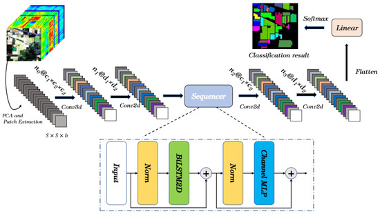
Figure 1.
Illustration of the proposed SquconvNet.
2.2. Spectral-Spatial Feature Extraction Module
The Spectral-Spatial Feature Extraction (SSFE) module is where the proposed SquconvNet starts. HybridSN [29] and SSFTT [39] served as the inspiration for the SSFE module’s design. Here, we adopt a comparable structure to them and improve its properties. The SSFE module primarily consists of a 3D-convolution layer and a 2D-convolution layer to reduce the amount of computation. Each convolution layer is followed by a batch normalization (BN) layer, a Relu non-linear activation, and another layer.
Firstly, an original HSI dataset is defined as , where D is the number of spectral bands, W is the width, and H is the height. Each HSI pixel forms a one-hot vector , where C is the classes of land-cover. However, since D bands make up the HSI data, they only add a lot of unnecessary calculations and non-useful information. To eliminate redundant spectral information and preserve the same spatial dimensions, the principle component analysis (PCA) is performed on the HSI data, reducing the number of bands from D to b. Next, 3D-patches are created from , where is the window size of 3D-patch. Besides, when a single pixel is extracted, the edge pixels perform padding of . Then, the true label is determined by the original label of the center pixel.
Secondly, each 3D-Patch, of size , is used as the input to the SSFE module, to extract spectral-spatial features. In the operation of the 3D convolution layer, the value at the position on the th feature cube of the th layer is calculated by:
where defines the activation function; defines the bias; , and respectively represent the height, width, and depth of the convolution kernel; is the weight parameter of the jth convolution kernel in the ith layer, and the kth feature of the previous layer at position ; represents the value at the position ().
Similarly, for the 2D convolution layer, its formula can be expressed as:
The 3D convolution layer and 2D convolution layer in the two convolution models discussed above have different features. The convolution kernel of the 3D convolution layer is , forming a rectangular body that can cover the spectrum- spatial information. The convolution kernel of the two-dimensional convolutional layer is , which forms a rectangular body to extract spatial information. In other words, while 2D convolution layers are unable to extract spectral correlations, 3D convolution layers may extract both spectral and spatial information simultaneously. On the other hand, a 3D convolution layer typically has parameters that are much higher than a 2D convolution layer. Therefore, the use of 3D-convolution layers alone may lead to performance reduction due to an excessive number of parameters, and the use of 2D convolution layers alone may lead to an insufficient ability to extract spatial features, so a hybrid 3D-2D convolution layer is considered here, to extract spectral-spatial features.
Lastly, in our SSFE module, the dimensions of the 3D convolution kernels are , where is the number of spectral bands of the input data, is the number of channels produced by the convolution, and is the size of the convolving kernel. The sizes of the 2D convolution kernels are ), where is the number of spectral bands of the input data, 64 is the number of channels produced by the convolution, and is the size of the convolving kernel. Assuming that the input patch size is , then the output patch size is .
2.3. Sequencer Module
The Sequencer (SDB) module is used to extract the spatial features after the spectral-spatial features have been extracted by the SSFE module. We integrate the Sequencer into the HSI classification process and perform an adaptive transformation on it in order to address the proposed solution for the traditional image classification problems [41]. The Sequencer module’s BiLSTM2D core, which consists of vertical BiLSTM, horizontal BiLSTM, and channel fusion, is its most significant component. Contrarily, the BiLSTM is made up of two standard LSTM. Figure 2 depicts the precise LSTM structure and describes the BiLSTM2D layer.
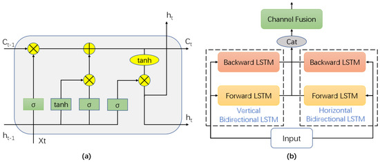
Figure 2.
(a) The specific structure of LSTM layer (b) The figure outlines the BiLSTM2D layer.
The LSTM [42] has an input gate , a forget gate , and an output gate . Where the input gate controls the storage of the input, the forget gate controls the forgetting of the previous cell state, and the output gate controls the cell output of the current cell state . As a review, the original LSTM is formulated as:
where is the Hadamard product, is the offset, are the weight matrices.
A BiLSTM consists of two LSTMs, which is formulated as:
where is the input series, is the rearrangement of in reverse order, and h is a 2D dimensional vector output.
Consisting of a vertical BiLSTM and a horizontal BiLSTM, the BiLSTM2D layers are a technique for efficiently mixing 2D spatial information. Let be the input of the Sequencer module, the BiLSTM2D can be formulated as:
where and can be viewed as a set of sequences, and is the fully-connected layer with weight .
In this process, X is the input 2D-patches, and its horizontal and vertical directions are treated separately, as sequences, as input to the LSTM.
Figure 3 demonstrates that the Transformer block contains multi-head attention, while the Sequencer module contains BiLSTM2D. In place of the multi-head self-attention in the Transformer block, the Sequencer module uses BisLSTM2D, as seen in Figure 3. Multi-head self-attention is thought to have had a significant role in the success of the Transformer. In contrast, multi-head self-attention is less memory and parameter efficient than LSTM, which is also equally capable of learning long-term dependencies. The Sequencer module is utilized in this case to extract additional discriminative spatial features. Specifically, the output, , for the previous module does not change its size in this module.
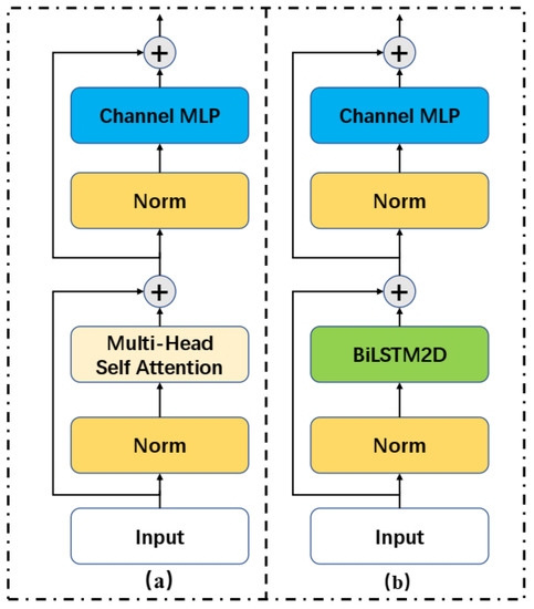
Figure 3.
(a) The Transformer block consists of multi-head attention (b) The Sequencer module consists of BiLSTM2D.
2.4. Auxiliary Classification Module
We suggest the Auxiliary Classification (AC) module, which is based on further extracting feature information and minimizing the number of parameters in fully connected layers. The AC module, the final module in the proposed model, consists of two 2D-convolution layers, a flattened layer and a fully connected layer. A BN layer, followed by a relu non-linear activation function, comes after each convolution layer. Direct classification will not be as successful as it could be after the previous two modules, despite the fact that numerous discriminative features have been retrieved and the patch size is still quite high. As a result, two 2D convolutional layers are utilized to reduce the size of the patches and the number of parameters. These layers’ convolutional kernel sizes are and , with 128 and 256 kernels, respectively. The last input channel in the last fully connected layer is 256 if the initial input patch size is . Finally, the label will be expressed as the predicted category of the sample after passing the softmax function of the AC module the highest probability value.
3. Experiment and Analysis
3.1. Hyperspectral Image Datasets Description
To examine the effectiveness and stability of our suggested SquconvNet model, we take into account three publicly available standard hyperspectral image datasets: Indian Pines (IP), University of Pavia (UP), and the Salians Scene (SA). The three datasets are summarized in Table 1.

Table 1.
Summary of the Characteristics of the IP, the UP, and the SA Datasets.
3.1.1. Indian Pines Dataset (IP)
The IP dataset was acquired by the AVIRIS sensor in northwest Indiana, and consists of 145 × 145 pixels and 224 spectral reflectance bands in the wavelength range 400 nm to 2500 nm, 24 of which, covering the region of water absorption, have been eliminated. Figure 4 depicts the false-color image and the image of the real world. For training, we randomly chose 30% of the data, and for testing, we randomly chose the remaining 70%. The category names, training samples, test samples, and the number of samples per category are listed in Table 2.
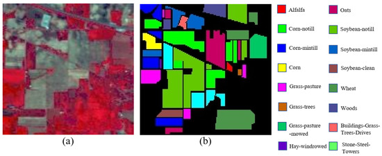
Figure 4.
Indian Pines dataset. (a) False-color image; (b) Ground Truth.
Table 2.
Training and Test Samples for the IP Dataset.
3.1.2. University of Pavia Dataset (UP)
The UP dataset includes imagery of pixels, 103 spectral depths, and a wavelength range of , and was collected by the ROSIS sensor during a flight campaign above Pavia University. There are 42,776 labeled pixels altogether, divided into nine classes of urban land-cover. Figure 5 displays the ground truth image and the false-color image. In the UP dataset, the entire set is divided into two separate datasets at random, with 10% of the samples utilized for training and the remaining 90% for classification evaluation. Table 3 provides further details on each category as well as general information.
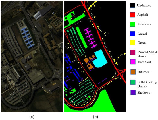
Figure 5.
University of Pavia dataset. (a) False-color image; (b) Ground Truth.
Table 3.
Training and Test Samples for UP.
3.1.3. Salians Scene Dataset (SA)
The SA dataset, acquired by the AVRIS sensor, consists of 512 × 217 spatial sizes and 224 spectral depths in the wavelength range of 360 to 2500 nm; 20 of the spectral bands, spanning the region of water absorption, have been eliminated. With the category names, training samples, test samples, and the number of samples per category indicated in Table 4, the false-color image and ground truth map are shown in Figure 6 along with the false-color image itself. Of the samples, 10% are randomly chosen for training and the remaining 90% are used for the classification evaluation.
Table 4.
Training and Testing Samples for SA.
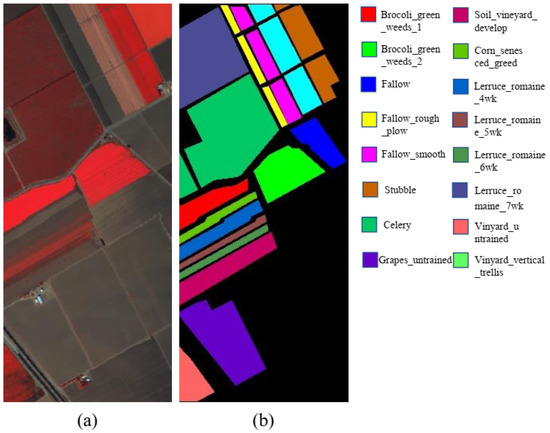
Figure 6.
Salians Scene dataset. (a) False-color image; (b) Ground Truth.
3.2. Experimental Settings
In order to make a fair comparison, both our proposed model and the compared methods were tested in the PyTorch environment on a GPU server equipped with an NVIDIA GeForce GTX 3060 12 GB. With a 256-miniature batch size, we decided to use the Adam optimizer, an optimizer with an adaptable learning rate, to improve the proposed model. According to classification performance, is chosen as the initial learning rate. There are 100 training epochs applied to each dataset. The 3D patches of for IP, and for UP and SA, are used for a fair comparison. To test the performance of our experiment, four important and common measurements are used: each class accuracy, the Overall Accuracy (OA), the Average Accuracy (AA), and the Kappa Coefficient (Kappa/k). To reduce the error associated with the randomly selected training samples, each model is run ten times to compute the average accuracy and standard deviation.
3.3. Experimental and Evaluation on Three Datasets
For a better demonstration of the superiority and stability of the proposed SquconvNet, it is compared with some representative methods: Resnet [27], 3D-CNN [25], SSRN [26], HybridSN [29], SPRN [43], and SSFTT [39]. For the Resnet, we use an optimal method, that is consistent with our model. The 3D-CNN, SSRN, HybridSN, SPRN, and SSFTT are set up as described in their corresponding references.
3.3.1. Experiment on IP Dataset
The methods of each classification are shown in Table 5. The table highlights the optimal outcomes. Particularly, HybirdSN, 3D-CNN, Resnet, etc., fared worse than our suggested method in order of best average OA value, which was 99.87%. Additionally, the performance of our proposed method is the best. The differences between the mean and the suboptimal methods of the proposed method for the evaluation of the OA, AA, and Kappa are +0.1, +0.24, and +0.11, respectively, as shown in Table 5. Additionally, the standard deviation of our proposed method is also the smallest, demonstrating our method’s higher level of stability. But it is important to remember that SSRN and SPRN’s volatility is what led to their poor classification performance. In our ten studies, the best OA achieved by SSRN and SPRN were 99.87% and 99.72%, respectively. In comparison to Resnet and SSFTT, both methods have a higher upper bound, but due to the high sample imbalance in the IP dataset, their average effectiveness is very low. The deep learning-based methods discussed above have all achieved quite good results, particularly HybridSN, based on 3D-2D convolutional architecture. However, convolutional neural networks have difficulties in classifying when the ground is irregularly shaped. In terms of the convolutional architecture, our proposed SquconvNet complements the convolution layer; by transmitting “memory” information in the horizontal and vertical directions, it is possible to overcome, to a certain extent, the convolution kernel’s inability to capture all the features in the convolution layer due to the uneven shape of the ground. For the SSFTT based on the convolution-Transformer framework, even if it can supplement the inadequacy of the global information extraction of the convolutional layer, it is also constrained by the issue that the Transformer finds it challenging to perform better on tiny data samples and has a constrained accuracy. The classification map of Ground Truth and all methods is shown in Figure 7a–h. The classification map illustrates how our proposed model produces a classification map that is not only smoother but also better in terms of texture and edge features. This demonstrates even more how effective Sequencer is at handling unusual ground forms. The proposed method SquconvNet, and the HybridSN-based classification map, outperform other methods in terms of visual performance. In conclusion, on the IP dataset, our proposed method of merging 3D-2DCNN and LSTM2D outperforms its rivals in terms of accuracy and stability.
Table 5.
Results of the various methods for IP using 30% training data (Highest performance is in Boldface).
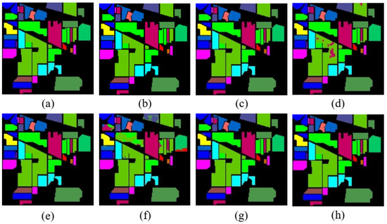
Figure 7.
Classification map of various methods for IP (a) Ground Truth, (b) Resnet, (c) 3D-CNN, (d) SSRN, (e) HybridSN, (f) SPRN, (g) SSFTT, (h) SquconvNet.
3.3.2. Experimental on UP Dataset
The average OA, AA, and Kappa (k) on the PU dataset are shown in Table 6 along with their standard deviations. Overall, the proposed SquconvNet performs better in terms of OA, AA, and Kappa than all the other methods utilized for comparison. Our method performs best in eight of the nine categories, and the standard deviation for these eight categories is the lowest of any method. On the UP dataset, the proposed method achieved an excellent OA performance of 99.93%, an improvement of +0.24 over the less-than-ideal method SSRN. On the PU dataset, 3D-CNN, SSRN, HybridSN, and SSFTT all outperformed Resnet and SPRN. With the minimum standard deviation of all the methods, the proposed SquconvNet has also shown an addition in stability. The classification maps of the UP dataset using Ground Truth and several of the methods is shown in Figure 8. Our suggested model performs better on this dataset. This outcome, from the accuracy level, is difficult to explain. It is clear that the UP dataset’s distribution is less homogeneous, and its ground shape is more erratic, than for the IP dataset. As a result, other methods have trouble in capturing discriminative features. However, the Sequencer created by LSTM performs better in the results, and is more resistant to ground shape anomalies. Additionally, the classification map’s shape is smoother, includes less noise, and has clearer bounds. Resnet and SPRN, in contrast, find it difficult to extract the most discriminative feature information, and as a result have more salt-pepper noise and incorrectly categorized area blocks. Despite having nice visual effects, the other methods still contain a lot of point noise.
Table 6.
Results of various methods for UP using 10% training data (Highest performance is in Boldface).
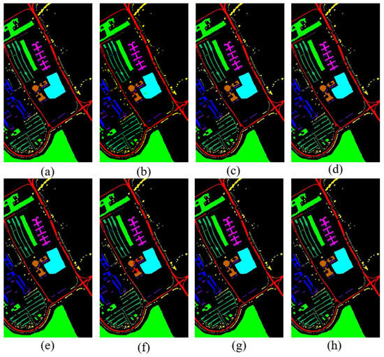
Figure 8.
Classification map of various methods for UP (a) Ground Truth, (b) Resnet, (c) 3D-CNN, (d) SSRN, (e) HybridSN, (f) SPRN, (g) SSFTT, (h) SquconvNet.
3.3.3. Experiment on SA Dataset
Table 7 displays the classification results for several networks utilizing 10% training data on the Salinas Scene Dataset. Due to instabilities and limited abilities to extract features, Resnet and SPRN perform badly, as indicated in Table 7. In contrast, the 3D-CNN, SSRN, HybridSN, and SSFTT algorithms all extracted Spectral-Spatial features with the aid of 3D-convolution, and obtained better classification results. However, they can still be made more accurate and consistent. Our proposed method achieves a mean of 99.99 on OA, AA, and Kappa, while having a lower standard deviation, thanks to the combination of 3D-2D convolution and Sequencer2D block. The classification map of the SA dataset using Ground Truth and several methods is shown in Figure 9. With large noise levels and subsequent blocks of classification mistakes, the performance of the related classification maps obtained by Resnet and SPRN was subpar. Improved results were obtained, less point noise was present, and there was better continuity between different object classes with 3D-CNN, SSRN, and HybridSN. Overall, nevertheless, our suggested approach has less point noise and smoother bounds. Table 7 makes it clear that practically all of the compared methods attain good accuracies. In fact, because there are more data and the ground is flatter, it is a very simple dataset to classify. Using only 30% of the training dataset, the HybridSN authors achieved 100% accuracy. However, in order to reduce the expense of manual annotation, we anticipate using fewer training datasets. We used 10% of the training dataset in the experiment to get an accuracy rate that was extremely close to 100%. This is not due to the overfitting phenomenon, rather, the model we suggested is superior at extracting spectral-spatial features.
Table 7.
Results of various methods for SA using 10% training data (Highest performance is in Boldface).
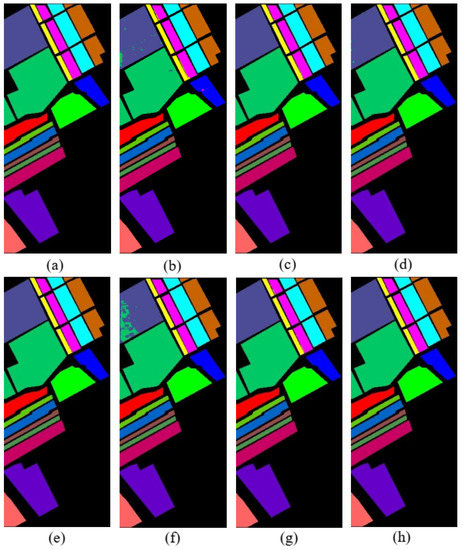
Figure 9.
Classification map of various methods for SA (a) Ground Truth, (b) Resnet, (c) 3D-CNN, (d) SSRN, (e) HybridSN, (f) SPRN, (g) SSFTT, (h) SquconvNet.
3.4. Learning Rate Experiment
An essential hyperparameter that influences how well the model fits, is the initial learning rate. In this experiment, unlike in other experiments, our dataset is divided into a 20% training set, a 10% validation set, and a 70% test set. And the results of this experiment are given by the validation set. Each of the following initial learning rates are set to 0.0001, 0.0005, 0.001, 0.005, 0.01, and 0.05 for the purposes of our experimental investigation. Figure 10 shows the classification outcomes for the IP datasets at various speeds. The best initial learning rate is 0.001 and the suboptimal initial learning rate is 0.0005, as seen in Figure 10. We set the initial learning rate for other experiments to 0.001 based on the classification results.
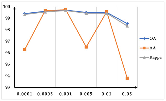
Figure 10.
The OA, AA, and Kappa of IP at different learning rates.
4. Discussion
We initially talk about the effects of the three modules on the three datasets in this section (ablation experiment). Finally, we conduct comparison experiments for a number of relatively advanced methods, as well as the proposed method, to compare training time, testing time, and parameter number.
4.1. Discussion on the Ablation Experiment
To better explore the efficiency of each SquconvNet network component, a series of ablation experiments are conducted utilizing three datasets. SDB-CNN, 3D-2DCNN, SS-SDB, and our proposed SquconvNet are four combinations we set up based on three modules. An example of their combination, and their best classification results on the IP dataset, are shown in Table 8. The methods based on the SDB and SSFE modules produce the worst outcomes. The best accuracy is attained by the proposed method. Additionally, for each of the four methods, we try training with fewer data to explore the stability of the model methods. On the three standard datasets, Figure 11, Figure 12 and Figure 13 show the overall accuracy of each of the four methods. On 5% of the training dataset for the IP dataset, SquconvNet outperforms SDB-CNN and SS-SDB. This is because there are not enough training samples for some classes to learn features with effective discriminative power due to the significant imbalance of samples (such as class.9) in the IP dataset. The experimental results also show that when the data are balanced and sufficient, the technique we suggest can produce the best results. It shows that, while our proposed method can withstand an imbalance caused by insufficient data, it loses effectiveness when the amount of data falls below a particular threshold. SDB-CNN has demonstrated a comparatively good performance while dealing with less data. When there is a small amount of data, we speculate that spatial information may be more significant than spectral information in our proposed model. Additionally, the model made up of 3D-CNN and 2D-CNN had the worst outcome. We speculate that in the case of small data, it might be brought about by the model’s poor generalization ability, brought about by 3D-CNN’s excessive emphasis on spectral information.
Table 8.
Ablation analysis of the proposed methods on the IP dataset with 30% labeled samples.
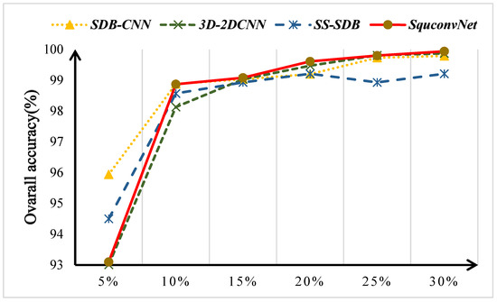
Figure 11.
The Overall Accuracy of the different proposed models on the IP dataset at different training samples.
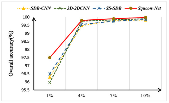
Figure 12.
The Overall Accuracy of the different proposed models on the UP dataset at different training samples.
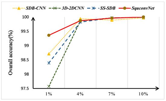
Figure 13.
The Overall Accuracy of the different proposed models on the SA dataset at different training samples.
4.2. Discussion on the Time Cost
The training time, test time, and total number of parameters for the 3D-CNN, SSRN, HybridSN, SSFTT, and SquconvNet are listed in Table 9. The slowest training speed is shown by SSRN using deep residuals. Additionally, 3D-CNN, SSRN, and HybridSN all struggle, with lengthy training and testing periods. Furthermore, the last three fully connected layers of HybridSN have resulted in an excessive number of its overall parameters, overburdening the system with parameters. SSFTT provides speed benefits, albeit at the expense of accuracy. SquconvNet increases training speed by at least twelve times and testing speed by at least four times over SSRN. SquconvNet reduced the training time for UP and SA by a factor of three and a factor of nine, respectively, when compared to HybridSN. SquconvNet has around six times fewer parameters than HybridSN, and is two to three times larger than SSRN in terms of parameter number. Furthermore, there has been a significant improvement in the classification accuracy and stability. As a result, the proposed method is useful and has promising application possibilities.
Table 9.
Training and Test time of different methods on three datasets.
5. Conclusions
This article suggests applying a hybrid SquconvNet to HSI classification that combines a 3D convolution layer, a 2D convolution layer, and a BiLSTM2D layer. The Spectral-Spatial Feature Extraction Module, the Sequencer Module, and the Auxiliary Classification Module make up the methodology. We suggest using the Sequencer based of LSTM as a supplement to the convolutional neural network in order to address its shortcomings. On three freely accessible and publicly accessible hyperspectral remote image datasets, we conduct numerous compared experiments and this method is shown to improve classification accuracy, classification speed, and stability effectively and efficiently in the experiments. When compared to conventional convolutional methods, our new method efficiently counters classification mistakes caused by erratic ground forms. The proposed method obtains average accuracies of 99.87%, 99.93%, and 99.99% on the three standard public datasets.
Additionally, we put forward the theory that, in the context of small data, spatial information may be more significant than spectral information in our proposed method. In the upcoming phase of our research, based on the SquconvNet, we intend to investigate the validity of this hypothesis under small-sample learning settings, as well as the viability of substituting 3D Sequencer for convolutional layers.
Author Contributions
Conceptualization, B.L. and Q.-W.W.; methodology, B.L. and J.-H.L.; software, Q.-W.W. and J.-H.L.; validation, B.L., Q.-W.W., J.-H.L., E.-Z.Z. and R.-Q.Z.; formal analysis, B.L., Q.-W.W., J.-H.L., E.-Z.Z. and R.-Q.Z.; writing—original draft preparation, J.-H.L., B.L. and Q.-W.W.; writing—review and editing, B.L., J.-H.L., Q.-W.W., E.-Z.Z. and R.-Q.Z. All authors have read and agreed to the published version of the manuscript.
Funding
This research was funded by the Start-up research projects of Shantou University (NTF19016).
Data Availability Statement
The datasets presented in this paper is available through https://www.ehu.eus/ccwintco/index.php/Hyperspectral_Remote_Sensing_Scenes, accessed on 11 November 2022.
Conflicts of Interest
The authors declare no conflict of interest.
References
- Prasad, S.; Bruce, L.M. Limitations of Principal Components Analysis for Hyperspectral Target Recognition. IEEE Geosci. Remote Sens. Lett. 2008, 5, 625–629. [Google Scholar] [CrossRef]
- Piiroinen, R.; Heiskanen, J.; Maeda, E.; Viinikka, A.; Pellikka, P. Classification of Tree Species in a Diverse African Agroforestry Landscape Using Imaging Spectroscopy and Laser Scanning. Remote Sens. 2017, 9, 875. [Google Scholar] [CrossRef]
- Chen, S.Y.; Lin, C.S.; Tai, C.H.; Chuang, S.J. Adaptive Window-Based Constrained Energy Minimization for Detection of Newly Grown Tree Leaves. Remote Sens. 2018, 10, 96. [Google Scholar] [CrossRef]
- Zhang, H.; Zhang, B.; Chen, Z.C.; Huang, Z.H. Vicarious Radiometric Calibration of the Hyperspectral Imaging Microsatellites SPARK-01 and-02 over Dunhuang, China. Remote Sens. 2018, 10, 120. [Google Scholar] [CrossRef]
- Tane, Z.; Roberts, D.; Veraverbeke, S.; Casas, A.; Ramirez, C.; Ustin, S. Evaluating Endmember and Band Selection Techniques for Multiple Endmember Spectral Mixture Analysis using Post-Fire Imaging Spectroscopy. Remote Sens. 2018, 10, 389. [Google Scholar] [CrossRef]
- Ni, L.; Wub, H. Mineral Identification and Classification by Combining Use of Hyperspectral VNIR/SWIR and Multispectral TIR Remotely Sensed Data. In Proceedings of the IGARSS 2019—2019 IEEE International Geoscience and Remote Sensing Symposium, Yokohama, Japan, 28 July–2 August 2019; pp. 3317–3320. [Google Scholar]
- Li, J.; Bioucas-Dias, J.M.; Plaza, A. Spectral-Spatial Classification of Hyperspectral Data Using Loopy Belief Propagation and Active Learning. IEEE Trans. Geosci. Remote Sens. 2013, 51, 844–856. [Google Scholar] [CrossRef]
- Zhang, L.; Zhong, Y.; Huang, B.; Gong, J.; Li, P. Dimensionality reduction based on clonal selection for hyperspectral imagery. IEEE Trans. Geosci. Remote Sens. 2007, 45, 4172–4186. [Google Scholar] [CrossRef]
- Brown, A.J.; Sutter, B.; Dunagan, S. The MARTE VNIR Imaging Spectrometer Experiment: Design and Analysis. Astrobiology 2008, 8, 1001–1011. [Google Scholar] [CrossRef]
- Brown, A.J.; Hook, S.J.; Baldridge, A.M.; Crowley, J.K.; Bridges, N.T.; Thomson, B.J.; Marion, G.M.; de Souza, C.R.; Bishop, J.L. Hydrothermal formation of Clay-Carbonate alteration assemblages in the Nil Fossae region of Mars. Earth Planet. Sci. Lett. 2010, 297, 174–182. [Google Scholar] [CrossRef]
- Zhu, J.S.; Hu, J.; Jia, S.; Jia, X.P.; Li, Q.Q. Multiple 3-D Feature Fusion Framework for Hyperspectral Image Classification. IEEE Trans. Geosci. Remote Sens. 2018, 56, 1873–1886. [Google Scholar] [CrossRef]
- Chen, Y.S.; Lin, Z.H.; Zhao, X.; Wang, G.; Gu, Y.F. Deep Learning-Based Classification of Hyperspectral Data. IEEE J. Sel. Top. Appl. Earth Obs. Remote Sens. 2014, 7, 2094–2107. [Google Scholar] [CrossRef]
- Lavanya, A.; Sanjeevi, S. An Improved Band Selection Technique for Hyperspectral Data Using Factor Analysis. J. Indian Soc. Remote Sens. 2013, 41, 199–211. [Google Scholar] [CrossRef]
- Bandos, T.V.; Bruzzone, L.; Camps-Valls, G. Classification of Hyperspectral Images With Regularized Linear Discriminant Analysis. IEEE Trans. Geosci. Remote Sens. 2009, 47, 862–873. [Google Scholar] [CrossRef]
- Ye, Q.; Yang, J.; Liu, F.; Zhao, C.; Ye, N.; Yin, T. L1-Norm Distance Linear Discriminant Analysis Based on an Effective Iterative Algorithm. IEEE Trans. Circuits Syst. Video Technol. 2018, 28, 114–129. [Google Scholar] [CrossRef]
- Villa, A.; Benediktsson, J.A.; Chanussot, J.; Jutten, C. Independent Component Discriminant Analysis for hyperspectral image classification. In Proceedings of the 2010 2nd Workshop on Hyperspectral Image and Signal Processing: Evolution in Remote Sensing, Reykjavik, Iceland, 14–16 June 2010; pp. 1–4. [Google Scholar]
- Villa, A.; Benediktsson, J.A.; Chanussot, J.; Jutten, C. Hyperspectral Image Classification With Independent Component Discriminant Analysis. IEEE Trans. Geosci. Remote Sens. 2011, 49, 4865–4876. [Google Scholar] [CrossRef]
- Melgani, F.; Bruzzone, L. Classification of hyperspectral remote sensing images with support vector machines. IEEE Trans. Geosci. Remote Sens. 2004, 42, 1778–1790. [Google Scholar] [CrossRef]
- Gislason, P.O.; Benediktsson, J.A.; Sveinsson, J.R. Random Forests for land cover classification. Pattern Recognit. Lett. 2006, 27, 294–300. [Google Scholar] [CrossRef]
- Haut, J.M.; Paoletti, M.; Plaza, J.; Plaza, A. Cloud implementation of the K-means algorithm for hyperspectral image analysis. J. Supercomput. 2017, 73, 514–529. [Google Scholar] [CrossRef]
- Tarabalka, Y.; Fauvel, M.; Chanussot, J.; Benediktsson, J.A. SVM- and MRF-Based Method for Accurate Classification of Hyperspectral Images. IEEE Geosci. Remote Sens. Lett. 2010, 7, 736–740. [Google Scholar] [CrossRef]
- Li, T.; Zhang, J.; Zhang, Y. Classification of hyperspectral image based on deep belief networks. In Proceedings of the 2014 IEEE International Conference on Image Processing (ICIP), Paris, France, 27–30 October 2014; pp. 5132–5136. [Google Scholar]
- Hu, W.; Huang, Y.; Wei, L.; Zhang, F.; Li, H. Deep Convolutional Neural Networks for Hyperspectral Image Classification. J. Sens. 2015, 2015, 258619. [Google Scholar] [CrossRef]
- Zhao, W.; Du, S. Spectral–Spatial Feature Extraction for Hyperspectral Image Classification: A Dimension Reduction and Deep Learning Approach. IEEE Trans. Geosci. Remote Sens. 2016, 54, 4544–4554. [Google Scholar] [CrossRef]
- Chen, Y.; Jiang, H.; Li, C.; Jia, X.; Ghamisi, P. Deep Feature Extraction and Classification of Hyperspectral Images Based on Convolutional Neural Networks. IEEE Trans. Geosci. Remote Sens. 2016, 54, 6232–6251. [Google Scholar] [CrossRef]
- Zhong, Z.; Li, J.; Luo, Z.; Chapman, M. Spectral–Spatial Residual Network for Hyperspectral Image Classification: A 3-D Deep Learning Framework. IEEE Trans. Geosci. Remote Sens. 2018, 56, 847–858. [Google Scholar] [CrossRef]
- He, K.; Zhang, X.; Ren, S.; Sun, J. Deep Residual Learning for Image Recognition. In Proceedings of the 2016 IEEE Conference on Computer Vision and Pattern Recognition (CVPR), Las Vegas, NV, USA, 27–30 June 2016; pp. 770–778. [Google Scholar]
- Paoletti, M.E.; Haut, J.M.; Fernandez-Beltran, R.; Plaza, J.; Plaza, A.J.; Pla, F. Deep Pyramidal Residual Networks for Spectral–Spatial Hyperspectral Image Classification. IEEE Trans. Geosci. Remote Sens. 2019, 57, 740–754. [Google Scholar] [CrossRef]
- Roy, S.K.; Krishna, G.; Dubey, S.R.; Chaudhuri, B.B. HybridSN: Exploring 3-D–2-D CNN Feature Hierarchy for Hyperspectral Image Classification. IEEE Geosci. Remote Sens. Lett. 2020, 17, 277–281. [Google Scholar] [CrossRef]
- Li, J.J.; Zhao, X.; Li, Y.S.; Du, Q.; Xi, B.B.; Hu, J. Classification of Hyperspectral Imagery Using a New Fully Convolutional Neural Network. IEEE Geosci. Remote Sens. Lett. 2018, 15, 292–296. [Google Scholar] [CrossRef]
- Tun, N.L.; Gavrilov, A.; Tun, N.M.; Trieu, D.M.; Aung, H. Hyperspectral Remote Sensing Images Classification Using Fully Convolutional Neural Network. In Proceedings of the 2021 IEEE Conference of Russian Young Researchers in Electrical and Electronic Engineering (ElConRus), St. Petersburg, Moscow, 26–29 January 2021; pp. 2166–2170. [Google Scholar]
- Bi, X.J.; Zhou, Z.Y. Hyperspectral Image Classification Algorithm Based on Two-Channel Generative Adversarial Network. Acta Opt. Sin. 2019, 39, 1028002. [Google Scholar] [CrossRef]
- Xue, Z.X. Semi-supervised convolutional generative adversarial network for hyperspectral image classification. IET Image Process. 2020, 14, 709–719. [Google Scholar] [CrossRef]
- Hong, D.; Gao, L.; Yao, J.; Zhang, B.; Plaza, A.; Chanussot, J. Graph Convolutional Networks for Hyperspectral Image Classification. IEEE Trans. Geosci. Remote Sens. 2021, 59, 5966–5978. [Google Scholar] [CrossRef]
- Dosovitskiy, A.; Beyer, L.; Kolesnikov, A.; Weissenborn, D.; Zhai, X.; Unterthiner, T.; Dehghani, M.; Minderer, M.; Heigold, G.; Gelly, S. An image is worth 16x16 words: Transformers for image recognition at scale. arXiv 2020, arXiv:2010.11929. [Google Scholar]
- He, X.; Chen, Y.S.; Lin, Z.H. Spatial-Spectral Transformer for Hyperspectral Image Classification. Remote Sens. 2021, 13, 498. [Google Scholar] [CrossRef]
- Qing, Y.H.; Liu, W.Y.; Feng, L.Y.; Gao, W.J. Improved Transformer Net for Hyperspectral Image Classification. Remote Sens. 2021, 13, 2216. [Google Scholar] [CrossRef]
- Hong, D.F.; Han, Z.; Yao, J.; Gao, L.R.; Zhang, B.; Plaza, A.; Chanussot, J. SpectralFormer: Rethinking Hyperspectral Image Classification With Transformers. Ieee Trans. Geosci. Remote Sens. 2022, 60, 5518615. [Google Scholar] [CrossRef]
- Sun, L.; Zhao, G.; Zheng, Y.; Wu, Z. Spectral–Spatial Feature Tokenization Transformer for Hyperspectral Image Classification. IEEE Trans. Geosci. Remote Sens. 2022, 60, 5522214. [Google Scholar] [CrossRef]
- Zhu, J.; Fang, L.; Ghamisi, P. Deformable convolutional neural networks for hyperspectral image classification. IEEE Geosci. Remote Sens. Lett. 2018, 15, 1254–1258. [Google Scholar] [CrossRef]
- Tatsunami, Y.; Taki, M. Sequencer: Deep LSTM for Image Classification. arXiv 2022, arXiv:2205.01972. [Google Scholar]
- Hochreiter, S.; Schmidhuber, J. Long short-term memory. Neural Comput. 1997, 9, 1735–1780. [Google Scholar] [CrossRef]
- Zhang, X.; Shang, S.; Tang, X.; Feng, J.; Jiao, L. Spectral Partitioning Residual Network With Spatial Attention Mechanism for Hyperspectral Image Classification. IEEE Trans. Geosci. Remote Sens. 2022, 60, 5507714. [Google Scholar] [CrossRef]
Disclaimer/Publisher’s Note: The statements, opinions and data contained in all publications are solely those of the individual author(s) and contributor(s) and not of MDPI and/or the editor(s). MDPI and/or the editor(s) disclaim responsibility for any injury to people or property resulting from any ideas, methods, instructions or products referred to in the content. |
© 2023 by the authors. Licensee MDPI, Basel, Switzerland. This article is an open access article distributed under the terms and conditions of the Creative Commons Attribution (CC BY) license (https://creativecommons.org/licenses/by/4.0/).