Abstract
Monitoring land surface phenology plays a fundamental role in quantifying the impact of climate change on terrestrial ecosystems. Shifts in land surface spring phenology have become a hot spot in the field of global climate change research. While numerous studies have used satellite data to capture the interannual variation of the start of the growing season (SOS), the understanding of spatiotemporal performances of SOS needs to be enhanced. In this study, we retrieved the annual SOS from the Moderate Resolution Imaging Spectroradiometer (MODIS) two-band enhanced vegetation index (EVI2) time series in the conterminous United States from 2001 to 2021, and explored the spatial and temporal patterns of SOS and its trend characteristics in different land cover types. The performance of the satellite-derived SOS was evaluated using the USA National Phenology Network (USA-NPN) and Harvard Forest data. The results revealed that SOS exhibited a significantly delayed trend of 1.537 days/degree (p < 0.01) with increasing latitude. The timing of the satellite-derived SOS was significantly and positively correlated with the in-situ data. Despite the fact that the overall trends were not significant from 2001 to 2021, the SOS and its interannual variability exhibited a wide range of variation across land cover types. The earliest SOS occurred in urban and built-up land areas, while the latest occurred in cropland areas. In addition, mixed trends in SOS were observed in sporadic areas of different land cover types. Our results found that (1) warming hiatus slows the advance of land surface spring phenology across the conterminous United States under climate change, and (2) large-scale land surface spring phenology trends extraction should consider the potential effects of different land cover types. To improve our understanding of climate change, we need to continuously monitor and analyze the dynamics of the land surface spring phenology.
1. Introduction
Phenology usually refers to the timing of recurring biological phases and is sensitive to a series of biotic and abiotic conditions and changes [1,2,3]. Land surface phenology typically tracks seasonal dynamics in the vegetated land surface and is a key indicator of biosphere feedbacks to the climate system [4,5]. Land surface phenology influences the exchange of carbon, water and energy between vegetation and the atmosphere by controlling seasonal changes in ecosystem structure and function [6]. As a result, the timing of phenological events (e.g., green-up, flowering, and dormancy) is commonly used in studies of terrestrial ecosystems to quantify the effects of climate change on vegetation growth [7,8,9,10]. Global warming is dramatically altering land surface phenology and its interactions [11,12,13,14]. Tracking phenological changes at large scales (e.g., continental and global scales) is key to understanding ecosystem condition and change [4]. At present, phenology research is of increasing public interest [15], as it is critical for understanding how terrestrial ecosystems are responding to climate change [16].
Rapidly developing satellite remote sensing technology has supported continental and global scale phenology observations in the past decades [9,17]. A range of satellite images, such as Landsat, Sentinel, Systeme Probatoire d’Observation de la Terre (SPOT), Advanced Very High Resolution Radiometer (AVHRR), and Moderate Resolution Imaging Spectroradiometer (MODIS), provide increasingly new perspectives and opportunities for large scale phenology observations [18]. The basic principle of land surface phenology retrieval based on satellite data is to extract key phenological metrics in the vegetation growth cycle, such as the start of the growing season (SOS), the end of the growing season (EOS), and growing season length (GSL), by identifying inflection points in the time series of remote sensing observations [19,20,21,22]. Various methods have been developed to retrieve land surface phenology based on this principle. For example, several studies extracted dates of phenological metrics based on thresholds of seasonal amplitudes in vegetation index time series [23,24]. The derivative method identifies key phenophases based on the change rate of points in the vegetation index time series [25,26,27]. The model fitting method uses a smoothing model function to fit vegetation index time series and then extracts phenological metrics according to the characteristic points of the fitted curve. Common fitting methods include polynomials, Logistic functions and Gaussian functions [28,29,30]. The dates of phenological metrics retrieved using different methods vary considerably [31]. Our previous study compared the performances of multiple phenology retrieval methods based on MODIS data and ultimately found that the SOS extracted using the first-order derivative method and the EOS extracted using the polynomial fitting method were the most consistent with ground-based phenology observations [32].
Changes in the timing of land surface spring phenology are closely related to the climate change and have attracted a lot of attention from the scientific community [33]. Since the 1980s, numerous studies have shown that climate warming leads to earlier SOS and later EOS in terrestrial ecosystems, resulting in longer GSL [4,9,34,35]. However, the long-term trends of spring phenology were not fully consistent at the regional scale. For example, Zhang et al. [36] analyzed spring phenology trends in the conterminous United States from 1982 to 2005 based on AVHRR data and showed that SOS was significantly advanced in the Northeast, Mid-Atlantic, and Upper Midwest, while significantly delayed in the Southeast of the conterminous United States. In another study that extracted land surface phenology based on AVHRR normalized difference vegetation index (NDVI) time series, SOS showed a significantly delayed trend in the Midwestern Corn Belt, while there was a significantly advanced trend in the Northeast of the United States from 1982 to 2012 [37]. Fu et al. [38] found that the SOS in Western Central Europe showed a significantly advanced trend from 1982 to 1999, while the trend was reversed between 2000 and 2011. Zhang et al. [39] found that SOS showed a significantly delayed trend between 1982 and 2014 across croplands of the Midwest and Northern Great Plains of the United States. This inconsistency between studies may be due to multiple reasons, such as different algorithms used for phenology retrieval, different methods used for trend detection, different spatial resolution of satellite data, and different study periods [4,31,32].
Therefore, satellite-derived phenological metrics need to be cross-compared with in-situ observations [40,41,42]. Currently, ground-based phenology observation networks are available in several countries and regions. For example, the USA National Phenology Network (USA-NPN) [43], the Pan European Phenology Project (PEP725) [44] and the Chinese Phenological Observation Network (CPON) [45,46,47]. In addition, flux tower observations are often used to assess the performance of satellite-derived phenological metrics [22,48,49]. It has been found that due to the mismatch in spatial scales, the phenological metrics derived from satellite data differ significantly from the ground-based observations [50]. Nevertheless, a significant positive correlation was found between satellite-derived phenological metrics and ground-based phenological records in our previous studies [31,32]. To enhance the understanding of phenology studies at different spatial scales and to accurately characterize phenology changes, it is essential to evaluate satellite-derived phenological metrics using ground-based phenological observations.
The main objective of this study was to examine the long-term trends of land surface spring phenology across the conterminous United States, and to answer the following questions: (1) What are the spatial characteristics of land surface spring phenology in the conterminous United States? and (2) What are the differences in land surface spring phenology trends on different land cover types? Answering these questions will help to develop more reliable phenological metrics that more accurately reflect the response of terrestrial ecosystems to biotic and abiotic factors under climate change, thereby informing human responses to climate change.
2. Materials and Methods
2.1. Satellite Data Acquisition
This study focused on the conterminous United States for the period 2001–2021. We used the land surface reflectance product (MOD09A1) and the land cover type product (MCD12Q1) from the MODIS satellites. MOD09A1 is an 8-day composite land surface reflectance product with a spatial resolution of 500 m. We calculated the two-band enhanced vegetation index (EVI2) [51] time series for the conterminous United States based on MOD09A1 data. MCD12Q1 is a global land cover type product containing five classification schemes with a spatial resolution of 500 m and a time step of one year. Based on the International Geosphere Biosphere Programme (IGBP) classification scheme [52] in the product (Figure 1a), we extracted the following four categories required for this study: forest (including evergreen needleleaf forests, evergreen broadleaf forests, deciduous needleleaf forests, deciduous broadleaf forests, mixed forests, closed shrublands and open shrublands), grassland (including woody savannas, savannas and grasslands), cropland (including croplands and cropland/natural vegetation mosaics), and urban and built-up land areas (Figure 1b). The MODIS data used in this study were obtained from the National Aeronautics and Space Administration (NASA) [53].
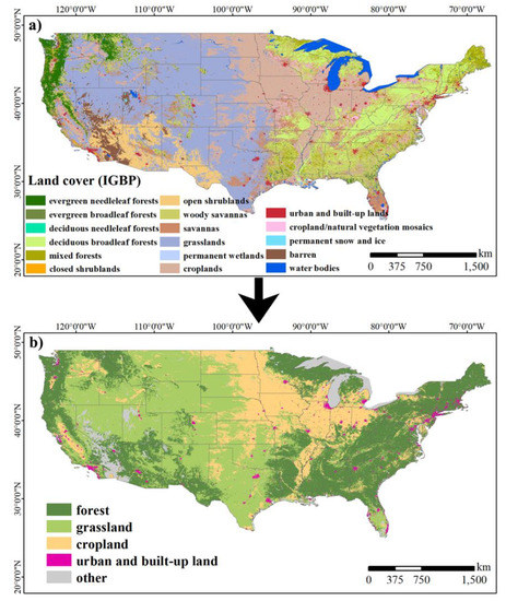
Figure 1.
Land cover types in the conterminous United States, where (a) denotes the IGBP classification scheme, and (b) denotes the four categories required for this study.
2.2. In-Situ Data Acquisition
We used ground-based phenology observation networks and flux tower observations to evaluate the performance of the satellite-derived SOS (Figure 2). The USA-NPN records phenology information for more than 400 different plant types at nearly 3,000 sites. In this study, the spring onset (i.e., the phenophase described as ‘breaking leaf buds’) of deciduous vegetation in the USA-NPN leaf phenological observation dataset was selected to evaluate the satellite-derived SOS, with a total of 5492 records available. The Harvard Forest flux tower site is located at 42.535°N, 72.185°W. All observed tree individuals are located within 1.5 km of the site and range in elevation from 335 to 365 m. We used the spring phenology observation records from Harvard Forest to assess the satellite-derived SOS.

Figure 2.
The USA-NPN sites and the Harvard Forest site used in this study.
2.3. Satellite Imagery Processing
2.3.1. Data Pre-Processing
We calculated the EVI2 in the conterminous United States from July 2000 to December 2021 based on the red and near-infrared bands of MOD09A1 land surface reflectance data. Quality control of EVI2 data is necessary due to factors such as sensors specifications, clouds, and noise. First, based on the quality assessment data for the MOD09A1 product, we removed the data identified as clouds and replaced the data identified as snow with the closest snow-free data in the EVI2 time series. Second, the median of a 7-points moving window was used to replace outliers that differ from this median by more than three standard deviations in the EVI2 time series [24]. Finally, we applied spline interpolation to the 8-day EVI2 time series to obtain the daily EVI2 time series, which was smoothed using Savitzky-Golay [54] filtering.
Notably, to simulate the complete spring green-up phase, we extended the EVI2 time series for each calendar year forward by six months. For example, we used the EVI2 time series between July 2000 and December 2001 to extract the SOS in 2001.
2.3.2. Time Series Fitting
The vegetation spring green-up phase corresponds to the period of time when EVI2 increases in a monotonous manner, that is, the sustained period of increase from local minimum to local maximum in the EVI2 time series. To eliminate slight increases in EVI2 time series unrelated to vegetation growth, we used the following heuristics: (1) the duration of the spring green-up phase should be greater than 45 days and no more than 180 days; (2) the ratio of the local maximum EVI2 to the corresponding local minimum EVI2 should be not less than 1.5, and the difference between the local maximum EVI2 and the corresponding local minimum EVI2 should be at least 0.15.
To successfully simulate vegetation growth, we fitted the EVI2 time series of vegetation spring green-up phase using a widely accepted Logistic curve fitting function [22]:
where t represents the time in days, both a and b are fitting parameters, c is the amplitude of the EVI2 time series, and m is the minimum EVI2 value.
2.4. Land Surface Spring Phenology Extraction
We used the widely accepted first-order derivative method (Figure 3) [27,28,55,56] to extract the timing of annual SOS (2001–2021) from the fitted EVI2 time series in the conterminous United States. In general, the fastest increasing point in the vegetation index time series curve indicates the beginning of vegetation growth. Here, SOS is defined as the date corresponding to the maximum slope in the fitted EVI2 curve. In other words, SOS is the date when the first local maximum occurs in the first-order derivative curve of the fitted EVI2 time series. The unit describing SOS is day of year (DOY).
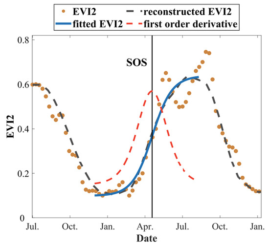
Figure 3.
The principle of first-order derivative method to extract the timing of SOS.
2.5. Accuracy Assessment and Correlation Analysis
We used the ground-based phenology network (i.e., USA-NPN) and flux tower observations (i.e., Harvard Forest data) to evaluate the satellite-derived SOS. The quantitative metrics used to assess the performance of SOS were the Pearson correlation coefficient (r) and the root mean square error (RMSE). In addition, we used a simple linear regression model to detect trends in SOS over the study period. In the model, the year is the independent variable and the satellite-derived SOS is the dependent variable.
2.6. Software
In this study, we used MATLAB R2019b and ArcGIS 10.7 for data processing, analysis and visualization.
3. Results
3.1. Spatial Distributions
Figure 4 shows the mean SOS in the conterminous United States from 2001 to 2021 retrieved using the first-order derivative method. Overall, SOS gradually advances from north to south. However, in the Great Lakes, Middle Atlantic, and Southwest of the conterminous United States, the timing of mean SOS (generally later than DOY 140) is later than in the surrounding areas, while the timing of mean SOS (generally earlier than DOY 90) in the Pacific Coast region is earlier than in the surrounding areas.
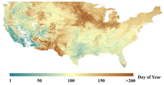
Figure 4.
Spatial distribution of 21-year mean SOS in the conterminous United States from 2001 to 2021.
The variation characteristics of the mean SOS in the latitudinal direction from 2001 to 2021 across the conterminous United States are shown in Figure 5. The standard deviation of the mean SOS was relatively stable in the latitudinal direction. The timing of mean SOS exhibited a significantly delayed trend of 1.537 days/degree (r = 0.876 **, RMSE = 6.359 days) with increasing latitude. However, the timing of mean SOS gradually advanced with increasing latitude in low-latitude (<30°N) regions.

Figure 5.
Trend of mean SOS (2001–2021) in the latitudinal direction. The light blue bar represents the standard deviation. ** denotes p < 0.01.
3.2. Assessment
As there are many outliers in the USA-NPN observations, we applied robust regression to reduce the effect of outliers. When using robust regression, satellite-derived dates of SOS were significantly correlated with dates of SOS derived from USA-NPN (r = 0.81, RMSE = 15.09 days) (Figure 6a). Figure 6b compares the satellite-derived SOS and the SOS derived from Harvard Forest using a simple linear regression method. Satellite-derived dates of SOS exhibited significant correlation with dates of SOS derived from Harvard Forest data, achieving r = 0.62 and RMSE = 4.89 days.

Figure 6.
Comparison of satellite-derived dates of SOS with in-situ data, where (a) is USA-NPN data, and (b) is Harvard Forest data. The red dashed lines denote regression lines. ** denotes p < 0.01.
3.3. Trends Analysis
To understand the long-term change characteristics of land surface spring phenology in the United States, we extracted trends (2001–2021) of annual mean SOS for four land cover types: forest, grassland, cropland, and urban and built-up land, respectively (Figure 7). From 2001 to 2021, the annual mean SOS exhibited weakly delayed trends in forest (0.03274 days/year), grassland (0.08038 days/year), cropland (0.3128 days/year), and urban and built-up land (0.1427 days/year) areas. Note that the annual mean SOS trends of all land cover types were insignificant (p > 0.05). The SOS in different land cover types exhibited a wide range of interannual variation. The SOS range was the largest in cropland areas (21.54 days) and the smallest in forest areas (12.53 days). The variation ranges of SOS in the grassland and urban and built-up land areas were 20.22 days and 15.59 days, respectively. Although the trajectories of the annual mean SOS curves for the period 2001–2012 were very close in different land cover types, the corresponding dates of SOS were significantly different, with a maximum of 34 days for the same years.
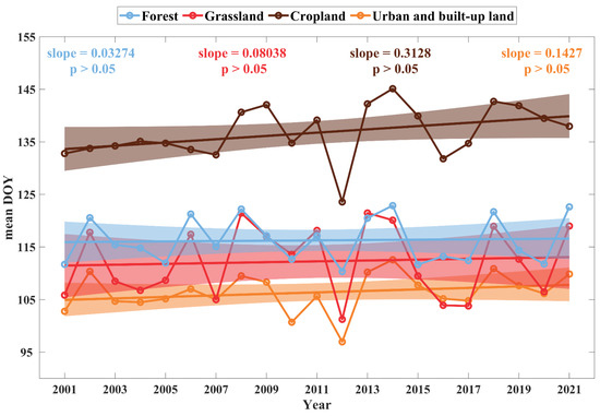
Figure 7.
Temporal trends of annual mean SOS for different land cover types (i.e., forest, grassland, cropland, and urban and built-up land) in the conterminous United States over the past two decades. The colored solid lines denote the trend lines, and the colored bars represent 95% confidence intervals.
Considering that the annual mean SOS of cropland is significantly later than the annual mean SOS of other land cover types, we extracted the temporal trend of the annual mean SOS of the study area under two scenarios (i.e., including and excluding cropland) (Figure 8). The trend was calculated at the 95% confidence level. Figure 8a shows the annual mean SOS trend from 2001 to 2021 that include cropland. The mean SOS exhibited an insignificantly delayed trend (p > 0.05) with 0.1050 days/year from 2001 to 2021. Figure 8b shows the annual mean SOS trend from 2001 to 2021 that exclude cropland. The mean SOS exhibited an insignificantly delayed trend (p > 0.05) with 0.06048 days/year over the past 21 years. The ranges of SOS interannual variation for the two scenarios were 17.52 days and 16.31 days, respectively. The annual mean SOS including cropland was generally later than the annual mean SOS excluding cropland, ranging from 2.7 to 5.4 days.
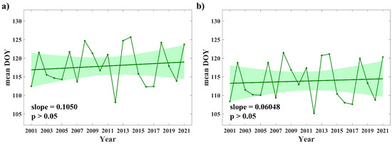
Figure 8.
Temporal trend of annual mean SOS in the conterminous United States from 2001 to 2021, (a) indicates the annual mean SOS trend when cropland is included, and (b) indicates the annual mean SOS trend when cropland is excluded. The green solid line denotes the trend line, and the bar represents 95% confidence interval.
Although no significant trends in annual mean SOS were observed for any of the four land cover types (i.e., forest, grassland, cropland, and urban and built-up land), mixed trends (either significantly advanced or delayed trends) were observed in localized areas (Figure 9). Figure 9a shows the distribution of SOS trends in the forest areas from 2001 to 2021. SOS showed significantly delayed trends (p < 0.05) in sporadic forest areas in the Pacific Coast region (e.g., Region 1) and the Southwest (e.g., Region 2), while significantly advanced trends (p < 0.05) in sporadic forest areas in the Southeast (e.g., Region 3) of the United States. Figure 9b shows the distribution of SOS trends in the grassland areas from 2001 to 2021. SOS was significantly delayed (p < 0.05) in parts of grassland areas in the Mid-west (e.g., Region 6), while was significantly advanced (p < 0.05) in parts of grassland areas in the Northern Rocky Mountain States (e.g., Region 4) and Eastern Texas (e.g., Region 5). Figure 9c shows the distribution of SOS trends in the cropland areas from 2001 to 2021. SOS showed significantly delayed trends (p < 0.05) in parts of cropland areas in the Mid-west (e.g., Region 7) and Great Lakes (e.g., Region 8) of the United States. Figure 9d shows the distribution of SOS trends in urban and built-up land areas from 2001 to 2021. Significantly delayed trends (p < 0.05) were observed in sporadic areas in various urban agglomerations (e.g., Region 9 and Region 10), while advanced trends were rarely observed.

Figure 9.
Trends distribution of SOS in four land cover types from 2001 to 2021, where (a) is forest, (b) is grassland, (c) is cropland, and (d) is urban and built-up land.
4. Discussion
In this study, we retrieved SOS for the past 20 years in the conterminous United States based on the MODIS data. The spatial distribution of SOS is closely related to climate change. Over the past few decades, significant warming occurred primarily in the Western United States, but was absent in a large portion of the East, especially in the Southeast of the conterminous United States [57,58]. One study found that the Pacific Coast region was humid and the timing of SOS was significantly earlier, while in the drier Southwest of the United States, the timing of SOS was significantly later due to less spring precipitation [4]. This finding was consistent with the results of this paper (Figure 4). In addition, our results indicated that SOS was generally later over most parts of the eastern United States, especially in areas that overlap with the agricultural belts of the United States. The later SOS in these areas may be controlled by changes in agronomic practices, such as changes in tillage practices, planting of different crop varieties, and a shift to later-emerging crops rather than earlier-emerging ones [4,39].
In the Northern Hemisphere, SOS is gradually delayed with increasing latitude. Nevertheless, SOS showed an opposite trend below 30°N (Figure 5). One possible reason is that the chilling accumulation in winter at low latitudes is not sufficient for the heat requirements of vegetation spring growth, so that the SOS is delayed [36,59]. Moreover, land surface phenology in temperate zones in the Northern Hemisphere is primarily driven by temperature, while land surface phenology in tropical zones near the equator is highly sensitive to precipitation [6,60,61].
Despite the differences in spatial scale and temporal frequency between ground and satellite observations, a study using a landscape up-scaling approach successfully demonstrated that satellite-derived phenological metrics captured intra- and inter-annual variability consistent with ground-based phenology records [41]. Table 1 presents the results of some studies that used in-situ data to assess satellite-derived SOS. Xin et al. [31] evaluated the SOS extracted from MODIS data using USA-NPN observations with r = 0.570 (p < 0.01) and RMSE = 27.41 days. Bórnez et al. [62] found a significant correlation (r = 0.630 (p < 0.01) and RMSE = 14.14 days) between the SOS derived from SPOT-VEGETATION and PROBA-V time series data and the SOS derived from USA-NPN data. Peng et al. [63] assessed the SOS retrieved from MODIS data using USA-NPN data, achieving r = 0.320 (p < 0.01) and RMSE = 34.97 days. In this study, we used USA-NPN data to evaluate the satellite-derived SOS and obtained similar results (Figure 6a). In addition, when using Harvard Forest data to evaluate satellite-derived SOS, Li et al. (r = 0.810 (p < 0.01) and RMSE = 3.5 days) [64], Tan et al. (r = 0.812 (p < 0.01) and RMSE = 11.1 days) [26] and this paper (r = 0.620 (p < 0.01) and RMSE = 4.89 days) all found that the satellite-derived SOS was strongly correlated with Harvard Forest data. Overall, ground-based phenology observations are useful for understanding remotely sensed phenological retrievals.

Table 1.
The accuracy metrics related to the assessment on SOS retrieved from satellite data using in-situ data.
In this study, we simply extracted four categories (i.e., forest, grassland, cropland, and urban and built-up land) according to the IGBP classification scheme in the MCD12Q1 product. Due to the coarse spatial resolution (500 m), MCD12Q1 is not designed to be used for mapping land cover changes [65]. The purpose of this paper is not to precisely extract the land cover types in the study area, but to simply extract the land surface spring phenology trends of representative areas in terrestrial ecosystems. For example, forests and grasslands are the dominant vegetation types on the land surface, and the vegetation phenology on cropland and urban areas is largely driven by human activities. In particular, urban heat islands and highly heterogeneous surface climate conditions differentiate the phenological characteristics of vegetation in the urban from that in surrounding areas [66,67,68]. While no significant trends in annual mean SOS were observed across the four land cover categories, there were large intra-annual differences between categories (Figure 7). Specifically, the earliest SOS occurred in the urban and built-up land areas, while the latest was in the cropland areas. The SOS of forest areas was slightly later than that of grassland areas. There may be multiple reasons for these differences. In addition to natural factors, human activities have a very important influence on the land surface spring phenology. For example, it has been found that SOS is earlier in urban areas than in the surrounding area, and that a tenfold increase in urban size leads to an earlier SOS of approximately 1.3 days [68]. Moreover, SOS in cropland areas depends on the date of human sowing, changes in tillage practices, and changes in crop varieties [4].
The concept that warming results in earlier land surface spring phenology has been widely accepted [8,11]. Nevertheless, in this study, despite the fact that SOS exhibited significantly advanced or delayed trends in sporadic areas, the annual mean SOS in the conterminous United States showed insignificant changes from 2001 to 2021. Numerous studies indicated a global warming hiatus since 1998 [69,70,71]. For example, Jeong et al. [72] found that SOS in the Northern Hemisphere advanced by 5.2 days from 1982 to 1999, but advanced by only 0.2 days from 2000 to 2008. Wang et al. [73] used long-term FLUXNET measurements to examine phenology trends in the Northern Hemisphere during warming hiatus and showed no widespread advancing (or delaying) trends in spring (or autumn) phenology. According to the Fifth Assessment Report of the Intergovernmental Panel on Climate Change (IPCC AR5) [74], the warming slowdown was due to the combined effects of long-term internal variability and natural forcing (volcanic and solar) superimposed on human-caused warming [69,75]. Warming slowdown was widely observed worldwide [76,77], and thus land surface spring phenology in the Northern Hemisphere no longer exhibited a significantly advanced trend [9]. To understand whether this weakening SOS trends are short-term changes or will continue in the long term, it is necessary to continuously monitor and analyze the land surface spring phenology using satellite technology.
Notably, large-scale phenology trends are usually expressed as latitudinal averages [78]. In this study, the overall trend in SOS, expressed using the latitudinal averages, was not significant from 2001 to 2021 (Figure 7 and Figure 8), while mixed trends were observed in localized areas (Figure 9). Because of the simplicity of using latitudinal averages to express phenology trends, it limits the ability to study the effects of land cover change and species-wise on land surface phenology [78]. For example, when extracting the annual mean SOS trend for the conterminous United States, there was variation ranging from 2.7 to 5.4 days depending on whether cropland was included (Figure 8). In order to provide more reliable estimates of large-scale trends in phenology, it will be necessary to screen out reliable vegetation pixels for analysis according to land cover types in future studies.
5. Conclusions
This study retrieves annual SOS in the conterminous United States based on long-term (2001–2021) MODIS observations using the first-order derivative method. The main conclusions are as follows:
(1) The spatial distribution of SOS in the conterminous United States is mainly related to factors such as climate, latitude, land cover type, and human activities.
(2) Satellite-derived SOS performs well when evaluated using in-situ data.
(3) SOS and its interannual variation exhibit large differences across land cover types.
(4) Although the overall trends in SOS are not significant between 2001 and 2021, either significantly advanced or delayed trends are observed in sporadic areas of different land cover types.
(5) To extract reliable large-scale land surface spring phenology trends, vegetation cover areas with unique growth cycles (e.g., cropland) should be removed according to land cover types.
In summary, long-term spatial and temporal variations of land surface spring phenology in the conterminous United States and the differences in SOS across four land cover types were explored, which are critical for understanding the adaptation and feedbacks in terrestrial ecosystems under climate change. To respond to climate change in a timely and effective manner, it is necessary to apply remote sensing technology to continuously monitor and analyze land surface spring phenology on a large scale.
Author Contributions
Conceptualization, W.W. and Q.X.; methodology, W.W. and Q.X.; software, W.W.; validation, W.W.; writing-original draft preparation, W.W.; visualization, W.W.; funding acquisition, Q.X. All authors have read and agreed to the published version of the manuscript.
Funding
This research is supported by National Key R&D Program of China (grant nos. 2017YFA0604300 and 2017YFA0604302), Natural Science Foundation of China (grant nos. U1811464 and 41875122), Guangdong Top Young Talents (grant no. 2017TQ04Z359), and Western Talents (grant no. 2018XBYJRC004).
Data Availability Statement
MODIS data used for phenology retrieving are available at https://ladsweb.modaps.eosdis.nasa.gov/ (accessed on 15 December 2021); USA-NPN data used for validation are available at https://www.usanpn.org/usa-national-phenology-network/ (accessed on 1 July 2021); and Harvard Forest data used for validation are available at https://pasta.lternet.edu/package/metadata/eml/knb-lter-hfr/3/33 (accessed on 25 September 2021).
Acknowledgments
We sincerely thank the researchers and investigators in the comparison methods for providing available data and codes.
Conflicts of Interest
The authors declare no conflict of interest.
References
- White, M.A.; de Beurs, K.M.; Didan, K.; Inouye, D.W.; Richardson, A.D.; Jensen, O.P.; O’Keefe, J.; Zhang, G.; Nemani, R.R.; van Leeuwen, W.J.D.; et al. Intercomparison, interpretation, and assessment of spring phenology in North America estimated from remote sensing for 1982–2006. Glob. Change Biol. 2009, 15, 2335–2359. [Google Scholar] [CrossRef]
- Meng, L.; Mao, J.; Zhou, Y.; Richardson, A.D.; Lee, X.; Thornton, P.E.; Ricciuto, D.M.; Li, X.; Dai, Y.; Shi, X.; et al. Urban warming advances spring phenology but reduces the response of phenology to temperature in the conterminous United States. Proc. Natl. Acad. Sci. USA 2020, 117, 4228–4233. [Google Scholar] [CrossRef] [PubMed]
- Linderholm, H.W. Growing season changes in the last century. Agric. For. Meteorol. 2006, 137, 1–14. [Google Scholar] [CrossRef]
- Liang, L.; Henebry, G.M.; Liu, L.; Zhang, X.; Hsu, L.C. Trends in land surface phenology across the conterminous United States (1982–2016) analyzed by NEON domains. Ecol. Appl. 2021, 31, e02323. [Google Scholar] [CrossRef] [PubMed]
- Peñuelas, J.; Rutishauser, T.; Filella, I. Phenology feedbacks on climate change. Science 2009, 324, 887–888. [Google Scholar] [CrossRef] [PubMed]
- Seyednasrollah, B.; Young, A.M.; Hufkens, K.; Milliman, T.; Friedl, M.A.; Frolking, S.; Richardson, A.D. Tracking vegetation phenology across diverse biomes using version 2.0 of the PhenoCam dataset. Sci. Data 2019, 6, 222. [Google Scholar] [CrossRef]
- Bolton, D.K.; Gray, J.M.; Melaas, E.K.; Moon, M.; Eklundh, L.; Friedl, M.A. Continental-scale land surface phenology from harmonized Landsat 8 and Sentinel-2 imagery. Remote Sens. Environ. 2020, 240. [Google Scholar] [CrossRef]
- Korner, C.; Basler, D. Phenology under global warming. Science 2010, 327, 1461–1462. [Google Scholar] [CrossRef]
- Piao, S.; Liu, Q.; Chen, A.; Janssens, I.A.; Fu, Y.; Dai, J.; Liu, L.; Lian, X.; Shen, M.; Zhu, X. Plant phenology and global climate change: Current progresses and challenges. Glob. Change Biol. 2019, 25, 1922–1940. [Google Scholar] [CrossRef]
- Richardson, A.D.; Carbone, M.S.; Keenan, T.F.; Czimczik, C.I.; Hollinger, D.Y.; Murakami, P.; Schaberg, P.G.; Xu, X. Seasonal dynamics and age of stemwood nonstructural carbohydrates in temperate forest trees. N. Phytol. 2013, 197, 850–861. [Google Scholar] [CrossRef]
- Menzel, A.; Sparks, T.H.; Estrella, N.; Roy, D.B. Altered geographic and temporal variability in phenology in response to climate change. Global Ecol. Biogeogr. 2006, 15, 498–504. [Google Scholar] [CrossRef]
- Memmott, J.; Craze, P.G.; Waser, N.M.; Price, M.V. Global warming and the disruption of plant-pollinator interactions. Ecol. Lett. 2007, 10, 710–717. [Google Scholar] [CrossRef]
- Peñuelas, J.; Filella, I. Responses to a warming world. Science 2001, 294, 793–795. [Google Scholar] [CrossRef] [PubMed]
- Vitasse, Y.; Signarbieux, C.; Fu, Y.H. Global warming leads to more uniform spring phenology across elevations. Proc. Natl. Acad. Sci. USA 2018, 115, 1004–1008. [Google Scholar] [CrossRef]
- Richardson, A.D.; Keenan, T.F.; Migliavacca, M.; Ryu, Y.; Sonnentag, O.; Toomey, M. Climate change, phenology, and phenological control of vegetation feedbacks to the climate system. Agric. For. Meteorol. 2013, 169, 156–173. [Google Scholar] [CrossRef]
- Richardson, A.D.; Anderson, R.S.; Arain, M.A.; Barr, A.G.; Bohrer, G.; Chen, G.; Chen, J.M.; Ciais, P.; Davis, K.J.; Desai, A.R. Terrestrial biosphere models need better representation of vegetation phenology: Results from the North American Carbon Program Site Synthesis. Glob. Change Biol. 2012, 18, 566–584. [Google Scholar] [CrossRef]
- White, M.A.; Thornton, P.E.; Running, S.W. A continental phenology model for monitoring vegetation responses to interannual climatic variability. Glob. Biogeochem. Cycles 1997, 11, 217–234. [Google Scholar] [CrossRef]
- Richardson, A.D.; Hufkens, K.; Milliman, T.; Aubrecht, D.M.; Chen, M.; Gray, J.M.; Johnston, M.R.; Keenan, T.F.; Klosterman, S.T.; Kosmala, M.; et al. Tracking vegetation phenology across diverse North American biomes using PhenoCam imagery. Sci. Data 2018, 5, 180028. [Google Scholar] [CrossRef]
- Hmimina, G.; Dufrene, E.; Pontailler, J.Y.; Delpierre, N.; Aubinet, M.; Caquet, B.; de Grandcourt, A.; Burban, B.; Flechard, C.; Granier, A.; et al. Evaluation of the potential of MODIS satellite data to predict vegetation phenology in different biomes: An investigation using ground-based NDVI measurements. Remote Sens. Environ. 2013, 132, 145–158. [Google Scholar] [CrossRef]
- Ruan, Y.; Zhang, X.; Xin, Q.; Ao, Z.; Sun, Y. Enhanced vegetation growth in the urban environment across 32 cities in the Northern Hemisphere. J. Geophys. Res. Biogeosci. 2019, 124, 3831–3846. [Google Scholar] [CrossRef]
- Soudani, K.; le Maire, G.; Dufrene, E.; Francois, C.; Delpierre, N.; Ulrich, E.; Cecchini, S. Evaluation of the onset of green-up in temperate deciduous broadleaf forests derived from Moderate Resolution Imaging Spectroradiometer (MODIS) data. Remote Sens. Environ. 2008, 112, 2643–2655. [Google Scholar] [CrossRef]
- Zhang, X.Y.; Friedl, M.A.; Schaaf, C.B.; Strahler, A.H.; Hodges, J.C.F.; Gao, F.; Reed, B.C.; Huete, A. Monitoring vegetation phenology using MODIS. Remote Sens. Environ. 2003, 84, 471–475. [Google Scholar] [CrossRef]
- Fischer, A. A model for the seasonal variations of vegetation indices in coarse resolution data and its inversion to extract crop parameters. Remote Sens. Environ. 1994, 48, 220–230. [Google Scholar] [CrossRef]
- Justice, C.O.; Townshend, J.R.G.; Holben, B.N.; Tucker, C.J. Analysis of the phenology of global vegetation using meteorological satellite data. Int. J. Remote Sens. 1985, 6, 1271–1318. [Google Scholar] [CrossRef]
- Sakamoto, T.; Yokozawa, M.; Toritani, H.; Shibayama, M.; Ishitsuka, N.; Ohno, H. A crop phenology detection method using time-series MODIS data. Remote Sens. Environ. 2005, 96, 366–374. [Google Scholar] [CrossRef]
- Tan, B.; Morisette, J.T.; Wolfe, R.E.; Gao, F.; Ederer, G.A.; Nightingale, J.; Pedelty, J.A. An enhanced timesat algorithm for estimating vegetation phenology metrics from MODIS data. IEEE J. Sel. Top. Appl. Earth Obs. Remote Sens. 2011, 4, 361–371. [Google Scholar] [CrossRef]
- Yu, F.F.; Price, K.P.; Ellis, J.; Shi, P.J. Response of seasonal vegetation development to climatic variations in eastern central Asia. Remote Sens. Environ. 2003, 87, 42–54. [Google Scholar] [CrossRef]
- Elmore, A.J.; Guinn, S.M.; Minsley, B.J.; Richardson, A.D. Landscape controls on the timing of spring, autumn, and growing season length in mid-Atlantic forests. Glob. Change Biol. 2012, 18, 656–674. [Google Scholar] [CrossRef]
- Fisher, J.I.; Mustard, J.F.; Vadeboncoeur, M.A. Green leaf phenology at Landsat resolution: Scaling from the field to the satellite. Remote Sens. Environ. 2006, 100, 265–279. [Google Scholar] [CrossRef]
- Piao, S.; Fang, J.; Zhou, L.; Ciais, P.; Zhu, B. Variations in satellite-derived phenology in China’s temperate vegetation. Glob. Change Biol. 2006, 12, 672–685. [Google Scholar] [CrossRef]
- Xin, Q.; Li, J.; Li, Z.; Li, Y.; Zhou, X. Evaluations and comparisons of rule-based and machine-learning-based methods to retrieve satellite-based vegetation phenology using MODIS and USA National Phenology Network data. Int. J. Appl. Earth Obs. Geoinf. 2020, 93, 102189. [Google Scholar] [CrossRef]
- Wu, W.; Sun, Y.; Xiao, K.; Xin, Q. Development of a global annual land surface phenology dataset for 1982–2018 from the AVHRR data by implementing multiple phenology retrieving methods. Int. J. Appl. Earth Obs. Geoinf. 2021, 103, 102487. [Google Scholar] [CrossRef]
- Piao, S.; Friedlingstein, P.; Ciais, P.; Viovy, N.; Demarty, J. Growing season extension and its impact on terrestrial carbon cycle in the Northern Hemisphere over the past 2 decades. Glob. Biogeochem. Cycles 2007, 21, GB3018. [Google Scholar] [CrossRef]
- Julien, Y.; Sobrino, J.A. Global land surface phenology trends from GIMMS database. Int. J. Remote Sens. 2009, 30, 3495–3513. [Google Scholar] [CrossRef]
- Zhang, X.; Tan, B.; Yu, Y. Interannual variations and trends in global land surface phenology derived from enhanced vegetation index during 1982–2010. Int. J. Biometeorol. 2014, 58, 547–564. [Google Scholar] [CrossRef]
- Zhang, X.; Tarpley, D.; Sullivan, J.T. Diverse responses of vegetation phenology to a warming climate. Geophys. Res. Lett. 2007, 34, L19405. [Google Scholar] [CrossRef]
- Garonna, I.; de Jong, R.; Schaepman, M.E. Variability and evolution of global land surface phenology over the past three decades (1982–2012). Glob. Chang. Biol. 2016, 22, 1456–1468. [Google Scholar] [CrossRef]
- Fu, Y.H.; Piao, S.; Op de Beeck, M.; Cong, N.; Zhao, H.; Zhang, Y.; Menzel, A.; Janssens, I.A. Recent spring phenology shifts in western central Europe based on multiscale observations. Global Ecol. Biogeogr. 2014, 23, 1255–1263. [Google Scholar] [CrossRef]
- Zhang, X.; Liu, L.; Henebry, G.M. Impacts of land cover and land use change on long-term trend of land surface phenology: A case study in agricultural ecosystems. Environ. Res. Lett. 2019, 14, 044020. [Google Scholar] [CrossRef]
- Donnelly, A.; Yu, R.; Jones, K.; Belitz, M.; Li, B.; Duffy, K.; Zhang, X.; Wang, J.; Seyednasrollah, B.; Gerst, K.L.; et al. Exploring discrepancies between in situ phenology and remotely derived phenometrics at NEON sites. Ecosphere 2022, 13, e3912. [Google Scholar] [CrossRef]
- Liang, L.; Schwartz, M.D.; Fei, S. Validating satellite phenology through intensive ground observation and landscape scaling in a mixed seasonal forest. Remote Sens. Environ. 2011, 115, 143–157. [Google Scholar] [CrossRef]
- Ruan, Y.; Zhang, X.; Xin, Q.; Sun, Y.; Ao, Z.; Jiang, X. A method for quality management of vegetation phenophases derived from satellite remote sensing data. Int. J. Remote Sens. 2021, 42, 5801–5820. [Google Scholar] [CrossRef]
- Denny, E.; Miller-Rushing, A.; Haggerty, B.; Wilson, B.; Weltzin, J.; USA-NPN Protocol Development Team. A new approach to generating research-quality phenology data: The USA National Phenology Monitoring System. Nat. Preced. 2010, 1, 1. [Google Scholar] [CrossRef]
- Templ, B.; Koch, E.; Bolmgren, K.; Ungersboeck, M.; Paul, A.; Scheifinger, H.; Rutishauser, T.; Busto, M.; Chmielewski, F.-M.; Hajkova, L.; et al. ; et al. Pan European phenological database (PEP725): A single point of access for European data. Int. J. Biometeorol. 2018, 62, 1109–1113. [Google Scholar] [CrossRef]
- Dai, J.; Wang, H.; Ge, Q. Characteristics of spring phenological changes in China over the past 50 years. Adv. Meteorol. 2014, 2014, 843568. [Google Scholar] [CrossRef]
- Ge, Q.; Wang, H.; Rutishauser, T.; Dai, J. Phenological response to climate change in China: A meta-analysis. Global Change Biol. 2015, 21, 265–274. [Google Scholar] [CrossRef]
- Guo, L.; Dai, J.; Wang, M.; Xu, J.; Luedeling, E. Responses of spring phenology in temperate zone trees to climate warming: A case study of apricot flowering in China. Agric. For. Meteorol. 2015, 201, 1–7. [Google Scholar] [CrossRef]
- Ganguly, S.; Friedl, M.A.; Tan, B.; Zhang, X.; Verma, M. Land surface phenology from MODIS: Characterization of the Collection 5 global land cover dynamics product. Remote Sens. Environ. 2010, 114, 1805–1816. [Google Scholar] [CrossRef]
- Zhang, X.; Friedl, M.A.; Schaaf, C.B. Global vegetation phenology from Moderate Resolution Imaging Spectroradiometer (MODIS): Evaluation of global patterns and comparison with in situ measurements. J. Geophys. Res. Biogeosci. 2006, 111, G04017. [Google Scholar] [CrossRef]
- Ding, M.; Li, L.; Nie, Y.; Chen, Q.; Zhang, Y. Spatio-temporal variation of spring phenology in Tibetan Plateau and its linkage to climate change from 1982 to 2012. J. Mountain Sci. 2016, 13, 83–94. [Google Scholar] [CrossRef]
- Jiang, Z.; Huete, A.; Didan, K.; Miura, T. Development of a two-band enhanced vegetation index without a blue band. Remote Sens. Environ. 2008, 112, 3833–3845. [Google Scholar] [CrossRef]
- Loveland, T.R.; Belward, A.S. The IGBP-DIS global 1km land cover data set, DISCover: First results. Int. J. Remote Sens. 1997, 18, 3289–3295. [Google Scholar] [CrossRef]
- Level-1 and Atmosphere Archive & Distribution System Distributed Active Archive Center (LAADS DAAC). Available online: https://ladsweb.modaps.eosdis.nasa.gov. (accessed on 15 December 2021).
- Chen, J.; Jnsson, P.; Tamura, M.; Gu, Z.; Matsushita, B.; Eklundh, L. A simple method for reconstructing a high-quality NDVI time-series data set based on the Savitzky-Golay filter. Remote Sens. Environ. 2004, 91, 332–344. [Google Scholar] [CrossRef]
- Klosterman, S.T.; Hufkens, K.; Gray, J.M.; Melaas, E.; Sonnentag, O.; Lavine, I.; Mitchell, L.; Norman, R.; Friedl, M.A.; Richardson, A.D. Evaluating remote sensing of deciduous forest phenology at multiple spatial scales using PhenoCam imagery. Biogeosciences 2014, 11, 4305–4320. [Google Scholar] [CrossRef]
- Zhang, J.; Zhao, J.; Wang, Y.; Zhang, H.; Zhang, Z.; Guo, X. Comparison of land surface phenology in the Northern Hemisphere based on AVHRR GIMMS3g and MODIS datasets. ISPRS J. Photogramm. Remote Sens. 2020, 169, 1–16. [Google Scholar] [CrossRef]
- Gil-Alana, L.A.; Sauci, L. US temperatures: Time trends and persistence. Int. J. Climatol. 2019, 39, 5091–5103. [Google Scholar] [CrossRef]
- Rogers, J.C. The 20th century cooling trend over the southeastern United States. Clim. Dyn. 2012, 40, 341–352. [Google Scholar] [CrossRef]
- Wang, H.; Wu, C.; Ciais, P.; Penuelas, J.; Dai, J.; Fu, Y.; Ge, Q. Overestimation of the effect of climatic warming on spring phenology due to misrepresentation of chilling. Nat. Commun. 2020, 11, 4945. [Google Scholar] [CrossRef]
- Migliavacca, M.; Sonnentag, O.; Keenan, T.F.; Cescatti, A.; O’Keefe, J.; Richardson, A.D. On the uncertainty of phenological responses to climate change, and implications for a terrestrial biosphere model. Biogeosciences 2012, 9, 2063–2083. [Google Scholar] [CrossRef]
- Richardson, A.D.; Hufkens, K.; Li, X.; Ault, T.R. Testing Hopkins’ bioclimatic law with PhenoCam data. Appl. Plant Sci. 2019, 7, e01228. [Google Scholar] [CrossRef]
- Bórnez, K.; Descals, A.; Verger, A.; Peñuelas, J. Land surface phenology from VEGETATION and PROBA-V data. Assessment over deciduous forests. Int. J. Appl. Earth Obs. Geoinf. 2020, 84, 101974. [Google Scholar] [CrossRef]
- Peng, D.; Wu, C.; Li, C.; Zhang, X.; Liu, Z.; Ye, H.; Luo, S.; Liu, X.; Hu, Y.; Fang, B. Spring green-up phenology products derived from MODIS NDVI and EVI: Intercomparison, interpretation and validation using National Phenology Network and AmeriFlux observations. Ecol. Indic. 2017, 77, 323–336. [Google Scholar] [CrossRef]
- Li, X.; Zhou, Y.; Meng, L.; Asrar, G.R.; Lu, C.; Wu, Q. A dataset of 30m annual vegetation phenology indicators (1985–2015) in urban areas of the conterminous United States. Earth Syst. Sci. Data 2019, 11, 881–894. [Google Scholar] [CrossRef]
- Sulla-Menashe, D.; Gray, J.M.; Abercrombie, S.P.; Friedl, M.A. Hierarchical mapping of annual global land cover 2001 to present: The MODIS Collection 6 land cover product. Remote Sens. Environ. 2019, 222, 183–194. [Google Scholar] [CrossRef]
- Zhou, L.; Dickinson, R.E.; Tian, Y.; Fang, J.; Li, Q.; Kaufmann, R.K.; Tucker, C.J.; Myneni, R.B. Evidence for a significant urbanization effect on climate in China. Proc. Natl. Acad. Sci. USA 2004, 101, 9540–9544. [Google Scholar] [CrossRef] [PubMed]
- Bounoua, L.; Zhang, P.; Mostovoy, G.; Thome, K.; Masek, J.; Imhoff, M.; Shepherd, M.; Quattrochi, D.; Santanello, J.; Silva, J.; et al. Impact of urbanization on US surface climate. Environ. Res. Lett. 2015, 10, 084010. [Google Scholar] [CrossRef]
- Li, X.; Zhou, Y.; Asrar, G.R.; Mao, J.; Li, X.; Li, W. Response of vegetation phenology to urbanization in the conterminous United States. Global Change Biol. 2017, 23, 2818–2830. [Google Scholar] [CrossRef]
- Fyfe, J.C.; Meehl, G.A.; England, M.H.; Mann, M.E.; Santer, B.D.; Flato, G.M.; Hawkins, E.; Gillett, N.P.; Xie, S.P.; Kosaka, Y.; et al. Making sense of the early-2000s warming slowdown. Nat. Clim. Change 2016, 6, 224–228. [Google Scholar] [CrossRef]
- Kaufmann, R.K.; Kauppi, H.; Mann, M.L.; Stock, J.H. Reconciling anthropogenic climate change with observed temperature 1998–2008. Proc. Natl. Acad. Sci. USA 2011, 108, 11790–11793. [Google Scholar] [CrossRef]
- Medhaug, I.; Stolpe, M.B.; Fischer, E.M.; Knutti, R. Reconciling controversies about the ‘global warming hiatus’. Nature 2017, 545, 41–47. [Google Scholar] [CrossRef]
- Jeong, S.J.; Ho, C.H.; Gim, H.J.; Brown, M.E. Phenology shifts at start vs. end of growing season in temperate vegetation over the Northern Hemisphere for the period 1982–2008. Global Change Biol. 2011, 17, 2385–2399. [Google Scholar] [CrossRef]
- Wang, X.; Xiao, J.; Li, X.; Cheng, G.; Ma, M.; Zhu, G.; Altaf Arain, M.; Andrew Black, T.; Jassal, R.S. No trends in spring and autumn phenology during the global warming hiatus. Nat. Commun. 2019, 10, 2389. [Google Scholar] [CrossRef] [PubMed]
- Stocker, T. Climate Change 2013: The Physical Science Basis: Working Group I Contribution to the Fifth Assessment Report of the Intergovernmental Panel on Climate Change; Cambridge University Press: Cambridge, UK, 2014. [Google Scholar]
- Trenberth, K.E. Has there been a hiatus? Science 2015, 349, 691–692. [Google Scholar] [CrossRef] [PubMed]
- Easterling, D.R.; Wehner, M.F. Is the climate warming or cooling? Geophys. Res. Lett. 2009, 36, L08706. [Google Scholar] [CrossRef]
- Kosaka, Y.; Xie, S.P. Recent global-warming hiatus tied to equatorial Pacific surface cooling. Nature 2013, 501, 403–407. [Google Scholar] [CrossRef] [PubMed]
- Jeganathan, C.; Dash, J.; Atkinson, P.M. Remotely sensed trends in the phenology of northern high latitude terrestrial vegetation, controlling for land cover change and vegetation type. Remote Sens. Environ. 2014, 143, 154–170. [Google Scholar] [CrossRef]
Disclaimer/Publisher’s Note: The statements, opinions and data contained in all publications are solely those of the individual author(s) and contributor(s) and not of MDPI and/or the editor(s). MDPI and/or the editor(s) disclaim responsibility for any injury to people or property resulting from any ideas, methods, instructions or products referred to in the content. |
© 2023 by the authors. Licensee MDPI, Basel, Switzerland. This article is an open access article distributed under the terms and conditions of the Creative Commons Attribution (CC BY) license (https://creativecommons.org/licenses/by/4.0/).