
A New Method for Deformation Monitoring of Structures by Precise Point Positioning

1
College of Surveying and Geo-Informatics, Tongji University, Shanghai 200092, China
2
Faculty of Engineering, University of Toyama, Toyama-shi 930-8555, Japan
3
School of Civil Engineering and Architecture, Anhui University of Science and Technology, Huainan 232001, China
*
Author to whom correspondence should be addressed.
Remote Sens. 2023, 15(24), 5743; https://doi.org/10.3390/rs15245743
Submission received: 5 November 2023
/
Revised: 8 December 2023
/
Accepted: 11 December 2023
/
Published: 15 December 2023
(This article belongs to the Special Issue Innovative Solutions of GNSS Precise Point Positioning)
Abstract
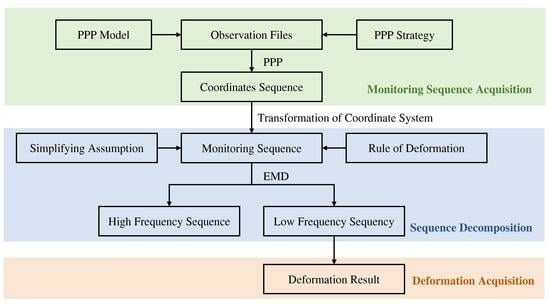
:Although deformations are mostly insignificant, they can be catastrophic when accumulated to certain amounts. Precise point positioning (PPP) can work with one receiver, preventing problems caused by the base station constrain upon employment of current methods such as real-time kinematics (RTK). However, current methods employing PPP focus on high-frequency monitoring such as earthquake or geological calamity monitoring, and these methods are not suitable for structures. Thus, this study proposes a new method for the deformation monitoring of structures via PPP. First, we obtained the coordinate sequence of structures via static PPP when setting the interval. Then, we transformed the coordinates to the same coordinate system with the same basis. Finally, we decomposed the sequences via empirical mode decomposition (EMD) to obtain a low-frequency part, which is the deformation of the target structure. The result of the monitoring experimentation on IGS stations shows that the monitoring index, , of the sequence under different intervals using this method could be 1–2 mm on average in the directions of E, N, and U, which is much better than the original monitoring sequence. Alongside that, it prevented a fall in accuracy when the interval decreased. Therefore, all results proved the feasibility and validity of the method.
1. Introduction
Deformation is inevitable for all human-made structures. The accumulation of deformation to certain values can lead to structural damage. The consequences may cause a significant reduction in the lifespan of the structure or even complete collapse. Nevertheless, modern civil engineering technology has made great progress, which can help minimize the impact of deformation through design or structural reinforcement before failure occurs. However, repairing the structure when deformation surpasses the critical value remains extremely difficult. As such, monitoring the deformation of a target automatically in real time is very necessary for preparations in advance. In recent years, the global navigation satellite system (GNSS) has made significant progress in both theory and practice, and it can fully meet the requirements. Thus, GNSS has been widely applied in deformation monitoring. A typical example is real-time kinematics (RTK) technology [1,2]. RTK can eliminate or weaken the common errors between a rover and a base station, achieving centimeter-level precision in real time [3,4,5,6,7,8]. However, there are also drawbacks. First, the obtained deformation monitoring results represent the relative deformation between the base station and the rover station. Considering the complexity of geological conditions, it cannot be guaranteed that the base station will always remain in its original position or have the same deformation as the rover. Therefore, relative deformation cannot fully reflect the true deformation of the monitoring target. Second, the baseline length between the rover and the base station has limitations in length. The accuracy of the deformation monitoring result is decreased since some errors in positioning cannot be considered equal; on the other hand, the length is increased. Therefore, the base station must not be too far from the rover station [9,10]. Moreover, geological conditions around the rover station cannot always meet the construction requirements of the base station. Hence, existing RTK deformation monitoring methods are not always applicable in practical situations.
Precise point positioning (PPP) is another kind of high-precision positioning technology. It was first proposed by Zumberge in 1997 [11]. PPP can obtain high-precision coordinates under the International Terrestrial Reference Frame (ITRF) by correcting errors in the positioning processes. Moreover, it can achieve millimeter-level accuracy [12,13,14,15,16]. Compared to RTK, PPP can obtain high-precision positioning results without the need for base stations, which means that a single receiver can start working. Additionally, considering that computed coordinates are derived under ITRF, the deformations obtained from these coordinates are absolute deformations, which can fully reflect the real deformation situation compared to relative deformations. These advantages can compensate for the limitations of RTK under unfavorable conditions. Some studies have made progress in using PPP for deformation monitoring [17,18,19,20,21]. Wang et al. monitored the surface subsidence of Houston via PPP [22]. After long-term observations, the accuracy was at the millimeter level. Alcay et al. evaluated the effect of deformation monitoring using PPP through a simulated deformation experiment. The results showed that kinematic PPP could detect 8.1 mm deformation in the horizontal direction and 19.2 mm deformation in the vertical direction; this is close to the effect of relative positioning. Alongside that, the results indicated that the accuracy would worsen with decreased observation time [23], confirming the feasibility of deformation monitoring via PPP. Currently, the applications of PPP in deformation monitoring mostly focus on monitoring geological calamity and earthquakes. Wang et al. used static PPP to monitor the process of slide in their experiment. The results show that the accuracy of PPP can reach 40 mm compared to the results obtained via RTK. Such accuracy is enough for geological calamity monitoring and predictions [24]. Psimoulis et al. calculated the observation data of the global positioning system (GPS) during an earthquake in Japan in 2011 with PPP, concluding that the results of PPP are in accordance with the monitoring data of a seismograph within a certain frequency range [25]. Song et al. proposed a method combining kinematic PPP and static PPP based on sliding window, and the results of a stimulated earthquake experiment indicated that the accuracy of monitoring can achieve 1.5 cm in the horizontal direction and 2.2 cm in the vertical direction [26]. However, challenges still exist when performing practical deformation monitoring of a single target within a small area. The precision of the coordinates obtained via PPP is related to the duration of observation, whereby precision decreases with the decrease in length. This introduces errors in the monitoring sequence, leading to sequence fluctuations and drowning out the real deformation information. Therefore, the key issue relates to how to separate real deformation from the monitoring sequence.
Considering the deformation patterns of structures, structure deformation can be divided into two parts: dynamic deformation and static deformation. In general, most structures have high rigidity, so static deformation dominates the overall deformation, while the dynamic deformation can be neglected. Therefore, we mainly focused on structures that satisfy this condition. In other words, real deformation was approximated as deformation of the static structure in this study. Since changes in static structure deformation are very gradual and small, this process can last several days or weeks. Unlike vibrations, it has an approximately infinitely long periodicity. This could serve as the basis for separating real deformation from the sequence. Empirical mode decomposition (EMD) could decompose a signal into a set of intrinsic mode functions (IMFs) and a residue with an infinitely long period. If EMD is applied to the monitoring sequence of PPP, signals at different frequencies will be decomposed into different IMFs, while the part with infinitely long periodicity will be preserved in the residue of the sequence [27,28,29]. The residue coincides with the real deformation of the target. The real deformation of the target can be successfully separated from the original PPP monitoring sequence.
In summary, this study proposes a new method of deformation monitoring via PPP. Initially, we utilized PPP to obtain coordinates within setting arcs. Through the transformation from global coordinates to local site coordinates, the original sequence is formed. Next, we took advantage of the gap between the frequencies of static deformation and interference data, decomposing the original sequence with EMD. The low-frequency part is the static deformation information which can establish the final deformation monitoring sequence. To validate the feasibility and effectiveness of this method, actual observational data from the International GNSS Service (IGS) terrestrial tracking station network were utilized for deformation monitoring experiments.
2. Materials and Methods
2.1. Original Monitoring Sequence of PPP
2.1.1. Precise Point Positioning
Precise point positioning (PPP) is a typical example of the new generation of high-precision positioning technology. It corrects or estimates errors introduced by various error sources using precise product correction, model correction, and parameter estimation methods, thereby achieving high-accuracy positioning results. This technique simultaneously obtains two types of fundamental observation values for distance measurement, pseudorange observations and carrier phase observations. The basic observation equation for the carrier phase and pseudorange of a satellite at a specific frequency point for a receiver at a specific epoch can be expressed according to the following Formula (1):
In the equation, represents the geometric distance between the satellite and the receiver; denotes the tropospheric delay; signifies the ionospheric delay factor related to frequency; and refers to the ionospheric delay at frequency point 1; is the signal propagation speed; while and are the receiver and satellite clock bias, respectively; and correspond to the wavelength and integer ambiguity at frequency point , respectively; and represent the phase hardware delays at the receiver end and satellite end, respectively; and denote the pseudorange hardware delays at the receiver and satellite, respectively; and indicate the sum of observation noise and multipath errors in the carrier phase and pseudorange observations, respectively.
In the process of PPP, accurate satellite coordinates, satellite clock differences, hardware delays of satellite, antenna phase deviations, and other correcting information can be obtained through various precision products provided by the Satellite Analysis Center. The precise products can diminish the errors introduced by these aspects in positioning. The ionospheric delay, as one of the main sources of error in the positioning process, can be eliminated or reduced by adopting different observation models. The ionosphere-free (IF) combination model is one of the earliest proposed PPP observation models and the most widely applied PPP function model currently. This model uses dual-frequency observations, eliminates the effects of the first-order ionospheric component (accounting for over 90% of the ionospheric delay) through linear combinations, therefore significantly reducing the quantity of parameters to be estimated. The combination of these observed values is represented by Formula (2).
In the equation, and represent the frequencies and , respectively; and are the carrier phase observations for frequencies and ; and and are the pseudorange observations for frequencies and . After rearrangement, IF combination can be expressed by Formula (3).
Apart from the error combination item through the correction of precise products and the correction of the model, the remaining items can be treated as parameters to be estimated together with the target coordinates. The solution is obtained through parameter estimation, finally achieving high-precision positioning results.
2.1.2. Acquiring Monitoring Sequence
Assuming the authentic coordinate sequence of a target within the monitoring time interval is denoted as . The number of observation epochs within interval is represented by and the monitoring coordinate sequence, , is composed of the coordinates obtained at each epoch by PPP. and can be represented by Formula (4).
when the deformation velocity, , approaches zero, considering a tiny arc of which the length is represented by. The slight movement within the time, , can be roughly treated as no deformation. Thus, the authentic coordinates at each time point within are perceived as equal, which can be represented by Formula (5).
We can divide the monitoring time interval, , uniformly into intervals with a length equal to , denoted as . Thus, the authentic coordinate value observed at each moment within the interval, , can be approximated as , where , and it can be noted as , where We assume that there are observation epochs in . When solving with static PPP, this is equivalent to observing a stationary target within over epochs. This means that it is equal to utilizing the Kalman filter for computation under the situation of zero process noise. Thus, the coordinates obtained from epochs within are denoted as , as shown in Formula (6).
According to the process of static PPP, the highest accuracy of coordinates within corresponds to the coordinates obtained from the last epoch. We can assume that the final coordinates of the monitoring arc within are , and therefore, the coordinate monitor sequence can be approximated as , where , as shown in Formula (7); this is the desired monitoring sequence.
2.1.3. Transformation of the Coordinate System
Since the coordinates obtained from PPP in the earth-centered, earth-fixed (ECEF) system are not intuitive enough to describe deformation, we need to convert the coordinates monitoring sequence, , to the East–North–Up (ENU) coordinate system in order to intuitively display the actual deformation monitoring results. We selected the monitoring benchmark in the geodetic coordinate system and obtained the corresponding benchmark coordinates, , in ECEF. The transformation can be represented by Formula (8).
In the formula, is the eccentricity of the reference ellipsoid and is the radius of curvature of the reference ellipsoid at the monitoring target. Their specific values could be found in the parameters of the specific reference ellipsoid. Next, we calculated the position of each coordinate value of in the ENU coordinate system with as the benchmark. It can be represented as Formula (9).
Here, is the transformation matrix and it can be calculated using the location of longitude and latitude of the station. The specific values can be represented by Formula (10).
Similarly, we can convert the true coordinate sequence, , to the ENU coordinate system with as the coordinate origin, denoted as , where .
2.2. Analysis of the Monitoring Sequence
2.2.1. Simplifying Assumption
The deformation sequence of the monitoring target can be regarded as a signal that varies with space and time. Due to error influences, the sequence information includes actual deformation information of the monitoring target, random noise, geoscientific periodic responses, etc. To simplify the problem, we made the following assumptions:
- The precision of the coordinates obtained under the same length of the monitoring arc segment was assumed to be the same and the errors were assumed to be independent and identically distributed among the monitoring coordinate sequence process.
- There are corresponding periods of fluctuation in the monitoring sequence. Random noise is related to the count of monitoring arc segments due to the unique data characteristics. Both parts can be seen as signals at a certain fixed frequency.
- Due to the structure of the project and the requirements of the engineering specifications, the deformation of the construction is inevitably slow. Compared to the periodic fluctuation signals and random errors, we can assume the period of static deformation information to be infinitely long, or a non-frequent signal.
Then, we analyzed the deformation monitoring of the target after making these simplifying assumptions. First, it can be assumed that the monitoring sequence of the monitoring target includes the target’s static deformation, fluctuation disturbance signal, and random noise based on the content of Assumptions 1 and 2. The deformation monitoring sequence, , where , can be represented as the time series , and this time series can be expressed by Formula (11).
In the formula, is the actual deformation state of the target; is the fluctuating disturbance signal of the monitoring sequence; and is the random noise in the monitoring sequence. Moreover, and can be seen as signals at a certain fixed frequency. For the actual static deformation, , the rate of change is very slow according to Assumption 3. Compared to the frequency of fluctuation disturbance signals and random noise, its frequency is very low. Therefore, it is possible to extract from according to the frequency difference between , and . In other words, we need to decompose the synthetic signal and keep the low-frequency items which contain static deformation information in the decomposition results.
2.2.2. Empirical Mode Decomposition
There are currently many signal decomposition methods, such as Fourier transform, wavelet transform, and EMD. Considering that deformation monitoring sequences can be regarded as non-stationary signals, Fourier transform, commonly used for stationary signal processing, is not applicable in this case. Compared to Fourier transform, wavelet transform is applicable for non-stationary signal processing but requires the pre-selection of basic functions and is not entirely adaptive in decomposition. On the other hand, EMD, compared to the aforementioned methods, is not only suitable for non-stationary signal processing, but also achieves fully adaptive signal decomposition. Therefore, in this paper, the EMD method was chosen for signal decomposition.
Empirical mode decomposition (EMD) is a method for analyzing non-stationary signals, first proposed by Huang in 1998 [30]. This algorithm assumes that complex signals can decompose into a finite number of intrinsic mode functions (IMFs). Decomposed IMF components contain the local feature signal components of different time scales in the original signal. In essence, it is a recursive signal decomposition algorithm that identifies the vibration modality of a signal by its time scale. Because it does not require setting any basis functions or prior knowledge in advance, it is theoretically suitable for the decomposition of all signals. Regarding IMF, Huang believes it should satisfy the following conditions:
- The numbers of extremum points and zero-crossing points in the entire signal sequence are the same or differ by one at most;
- The average of the upper and lower envelopes defined by the maximum and minimum values at any time is zero.
According to the definition, the IMF component meets the requirements of a single-signal component and can be seen as an amplitude-modulated wave symmetrical to the time axis. Alongside that, the fluctuations in each period of the adjacent zero-crossing point have only one single frequency, without the superimposed signals of other frequencies. Therefore, EMD can decompose signal into a combination of a group of single-frequency signals and a residual with an infinite period; that is to say, any signal after EMD treatment can be expressed by Formula (12):
The specific process of EMD can be outlined as follows:
- Find all the maximum and minimum values in signal . Fit the maximum and minimum values, respectively, to obtain the upper and lower envelope lines in signal with the cubic spline curve.
- Calculate the average at each point of the upper and lower envelopes and obtain the average line, denoted as .
- Calculate and check whether conforms to the IMF component definition. If not, treat as the new , and redo Steps 1, 2 and 3 until meets the IMF component definition or the set screening threshold, denoted as .
- Recast as signal , and reiterate Steps 1, 2, 3, 4 until no new IMF component can be separated from signal . The remaining part is recorded as .
The complete flow chart following this reorganization is displayed in Figure 1.
2.3. Experimentation
2.3.1. Data Resource
The International GNSS Service (IGS), formerly known as the International GPS Service Organization, primarily serves to provide accurate standard data and products for GNSS, facilitating earth science research, interdisciplinary applications, and education. To this end, IGS has established a multitude of GNSS monitoring stations, forming a global ground-tracking station network. Currently, the number of monitoring stations operating under IGS worldwide exceeds 500.
The station structure, which is vertically short but horizontally expansive, is constructed using reinforced concrete, resulting in substantial bending stiffness, as shown in Figure 2. Therefore, their responses to dynamic loads, such as vibrations, are minimal, with dynamic deformations typically approximated as negligible. Additionally, the structures are surrounded by stainless steel barrels which mitigate the impact of thermal deformation due to temperature fluctuations. Consequently, it is evident that there are no other deformations in the IGS station except for static deformation. Alongside this, all observational data collected by the global ground-tracking stations network of the GNSS are gathered, archived, and distributed by the IGS to the global network. This allows any user to access relevant observational data and products through the IGS network interface. Considering these factors—the deformation characteristics of IGS stations aiding in the elimination of the potential experimental interference and the comprehensive, easily accessible observational data—selecting IGS station observational data for actual deformation monitoring experiments is a logical choice. For this experimentation, eleven IGS stations were chosen, the specific distribution of which is described in Figure 3.
2.3.2. Configuration and Strategy
The observation data were selected from the observation files provided by the IGS with a sampling frequency of 30 s. The experimental period was set for 49 days, from 6 February 2022 to 26 March 2022. The reference coordinate series for the stations were derived from the coordinates given by the weekly SINEX files provided by the IGS using linear interpolation. In this experiment, the benchmark coordinates for each station were calculated using the coordinates provided by the weekly SINEX files from 5 February 2022. Since the positioning accuracy of static PPP is influenced by the number of its observation epochs, the longer the observation time is after convergence under equivalent observation conditions, the higher the static PPP positioning accuracy is. Therefore, we considered setting different observation arc lengths and comparing the monitoring effect of the monitoring series under different monitoring arc lengths in this experiment. That is to say, we took different values for interval . Considering the convergence time of static PPP, the final observation arc lengths were set to 24 h, 12 h, 8 h, 6 h, 4 h, 3 h, and 2 h, respectively.
Regarding the PPP strategy, we made the following choices in this experiment. The satellite system used was single-GPS system. The ionosphere-free combination observation model as adopted to eliminate ionospheric delay. The final orbit product and clock difference product provided by the IGS were used to correct satellite orbit error and satellite clock difference, respectively. Forward Kalman filtering was used to estimate parameters such as receiver coordinates, tropospheric delay wet component, and receiver clock difference. The specific solution process of precise point positioning used the multi-frequency multi-mode GNSS solution software MUSIP (version 1.0) developed by the Tongji GNSS team of Tongji University [10,31]. The complete PPP data processing strategy is shown in Table 1.
3. Results
After the PPP calculation for different lengths of monitoring time, the corresponding coordinate values were obtained utilizing the observational data from each IGS ground tracking station. The resultant original PPP monitoring sequences were obtained, as depicted in Figure 4, after the conversion of the coordinate system. It should be noted that there, the typical result of one station CEDU is also shown in Figure 4 and the results of the other stations in experimentation are shown in Figure A1. Intuitively, the monitoring sequences obtained from different tracking arcs fluctuate around the reference sequence or show a constant deviation of the latter from the graphical representation of the monitoring results. Moreover, it can be visually observed that the deformation monitoring sequences, derived from various lengths of monitoring arc segments, exhibit apparent periodical fluctuations as the monitoring arcs reduce. The ranged fluctuations become wider and more complex as the arcs continue to shorten. When it shrinks to 6 h, the monitoring sequence, due to its excessive wave range and overly complicated wave format, cannot reliably reflect the target’s static deformation.
Next, the sequences were decomposed using EMD to obtain the residual as the extracted static deformation of the IGS ground tracking station. The static deformation monitoring sequence results are shown in Figure 5. As in Figure 4, the typical results of station CEDU and the results of the other stations in experiment are shown in Figure A2. Intuitively, the extracted static deformation sequence after EMD decomposition clearly eliminates the wave phenomenon compared to the original PPP deformation monitoring sequence. Furthermore, the PPP deformation monitoring sequence shows a high similarity to the sequence formed by the reference coordinates provided in the SINEX file, with the best fit in the N direction, followed by the E direction, and the worst fit in the U direction.
4. Discussion
4.1. Monitoring Index Sd
The evaluation of the monitoring effect of the deformation monitoring sequence can be understood as evaluating the distribution of errors within the monitoring sequence. The relationship between the deformation monitoring sequence, , and the true deformation sequence, , are represented by Formula (13).
In the above formula, is obtained from via the transformation matrix . According to previous assumptions, it is logical to hypothesize that the error of the positioning results obtained from static PPP under the same observation duration, , is independent and identically distributed (iid) in the same direction, . Given that the transformation matrix, , is a linear transformation, the errors in the same direction, , still maintain the same probability density function and remain independent after the transformation. Consequently, as shown in Formula (14), has identical expectation and variance.
Because is iid, it can be considered that random experiments have been conducted on the random variable . Therefore, standard deviation can be used to describe the random variable , as shown in Formula (15).
reflects the distribution of the error in direction . Thus, it can be used as an index to evaluate the monitoring effect. In summary, we took the standard deviation of the sequence difference between the deformation monitoring sequence and the deformation reference sequence as an evaluation metric for static deformation monitoring effectiveness.
4.2. Analysis of the Monitoring Result
4.2.1. Original Monitoring Sequence of PPP
To further evaluate the monitoring effect of different-length arcs, the values of all monitoring arcs are calculated statistically and averaged. The result of it is displayed in Table 2. As observed from the table, the monitoring arc of 24 h allows for the best PPP performance, with an average value of 4.81 mm, 3.86 mm, and 9.87 mm in the E, N, and U directions, respectively. In contrast, the worst monitoring effect is found within the 2 h arc, where the values reached 34.96 mm, 12.05 mm, and 38.92 mm in the E, N, and U directions, respectively. In the same direction, the values differed substantially across different-length arcs and this disparity remained large in the same monitoring length across different directions. The average statistics on values were paired with the graphical mapping of the monitoring sequence, verifying the following conclusions:
- Static deformation information is present in the original PPP deformation monitoring sequence.
- The static deformation information in the original PPP deformation monitoring sequence is drowned out by the fluctuations.
- As the monitoring arc shortens, the fluctuations in the original PPP deformation monitoring sequence become more pronounced, exacerbating the drowning out effect of static deformation information.
4.2.2. Extracting the Monitoring Sequence of PPP
Similarly, the values of all monitoring arcs were statistically analyzed and their average values obtained to further evaluate and compare the PPP deformation monitoring effects under different monitoring arcs, as shown in Table 3. From the table, it can be seen that the 24 h monitoring arc has the best PPP deformation monitoring effect, with values of 1.09 mm, 1.74 mm, and 1.88 mm in the E, N, and U directions, respectively, while the 2 h monitoring arc has the worst PPP deformation monitoring effect, with values of 2.81 mm, 1.71 mm, and 3.37 mm in E, N, and U directions, respectively. Overall, as the monitoring arc shortens, increases and the monitoring effect of the PPP deformation sequence deteriorates. This is similar to the results of the original PPP deformation monitoring sequence. However, the difference is that there is no significant change in the results between arcs of the same direction but different lengths, or between arcs of different directions but the same length, as observed in the original PPP deformation monitoring sequence. Combining the results obtained from the original PPP deformation monitoring sequence, it can be concluded that after the target static deformation is extracted via EMD decomposition, the interference information or wave signals in the PPP deformation monitoring sequence are effectively eliminated, and the extracted target static deformation has a small error compared to the actual static deformation. Furthermore, it effectively prevents a significant decrease in the PPP deformation monitoring effect caused by the shortening of the monitoring arc. Thus, it verified the feasibility and effectiveness of the deformation monitoring method proposed in this paper.
5. Conclusions
We proposed a new method for static deformation monitoring in this paper. First, we analyzed the principles and methods of obtaining the deformation monitoring of the target using PPP technology while considering the slow deformation rate and the minute deformation of the target static deformation. Then, we used EMD algorithm to decompose the static deformation information which was submerged in the fluctuation signal of the original PPP deformation monitoring sequence. Finally, we obtained the static deformation information of the low-frequency term from the PPP deformation monitoring sequences. In order to verify the reliability of this method, PPP deformation monitoring experiments were conducted using IGS ground tracking station observational data where static deformation dominated. By analyzing the original PPP deformation monitoring sequence in the experiment, it was found that the original PPP deformation sequence always fluctuates significantly around the reference sequence, which further verifies that the original PPP deformation monitoring sequence contains the target’s static deformation information. However, static information is also submerged by fluctuation signals, making it impossible to exhibit intuitively at the same time. Additionally, the value of the monitoring sequences continued increasing as the monitoring arc shortened and the submergence phenomenon becomes more serious. Compared to the original PPP deformation monitoring sequence, the extracted PPP deformation monitoring sequence after EMD was very close to the reference value sequence, and the fluctuation phenomenon was eliminated, indicating its monitoring effectiveness. From the changes in the value and the sequence diagram, it can be seen that the monitoring effect of the extracted PPP deformation monitoring sequence did not change dramatically with the shortening of the monitoring arc, indicating the stability of its monitoring effect.
Therefore, the effectiveness and stability of deformation monitoring demonstrated by this method jointly indicate the feasibility and effectiveness of this method. However, in this study, only low-frequency term information of the EMD decomposition result was taken, but the high-frequency term information in each IMF was not fully utilized, and the EMD algorithm decomposition result was affected by the endpoint effect and modal aliasing phenomenon, which adversely affects the decomposition result. Future research should consider the actual physical meaning of each IMF and adopt improved EMD algorithms to prevent or weaken the impact of endpoint effects and modal aliasing phenomena on the extraction results.
Author Contributions
R.L. was responsible for designing the experiment, writing code, writing the original manuscript, and analyzing the results of experiment. H.G. and Z.Z. were responsible for the revision of this article and providing the overall conception of this research. Y.G. and J.Z. were responsible for the data attainment and discussion of the results. All authors have read and agreed to the published version of the manuscript.
Funding
This research was funded by the Natural Science Funds of Shanghai, grant number 21ZR1465600.
Data Availability Statement
The original data files in the monitoring experimentation were obtained from the observation files from the IGS (https://igs.org (accessed on 1 October 2023)).
Acknowledgments
The authors would like to thank the Fundamental Research Funds for the Central Universities and Natural Science Funds of Shanghai (21ZR1465600).
Conflicts of Interest
The authors declare no conflict of interest.
Appendix A
Figure A1.
(a) Original monitoring sequence of ALIC; (b) original monitoring sequence of DARW; (c) original monitoring sequence of KAT1; (d) original monitoring sequence of MCHL; (e) original monitoring sequence of MOBS; (f) original monitoring sequence of NNOR; (g) original monitoring sequence of PARK; (h) original monitoring sequence of SYDN; (i) original monitoring sequence of TOW2; (j) original monitoring sequence of YAR2.


Figure A2.
(a) Extracted monitoring sequence of station ALIC; (b) extracted monitoring sequence of station DARW; (c) extracted monitoring sequence of station KAT1; (d) extracted monitoring sequence of station MCHL; (e) extracted monitoring sequence of station MOBS; (f) extracted monitoring sequence of station NNOR; (g) extracted monitoring sequence of station PARK; (h) extracted monitoring sequence of station SYDN; (i) extracted monitoring sequence of station TOW2; (j) extracted monitoring sequence of station YAR2.


References
- Du, Y.; Huang, G.; Zhang, Q.; Gao, Y.; Gao, Y. Asynchronous RTK Method for Detecting the Stability of the Reference Station in GNSS Deformation Monitoring. Sensors 2020, 20, 1320. [Google Scholar] [CrossRef] [PubMed]
- Nadarajah, N.; Khodabandeh, A.; Wang, K.; Choudhury, M.; Teunissen, P. Multi-GNSS PPP-RTK: From Large- to Small-Scale Networks. Sensors 2018, 18, 1078. [Google Scholar] [CrossRef]
- Gao, J.; Liu, C.; Wang, J.; Li, Z.; Meng, X. A New Method for Mining Deformation Monitoring with GPS-RTK. Trans. Nonferrous Met. Soc. China 2011, 21, S659–S664. [Google Scholar] [CrossRef]
- Zhao, L.; Yang, Y.; Xiang, Z.; Zhang, S.; Li, X.; Wang, X.; Ma, X.; Hu, C.; Pan, J.; Zhou, Y.; et al. A Novel Low-Cost GNSS Solution for the Real-Time Deformation Monitoring of Cable Saddle Pushing: A Case Study of Guojiatuo Suspension Bridge. Remote Sens. 2022, 14, 5174. [Google Scholar] [CrossRef]
- Xi, R.; Jiang, W.; Meng, X.; Chen, H.; Chen, Q. Bridge Monitoring Using BDS-RTK and GPS-RTK Techniques. Measurement 2018, 120, 128–139. [Google Scholar] [CrossRef]
- Luo, L.; Ma, W.; Zhang, Z.; Zhuang, Y.; Zhang, Y.; Yang, J.; Cao, X.; Liang, S.; Mu, Y. Freeze/Thaw-Induced Deformation Monitoring and Assessment of the Slope in Permafrost Based on Terrestrial Laser Scanner and GNSS. Remote Sens. 2017, 9, 198. [Google Scholar] [CrossRef]
- Jing, C.; Huang, G.; Zhang, Q.; Li, X.; Bai, Z.; Du, Y. GNSS/Accelerometer Adaptive Coupled Landslide Deformation Monitoring Technology. Remote Sens. 2022, 14, 3537. [Google Scholar] [CrossRef]
- Chen, Q.; Jiang, W.; Meng, X.; Jiang, P.; Wang, K.; Xie, Y.; Ye, J. Vertical Deformation Monitoring of the Suspension Bridge Tower Using GNSS: A Case Study of the Forth Road Bridge in the UK. Remote Sens. 2018, 10, 364. [Google Scholar] [CrossRef]
- Chen, D.; Ye, S.; Xia, F.; Cheng, X.; Zhang, H.; Jiang, W. A Multipath Mitigation Method in Long-Range RTK for Deformation Monitoring. GPS Solut. 2022, 26, 1–12. [Google Scholar] [CrossRef]
- Li, B.; Shen, Y.; Feng, Y.; Gao, W.; Yang, L. GNSS Ambiguity Resolution with Controllable Failure Rate for Long Baseline Network RTK. J. Geod. 2014, 88, 99–112. [Google Scholar] [CrossRef]
- Zumberge, J.; Heflin, M.; Jefferson, D.; Watkins, M.; Webb, F. Precise Point Positioning for the Efficient and Robust Analysis of GPS Data from Large Networks. J. Geophys. Res. Solid Earth 1997, 102, 5005–5017. [Google Scholar] [CrossRef]
- Zheng, Y.; Zhang, R.; Gu, S. A New PPP Algorithm for Deformation Monitoring with Single-Frequency Receiver. J. Earth Syst. Sci. 2014, 123, 1919–1926. [Google Scholar] [CrossRef]
- Xiao, G.; Li, P.; Gao, Y.; Heck, B. A Unified Model for Multi-Frequency PPP Ambiguity Resolution and Test Results with Galileo and BeiDou Triple-Frequency Observations. Remote Sens. 2019, 11, 116. [Google Scholar] [CrossRef]
- Li, X.; Li, X.; Ma, F.; Yuan, Y.; Zhang, K.; Zhou, F.; Zhang, X. Improved PPP Ambiguity Resolution with the Assistance of Multiple LEO Constellations and Signals. Remote Sens. 2019, 11, 408. [Google Scholar] [CrossRef]
- Katsigianni, G.; Loyer, S.; Perosanz, F. PPP and PPP-AR Kinematic Post-Processed Performance of GPS-Only, Galileo-Only and Multi-GNSS. Remote Sens. 2019, 11, 2477. [Google Scholar] [CrossRef]
- Bertiger, W.; Desai, S.; Haines, B.; Harvey, N.; Moore, A.; Owen, S.; Weiss, J. Single Receiver Phase Ambiguity Resolution with GPS Data. J. Geod. 2010, 84, 327–337. [Google Scholar] [CrossRef]
- Yang, H.; Ji, S.; Weng, D.; Wang, Z.; He, K.; Chen, W. Assessment of the Feasibility of PPP-B2b Service for Real-Time Coseismic Displacement Retrieval. Remote Sens. 2021, 13, 5011. [Google Scholar] [CrossRef]
- Gao, R.; Liu, Z.; Odolinski, R.; Jing, Q.; Zhang, J.; Zhang, H.; Zhang, B. Hong Kong-Zhuhai-Macao Bridge Deformation Monitoring Using PPP-RTK with Multipath Correction Method. GPS Solut. 2023, 27, 195. [Google Scholar] [CrossRef]
- Araszkiewicz, A. Integration of Distributed Dense Polish GNSS Data for Monitoring the Low Deformation Rates of Earth’s Crust. Remote Sens. 2023, 15, 1504. [Google Scholar] [CrossRef]
- Zang, N.; Li, B.; Nie, L.; Shen, Y. Inter-System and Inter-Frequency Code Biases: Simultaneous Estimation, Daily Stability and Applications in Multi-GNSS Single-Frequency Precise Point Positioning. GPS Solut. 2019, 24, 18. [Google Scholar] [CrossRef]
- Zheng, K.; Zhang, X.; Li, X.; Li, P.; Chang, X.; Sang, J.; Ge, M.; Schuh, H. Mitigation of Unmodeled Error to Improve the Accuracy of Multi-GNSS PPP for Crustal Deformation Monitoring. Remote Sens. 2019, 11, 2232. [Google Scholar] [CrossRef]
- Wang, G.; Turco, M.; Soler, T.; Kearns, T.; Welch, J. Comparisons of OPUS and PPP Solutions for Subsidence Monitoring in the Greater Houston Area. J. Surv. Eng. 2017, 143, 05017005. [Google Scholar] [CrossRef]
- Alcay, S.; Ogutcu, S.; Kalayci, I.; Yigit, C. Displacement Monitoring Performance of Relative Positioning and Precise Point Positioning (PPP) Methods Using Simulation Apparatus. Adv. Space Res. 2019, 63, 1697–1707. [Google Scholar] [CrossRef]
- Wang, L.; Zhang, X.; Huang, G.W.; Tu, R.; Zhang, S.C. Experiment Results and Analysis of Landslide Monitoring by Using GPS PPP Technology. Rock Soil Mech. 2014, 35, 2118–2124. [Google Scholar]
- Psimoulis, P.; Houlié, N.; Meindl, M.; Rothacher, M. Consistency of PPP GPS and Strong-Motion Records: Case Study of Mw9.0 Tohoku-Oki 2011 Earthquake. Smart Struct. Syst. 2015, 16, 347–366. [Google Scholar] [CrossRef]
- Song, W.; Zhang, R.; Yao, Y.; Liu, Y.; Hu, Y. PPP Sliding Window Algorithm and Its Application in Deformation Monitoring. Sci. Rep. 2016, 6, 26497. [Google Scholar] [CrossRef] [PubMed]
- Boudraa, A.; Cexus, J. EMD-Based Signal Filtering. IEEE Trans. Instrum. Meas. 2007, 56, 2196–2202. [Google Scholar] [CrossRef]
- Niu, Y.; Xiong, C. Analysis of the Dynamic Characteristics of a Suspension Bridge Based on RTK-GNSS Measurement Combining EEMD and a Wavelet Packet Technique. Meas. Sci. Technol. 2018, 29, 085103. [Google Scholar] [CrossRef]
- Wang, T.; Zhang, M.; Yu, Q.; Zhang, H. Comparing the Applications of EMD and EEMD on Time-Frequency Analysis of Seismic Signal. J. Appl. Geophys. 2012, 83, 29–34. [Google Scholar] [CrossRef]
- Huang, N.; Shen, Z.; Long, S.; Wu, M.; Shih, H.; Zheng, Q.; Yen, N.; Tung, C.; Liu, H. The Empirical Mode Decomposition and the Hilbert Spectrum for Nonlinear and Non-Stationary Time Series Analysis. Proc. R. Soc. Math. Phys. Eng. Sci. 1998, 454, 903–995. [Google Scholar] [CrossRef]
- Li, B.; Zhang, Z.; Zang, N.; Wang, S. High-Precision GNSS Ocean Positioning with BeiDou Short-Message Communication. J. Geod. 2019, 93, 125–139. [Google Scholar] [CrossRef]
Figure 1.
Complete process of the EMD algorithm.

Figure 2.
Station setting of the global network of the IGS ground tracking stations: (a) setting of station KAT1; (b) setting of station KAT1.
Figure 2.
Station setting of the global network of the IGS ground tracking stations: (a) setting of station KAT1; (b) setting of station KAT1.

Figure 3.
Location of IGS ground tracking stations in this experiment.

Figure 4.
Original monitoring sequence of PPP under different lengths of duration.

Figure 5.
Extracting the monitoring sequence of PPP under different lengths of duration.


Table 1.
PPP strategy in this experimentation.
| Item | Strategy |
|---|---|
| Satellite orbit | IGS final precise orbit product-sp3 |
| Satellite clock | IGS final precise clock product-clk |
| Antenna bias | IGS18.atx |
| Ionospheric delay | Ionosphere-free combination |
| Ambiguity | Float resolution |
| Receiver coordinate | Parameter estimation |
| Receiver clock | Parameter estimation |
| Tropospheric delay | ZTD estimation |
| Solid tide correction | Spherical harmonic function correction |
Table 2.
Average in the original monitoring sequence of PPP with different lengths of time.
| Item | Direction | East/mm | North/mm | Up/mm |
|---|---|---|---|---|
| Duration | 24 h | 4.82 | 3.86 | 9.87 |
| 12 h | 7.76 | 4.86 | 13.82 | |
| 08 h | 9.96 | 5.44 | 16.16 | |
| 06 h | 11.73 | 6.01 | 18.31 | |
| 04 h | 16.11 | 6.96 | 22.35 | |
| 03 h | 21.10 | 8.48 | 27.66 | |
| 02 h | 34.96 | 12.05 | 38.92 |
Table 3.
Average in extracting the monitoring sequence of PPP with different lengths of time.
| Item | Direction | East/mm | North/mm | Up/mm |
|---|---|---|---|---|
| Duration | 24 h | 1.09 | 1.74 | 1.88 |
| 12 h | 1.18 | 1.55 | 2.25 | |
| 08 h | 1.63 | 1.42 | 2.20 | |
| 06 h | 1.41 | 1.40 | 2.35 | |
| 04 h | 1.52 | 1.40 | 2.49 | |
| 03 h | 1.47 | 1.46 | 2.47 | |
| 02 h | 2.81 | 1.71 | 3.37 |
Disclaimer/Publisher’s Note: The statements, opinions and data contained in all publications are solely those of the individual author(s) and contributor(s) and not of MDPI and/or the editor(s). MDPI and/or the editor(s) disclaim responsibility for any injury to people or property resulting from any ideas, methods, instructions or products referred to in the content. |
© 2023 by the authors. Licensee MDPI, Basel, Switzerland. This article is an open access article distributed under the terms and conditions of the Creative Commons Attribution (CC BY) license (https://creativecommons.org/licenses/by/4.0/).
Share and Cite
MDPI and ACS Style
Li, R.; Zhang, Z.; Gao, Y.; Zhang, J.; Ge, H. A New Method for Deformation Monitoring of Structures by Precise Point Positioning. Remote Sens. 2023, 15, 5743. https://doi.org/10.3390/rs15245743
AMA Style
Li R, Zhang Z, Gao Y, Zhang J, Ge H. A New Method for Deformation Monitoring of Structures by Precise Point Positioning. Remote Sensing. 2023; 15(24):5743. https://doi.org/10.3390/rs15245743
Chicago/Turabian StyleLi, Ruihui, Zijian Zhang, Yu Gao, Junyi Zhang, and Haibo Ge. 2023. "A New Method for Deformation Monitoring of Structures by Precise Point Positioning" Remote Sensing 15, no. 24: 5743. https://doi.org/10.3390/rs15245743
Note that from the first issue of 2016, this journal uses article numbers instead of page numbers. See further details here.