
Mid-Term Monitoring of Suspended Sediment Plumes of Greek Rivers Using Moderate Resolution Imaging Spectroradiometer (MODIS) Imagery


Abstract
:1. Introduction
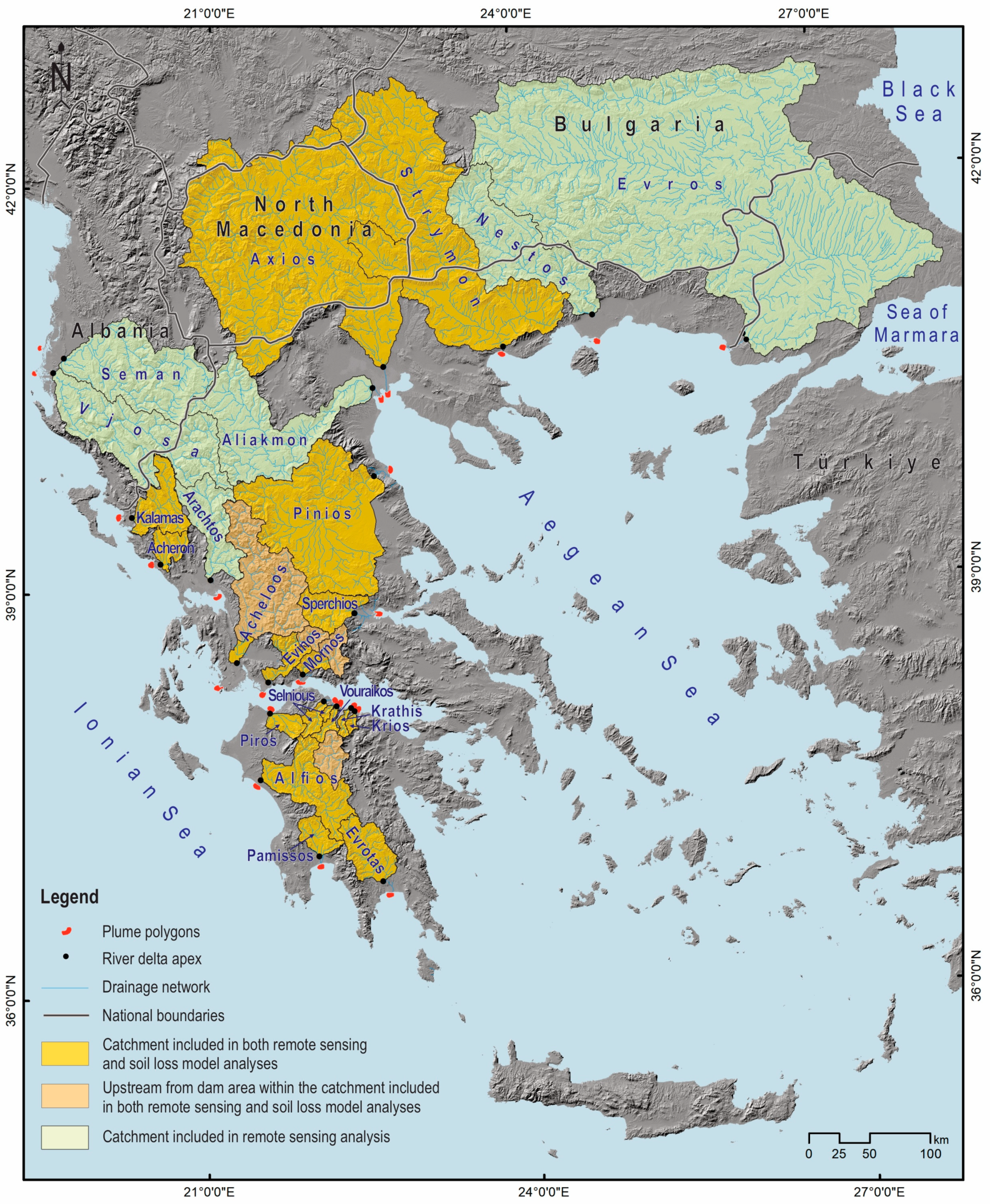
2. Study Area
3. Materials and Methods
3.1. Moderate Resolution Imaging Spectroradiometer (MODIS) Imagery
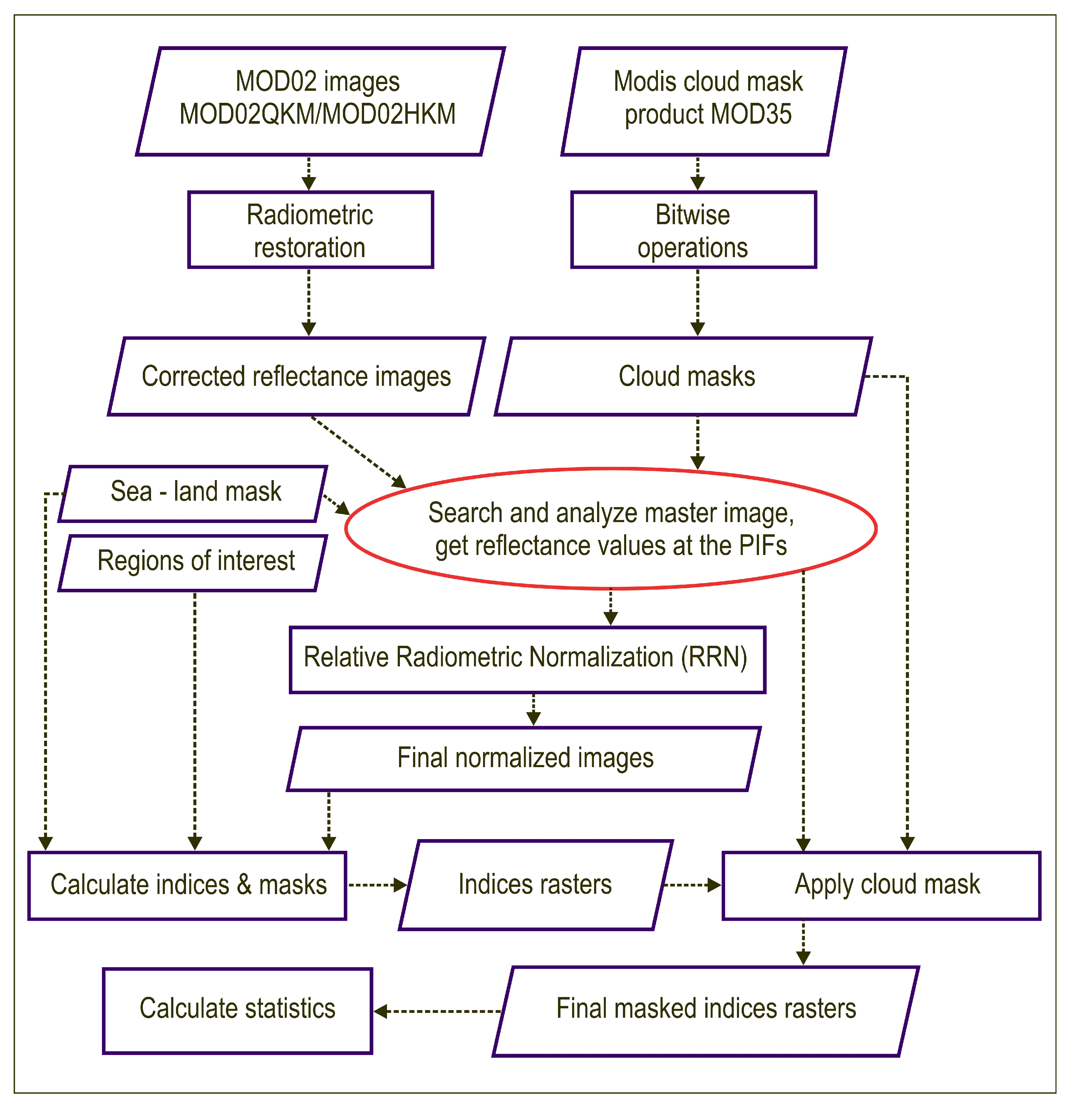
3.1.1. Selection, Acquisition, and Processing of Images
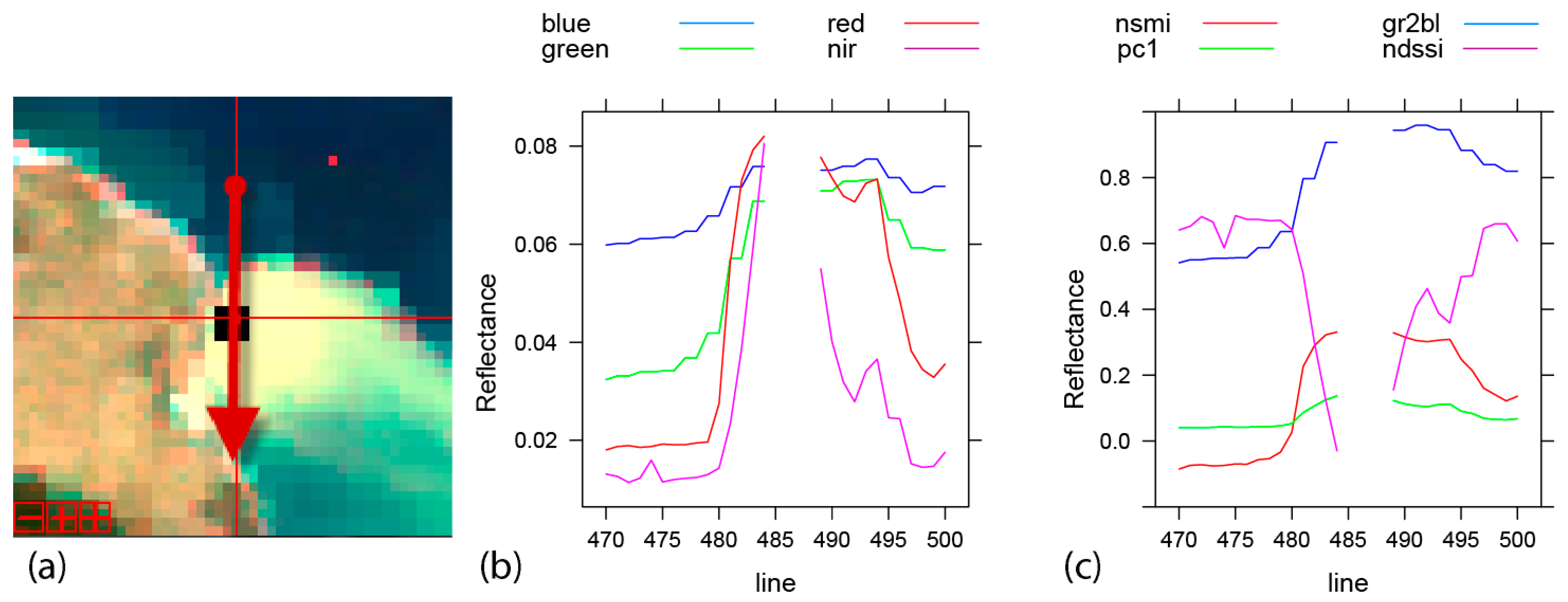
3.1.2. Suspended Sediment/Suspended Material Indices, Ratios and Masks
3.1.3. Soil Loss Models
4. Results and Discussion
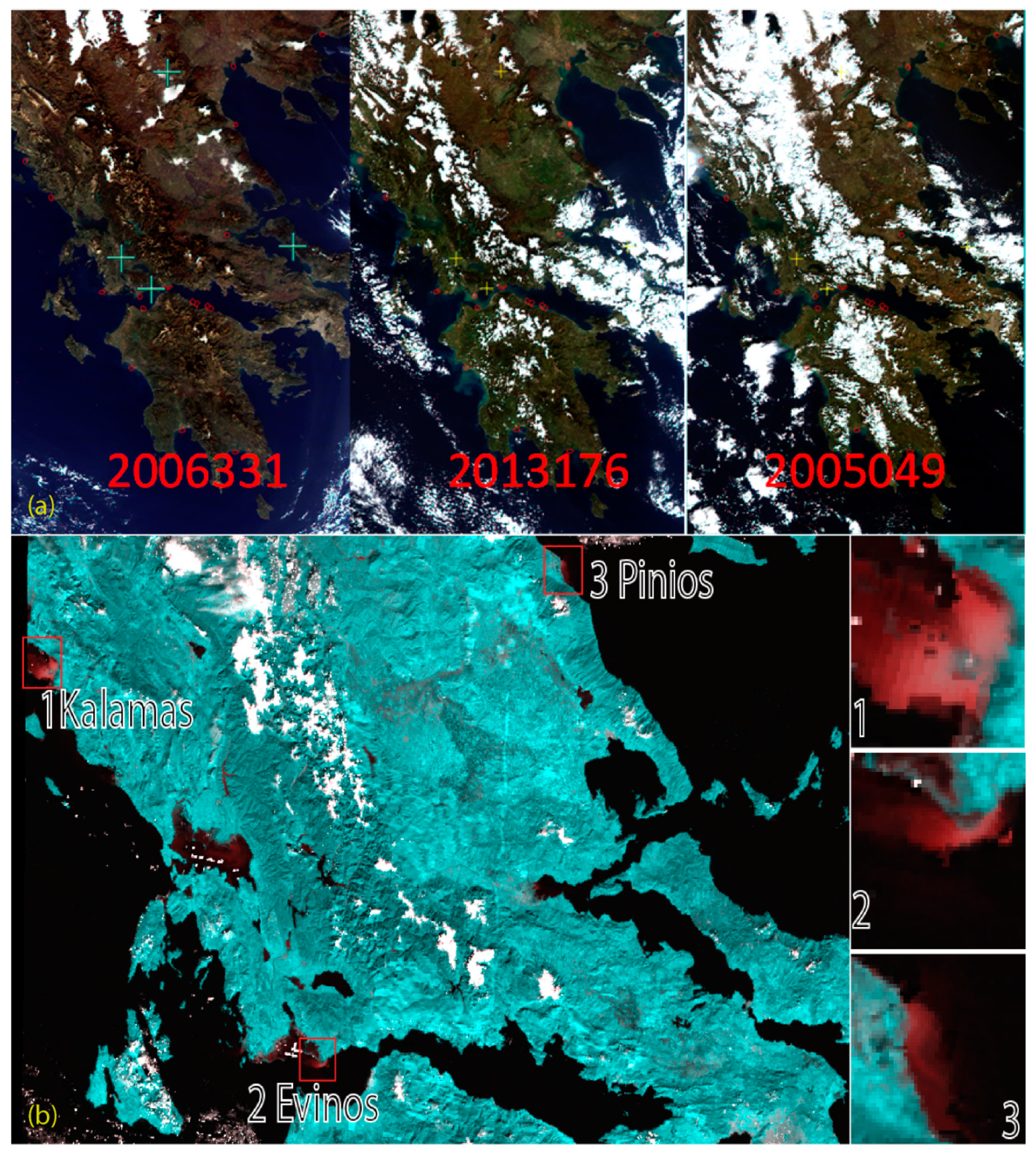
4.1. Moderate Resolution Imaging Spectroradiometer (MODIS) Imagery
4.2. Comparison with Soil Loss Models
5. Conclusions
Author Contributions
Funding
Data Availability Statement
Acknowledgments
Conflicts of Interest
References
- Gregory, K.J.; Walling, D.E. Drainage Basin. Form and Process: A Geomorphological Approach; Edward Arnold: London, UK, 1973; p. 456. [Google Scholar]
- Reid, I.; Bathurst, J.C.; Carling, P.A.; Walling, D.E.; Webb, B.W. Sediment erosion, transport and deposition. In Applied Fluvial Geomorphology for River Engineering and Management; Thorne, C.R., Hey, R.D., Newson, M.D., Eds.; John Wiley & Sons: Chichester, West Sussex, UK, 1997; pp. 95–135. [Google Scholar]
- Turowski, J.M.; Rickenmann, D.; Dadson, S.J. The partitioning of the total sediment load of a river into suspended load and bedload: A review of empirical data. Sedimentology 2010, 57, 1126–1146. [Google Scholar] [CrossRef]
- Anderson, R.; Anderson, S. Geomorphology, the Mechanics and Chemistry of Landscapes; Cambridge University Press: Cambridge, UK, 2010; p. 637. [Google Scholar] [CrossRef]
- Walling, D.E.; Webb, B.W. Erosion and Sediment yield: A global overview. In Proceedings of the Symposium Erosion and Sediment Yield: Global and Regional Perspectives, Exeter, UK, 15–19 July 1996; IAHS Publisher: Hamilton, ON, Canada, 1996; p. 236. [Google Scholar]
- Bourgoin, L.M.; Bonnet, M.P.; Martinez, J.M.; Kosuth, P.; Cochonneau, G.; Moreira-Turcq, P.; Guyot, J.L.; Vauchel, P.; Filizola, N.; Seyler, P. Temporal dynamics of water and sediment exchanges between the Curuaí floodplain and the Amazon River, Brazil. J. Hydrol. 2007, 335, 140–156. [Google Scholar] [CrossRef]
- Filizola, N.; Guyot, J.L. Suspended sediment yields in the Amazon basin: An assessment using the Brazilian national data set. Hydrol. Process. 2009, 23, 3207–3215. [Google Scholar] [CrossRef]
- Sarker, S. Separation of Floodplain Flow and Bankfull Discharge: Application of 1D Momentum Equation Solver and MIKE 21C. CivilEng 2023, 4, 933–948. [Google Scholar] [CrossRef]
- Burgan, H.I. The short-term and seasonal trend detection of sediment discharges in Turkish Rivers. Rocz. Ochr. Środowiska 2022, 24, 214–230. [Google Scholar] [CrossRef]
- Bouchez, J.; Gaillardet, J.; France-Lanord, C.; Maurice, L.; Dutra-Maia, P. Grain size control of river suspended sediment geochemistry: Clues from Amazon River depth profiles. Geochem. Geophys. Geosyst. 2011, 12, Q03008. [Google Scholar] [CrossRef]
- Charlton, R. Fundamentals of Fluvial Geomorphology, 1st ed.; Routledge: London, UK, 2007; p. 264. [Google Scholar]
- Shen, F.; Verhoef, W.; Zhou, Y.; Salama, S.; Liu, X. Satellite Estimates of Wide-Range Suspended Sediment Concentrations in Changjiang (Yangtze) Estuary Using MERIS Data. Estuaries Coasts 2010, 33, 1420–1429. [Google Scholar] [CrossRef]
- Sarker, S.; Sarker, T.; Leta, O.T.; Raihan, S.U.; Khan, I.; Ahmed, N. Understanding the Planform Complexity and Morphodynamic Properties of Brahmaputra River in Bangladesh: Protection and Exploitation of Riparian Areas. Water 2023, 15, 1384. [Google Scholar] [CrossRef]
- Chakrapani, G.J. Factors controlling variations in river sediment loads. Curr. Sci. 2005, 88, 569–575. [Google Scholar]
- Latrubesse, E.M.; Stevaux, J.C.; Sinha, R. Tropical rivers. Geomorphology 2005, 70, 187–206. [Google Scholar] [CrossRef]
- Milliman, J.D.; Farnsworth, K.L.; Jones, P.D.; Xu, K.H.; Smith, L.C. Climatic and anthropogenic factors affecting river discharge to the global ocean, 1951–2000. Glob. Planet. Chang. 2008, 62, 187–194. [Google Scholar] [CrossRef]
- Marinho, R.R.; Filizola, N.P.; Martinez, J.M.; Harmel, T. Suspended sediment transport estimation in Negro River (Amazon Basin) using MSI/Sentinel-2 data. Rev. Bras. Geomorfol. 2022, 23, 1174–1190. [Google Scholar] [CrossRef]
- Pacific Southwest Inter Agency Committee (PSIAC). Factors Affecting Sediment Yield in the Pacific Southwest Area and Selection and Evaluation of Measures for Reduction of Erosion and Sediment Yield; Water Management Subcommitte on American Society of Civil Engineers (ASCE): Reston, VI, USA, 1968; Report No. HY 12. [Google Scholar]
- Wischmeier, W.H.; Smith, D.D. Prediction Rainfall Erosion Losses from Cropland East of the Rocky Mountains: A Guide for Selection of Practices for Soil and Water Conservation. Agric. Handb. 1965, 282, 47. [Google Scholar]
- Wischmeier, W.H.; Smith, D.D. Predicting Rainfall Erosion Losses: A Guide to Conservation Planning; United States Department of Agriculture (USDA), Agricultural Research Service Handbook No. 537; United States Government Printing Office: Washington, DC, USA, 1978; p. 58.
- Renard, K.; Foster, G.; Weesies, G.; McCool, D.; Yoder, D. Predicting Soil Erosion by Water: A Guide to Conservation Planning with the Revised Universal Soil Loss Equation (RUSLE); United States Department of Agriculture, Agricultural Research Service, Agriculture Handbook No. 703; United States Department of Agriculture: Washington, DC, USA, 1997; p. 407.
- Panagos, P.; Borrelli, P.; Poesen, J.; Ballabio, C.; Lugato, E.; Meusburger, K.; Montanarella, L.; Alewell, C. The new assessment of soil loss by water erosion in Europe. Environ. Sci. Pol. 2015, 54, 438–447. [Google Scholar] [CrossRef]
- Milliman, J.D.; Meade, R.H. World-wide delivery of river sediment to the oceans. J. Geol. 1983, 91, 1–21. [Google Scholar] [CrossRef]
- Milliman, J.D.; Syvitski, P.M. Geomorphic/tectonic control of sediment discharge to the ocean: The importance of small mountainous rivers. J. Geol. 1992, 100, 525–544. [Google Scholar] [CrossRef]
- Hovius, N. Controls on sediment supply by large rivers. SEPM Spec. Publ. Soc. Sediment. Geol. 1998, 59, 3–16. [Google Scholar]
- Ludwig, W.; Probst, J.-L. River sediment discharge to the oceans: Present-day controls and global budgets. Am. J. Sci. 1998, 298, 265–295. [Google Scholar] [CrossRef]
- Beusen, A.H.W.; Dekkers, A.L.M.; Bouwman, A.F.; Ludwig, W.; Harrison, J. Estimation of global river transport of sediments and associated particulate C, N, and P. Glob. Biogeochem. Cycles 2005, 19, GB4S05. [Google Scholar] [CrossRef]
- Syvitski, J.; Milliman, J. Geology, Geography, and Humans Battle for Dominance over the Delivery of Fluvial Sediment to the Coastal Ocean. VIMS Artic. 2007, 115, 1824. Available online: https://scholarworks.wm.edu/vimsarticles/1824 (accessed on 15 March 2022).
- Meybeck, M. Global analysis of river systems: From earth system controls to Anthropocene syndromes. Philos. Trans. R. Soc. B 2003, 358, 1935–1955. [Google Scholar] [CrossRef] [PubMed]
- Syvitski, J.P.; Vörösmarty, C.J.; Kettner, A.J.; Green, P. Impact of humans on the flux of terrestrial sediment to the global coastal ocean. Science 2005, 308, 376–380. [Google Scholar] [CrossRef] [PubMed]
- Doxaran, D.; Bustamante, J.; Dogliotti, A.I.; Malthus, T.J.; Senechal, N. Editorial for the Special Issue Remote Sensing in Coastal Zone Monitoring and Management—How Can Remote Sensing Challenge the Broad Spectrum of Temporal and Spatial Scales in Coastal Zone Dynamic? Remote Sens. 2019, 11, 1028. [Google Scholar] [CrossRef]
- Narshivudu, D.; Shiva Kumar, M.; Lakshmipathi, M.T.; Ramachandra Naik, A.T. A review paper on ‘Remote sensing studies in coastal zone management: A new perspective. Int. J. Geog. Geol. Environ. 2020, 2, 01–03. [Google Scholar] [CrossRef]
- Jiang, D.; Hao, M.; Fu, J. Monitoring the coastal environment using Remote Sensing and GIS techniques. In Appied Studies of Coastal and Marine Environments; Marghany, M., Ed.; Intech Open: London, UK, 2016. [Google Scholar]
- Gupta, A. Large Rivers: Geomorphology and Management; John Wiley and Sons: Hoboken, NJ, USA, 2007; p. 712. [Google Scholar]
- Milliman, J.D.; Farnsworth, K. River Discharge to the Coastal Ocean—A Global Synthesis; Cambridge University Press: Cambridge, UK, 2011; p. 394. [Google Scholar]
- Singh, A.; Fienberg, K.; Jerolmack, D.J.; Marr, J.; Foufoula-Georgiou, E. Experimental evidence for statistical scaling and intermittency in sediment transport rates. J. Geophys. Res. Earth Surf. 2009, 114, 0963. [Google Scholar]
- Gao, Y.; Sarker, S.; Sarker, T.; Leta, O.T. Analyzing the critical locations in response of constructed and planned dams on the Mekong River Basin for environmental integrity. Environ. Res. Commun. 2022, 4, 101001. [Google Scholar] [CrossRef]
- Miller, R.; McKee, B. Using MODIS Terra 250 m imagery to map concentrations of total suspended matter in coastal waters. Remote Sens. Environ. 2004, 93, 259–266. [Google Scholar] [CrossRef]
- Hu, C.; Chen, Z.; Clayton, T.D.; Swarzenski, P.; Brock, J.C.; Muller-Karger, F.E. Assessment of estuarine water-quality indicators using MODIS medium-resolution bands: Initial results from Tampa Bay, FL. Remote Sens. Environ. 2004, 93, 423–441. [Google Scholar] [CrossRef]
- Chen, S.L.; Zhang, G.A.; Yang, S.L. Temporal and spatial changes of suspended sediment concentration and resuspension in the Yangtze River estuary. J. Geogr. Sci. 2003, 13, 498–506. [Google Scholar]
- Krivtsov, V.; Howarth, M.J.; Jones, S.E. Characterising observed patterns of suspended particulate matter and relationships with océanographie and meteorological variables: Studies in Liverpool Bay. Environ. Model. Softw. 2009, 24, 677–685. [Google Scholar] [CrossRef]
- Gholizadeh, M.H.; Melesse, A.M.; Reddi, L. A Comprehensive Review on Water Quality Parameters Estimation Using Remote Sensing Techniques. Sensors 2016, 16, 1298. [Google Scholar] [CrossRef]
- Acker, J.; Quillon, S.; Gould, R.; Arnore, R. Measuring marine suspended sediment concentrations from space: History and potential. In Proceedings of the 8th International Conference on Remote Sensing for Marine and Coastal Environments, Halifax, NS, Canada, 17–19 May 2005. [Google Scholar]
- Vu, T.D.; Ishidaira, H. Discharge estimation of branched flow in delta region using MODIS reflectance data. J. Jpn. Soc. Civ. Eng. 2018, 74, 985–990. [Google Scholar] [CrossRef] [PubMed]
- Moridnejad, A.; Abdollahi, H.; Alavipanah, S.K.; Samani, J.M.V.; Moridnejad, O.; Karimi, N. Applying artificial neural networks to estimate suspended sediment concentrations along the southern coast of the Caspian Sea using MODIS images. Arab. J. Geosci. 2015, 8, 891–901. [Google Scholar] [CrossRef]
- Zahiri, J.; Mollaee, Z.; Ansari, M.R. Estimation of Suspended Sediment Concentration by M5 Model Tree Based on Hydrological and Moderate Resolution Imaging Spectroradiometer (MODIS) Data. Water Resour. Manag. 2020, 34, 3725–3737. [Google Scholar] [CrossRef]
- Daqamseh, S.T.; Al-Fugara, A.; Pradhan, B.; Al-Oraiqat, A.; Habib, M. MODIS Derived Sea Surface Salinity, Temperature, and Chlorophyll-a Data for Potential Fish Zone Mapping: West Red Sea Coastal Areas, Saudi Arabia. Sensors 2019, 19, 2069. [Google Scholar] [CrossRef]
- Reza, M. Assessment of Suspended Sediment concentration in surface waters, using MODIS images. Am. J. Appl. Sci. 2008, 7, 798–804. [Google Scholar] [CrossRef]
- Rodriguez-Guzman, V.; Gilbes-Santaella, F. Using MODIS 250 m imagery to estimate total suspended sediment in a tropical open bay. Int. J. Syst. Appl. Eng. Dev. 2009, 3, 36–44. [Google Scholar]
- Madrinan-Moreno, M.; Al-Hamdan, M.; Rickman, D.; Muller-Karger, F. Using the Surface Reflectance MODIS Terra Product to Estimate Turbidity in Tampa Bay, Florida. Remote Sens. 2010, 2, 2713–2728. [Google Scholar] [CrossRef]
- Petus, C.; Chust, G.; Gohin, F.; Doxaran, D.; Froidefond, J.-M.; Sagarminaga, Y. Estimating turbidity and total suspended matter in the Adour River plume (South bay of Biscay) using MODIS 250-m imagery. Cont. Shelf Res. 2010, 30, 379–392. [Google Scholar] [CrossRef]
- Wang, J.-J.; Lu, X.X. Estimation of suspended sediment concentrations using Terra MODIS: An example from the Lower Yangtze River, China. Sci. Total Environ. 2010, 408, 1131–1138. [Google Scholar] [CrossRef] [PubMed]
- Lahet, F.; Stramski, D. MODIS imagery of turbid plumes in San Diego coastal waters during rainstorm events. Remote Sen. Environ. 2010, 114, 332–344. [Google Scholar] [CrossRef]
- Zhan, W.; Wu, J.; Wei, X.; Tang, S.; Zhan, H. Spatio-temporal variation of the suspended sediment concentration in the Pearl River Estuary observed by MODIS during 2003–2015. Cont. Shelf Res. 2019, 172, 22–32. [Google Scholar] [CrossRef]
- Mendes, R.; Fernandez-Novoa, D.; da Silva, J.C.B.; deCastro, M.; Gomez-Gesteire, M.; Dias, J.M. Observation of a turbid plume using MODIS Imagery: The case of Douro estuary (Portugal). Remote Sens. Environ. 2014, 154, 127–138. [Google Scholar] [CrossRef]
- Caballero, I.; Morris, E.P.; Prieto, L.; Navarro, G. The influence of the Guadalquivir River on spatio-temporal variability in the pelagic ecosystem of the Eastern Gulf of Cadiz. Mediterr. Mar. Sci. 2014, 15, 721–738. [Google Scholar] [CrossRef]
- Saldías, G.S.; Sobarzo, M.; Largier, J.; Moffat, C.; Letelier, R. Seasonal variability of turbid river plumes off central Chile based on high-resolution MODIS imagery. Remote Sens. Environ. 2012, 123, 220–233. [Google Scholar] [CrossRef]
- Nezlin, N.P.; DiGiacomo, P.M.; Diehl, D.W.; Jones, B.H.; Johnson, S.C.; Mengel, M.J.; Reifel, K.M.; Warrick, J.A.; Wang, M. Stormwater plume detection by MODIS imagery in the southern California coastal ocean. Estuar. Coast. Shelf Sci. 2008, 80, 141–152. [Google Scholar] [CrossRef]
- Constantin, S.; Doxaran, D.; Constantinescu, Ș. Estimation of water turbidity and analysis of its spatio-temporal variability in the Danube River plume (Black Sea) using MODIS satellite data. Cont. Shelf Res. 2016, 112, 14–30. [Google Scholar] [CrossRef]
- Korosov, A.; Counillon, F.; Johannessen, J.A. Monitoring the spreading of the Amazon freshwater plume by MODIS, SMOS, Aquarius, and TOPAZ. J. Geophys. Res. Oceans 2014, 120, 268–283. [Google Scholar] [CrossRef]
- da Silva, C.E.; Castelao, R.M. Mississippi River Plume Variability in the Gulf of Mexico From SMAP and MODIS-Aqua Obse2018rvations. J. Geophys. Res. Oceans 2018, 123, 6620–6638. [Google Scholar] [CrossRef]
- Shi, W.; Wang, M. Satellite observations of flood-driven Mississippi River plume in the spring of 2008. Geophys. Res. Lett. 2009, 36, L07607. [Google Scholar] [CrossRef]
- Zhang, Y.; Shi, K.; Zhou, Y.; Liu, X.; Qin, B. Monitoring the river plume induced by heavy rainfall events in large, shallow, Lake Taihu using MODIS 250 m imagery. Remote Sens. Environ. 2016, 173, 109–121. [Google Scholar] [CrossRef]
- Petus, C.C.; Da Silva, E.; Devlin, M.; Wenger, A.S.; Alvarez Romero, J.G. Using MODIS data for mapping of water types within river plumes in the Great Barrier Reef, Australia: Towards the production of river plume risk maps for reef and seagrass ecosystems. J. Environ. Manag. 2014, 137, 163–177. [Google Scholar] [CrossRef] [PubMed]
- Chu, V.W.; Smith, L.C.; Rennermalm, A.K.; Forster, R.R.; Box, J.E. Hydrologic controls on coastal suspended sediment plumes around the Greenland Ice Sheet. Cryosphere 2012, 6, 1–19. [Google Scholar] [CrossRef]
- Hudson, B.; Overeem, I.; McGrath, D.; Syvitski, J.P.M.; Mikkelsen, A.; Hasholt, B. MODIS observed increase in duration and spatial extent of sediment plumes in Greenland fjords. Cryosphere 2014, 8, 1161–1176. [Google Scholar] [CrossRef]
- Kutser, T.; Metsamaa, L.; Vahtmäe, E.; Aps, R. Operative Monitoring of the Extent of Dredging Plumes in Coastal Ecosystems Using MODIS Satellite Imagery. J. Coast. Res. 2007, SI 50, 180–184. [Google Scholar]
- Long, C.M.; Pavelsky, T.M. Remote sensing of suspended sediment concentration and hydrologic connectivity in a complex wetland environment. Remote Sens. Environ. 2013, 129, 197–209. [Google Scholar] [CrossRef]
- Balasubramanian, S.V.; Pahlevan, N.; Smith, B.; Binding, C.; Schalles, J.; Loisel, H.; Gurlin, D.; Greb, S.; Alikas, K.; Randla, M.; et al. Robust algorithm for estimating total suspended solids (TSS) in inland and nearshore coastal waters. Remote Sens. Environ. 2020, 246, 111768. [Google Scholar] [CrossRef]
- Adjovu, G.E.; Stephen, H.; James, D.; Ahmad, S. Overview of the Application of Remote Sensing in Effective Monitoring of Water Quality Parameters. Remote Sens. 2023, 15, 1938. [Google Scholar] [CrossRef]
- Dekker, A.G.; Vos, R.J.; Peters, S.W.M. Comparison of remote sensing data, model results and in situ data for total suspended matter (TSM) in the southern Frisian lakes. Sci. Total Environ. 2001, 268, 197–214. [Google Scholar] [CrossRef]
- Karalis, S.; Karymbalis, E.; Mamassis, N. Models for sediment yield in mountainous Greek catchments. Geomorphology 2018, 322, 76–88. [Google Scholar] [CrossRef]
- Schlunz, B.; Schneider, R.R. Transport of terrestrial organic carbon to the oceans by rivers: Re-estimating flux- and burial rates. Int. J. Earth Sci. 2000, 88, 599–606. [Google Scholar] [CrossRef]
- Karymbalis, E.; Tsanakas, K.; Tsodoulos, I.; Gaki-Papanastassiou, K.; Papanastassiou, D.; Batzakis, D.V.; Stamoulis, K. Late Quaternary Marine Terraces and Tectonic Uplift Rates of the Broader Neapolis Area (SE Peloponnese, Greece). J. Mar. Sci. Eng. 2022, 10, 99. [Google Scholar] [CrossRef]
- Climatic Altas of Greece. Available online: https://www.getmap.eu/project/climatic-altas-of-greece/?lang=en (accessed on 7 March 2022).
- Poulos, S.; Chronis, G. The importance of the river systems in the evolution of the Greek coastline. In Transformations and Evolution of the Mediterranean Coastline; Bulletin de I’ Institut Océanographique: Monaco, Monaco, 1997; No Special 18; pp. 75–96. [Google Scholar]
- Zarris, D.; Lykoudi, E.; Panagoulia, D. Assessment of Hydrologic Catchments’ Sediment Yield by Comparative Analyses of Hydrologic and Geomorphologic Parameters; Final Report of “PROTAGORAS” Project (in Greek). General Secretariat of Research and Technology, Ministry of Development: Thessaloniki, Greece, 2006.
- Poulos, S.E.; Collins, M.; Evans, G. Water-sediment fluxes from Greek rivers, southeastern Alpine Europe: Annual yields, seasonal variability, delta formation and human impact. Z. Geomorphol. 1996, 40, 243–261. [Google Scholar] [CrossRef]
- Hasan, M.U.; Drakou, E.G.; Karymbalis, E.; Tragaki, A.; Gallousi, C.; Liquete, C. Modelling and Mapping Coastal Protection: Adapting an EU-Wide Model to National Specificities. Sustainability 2023, 15, 260. [Google Scholar] [CrossRef]
- Poulos, S.; Kotinas, V. Physio-geographical characteristics of the marine regions and their catchment areas of the Mediterranean Sea and Black Sea marine system. Phys. Geogr. 2020, 42, 297–333. [Google Scholar] [CrossRef]
- Soukisian, T.; Hatzinaki, M.; Korres, G.; Papadopoulos, A.; Kallos, G.; Anadranistakis, E. Wave and Wind Atlas of the Hellenic Seas; Hellenic Centre for Marine Research Publ.: Crete, Greece, 2007. [Google Scholar]
- Alexandrakis, G.; Karditsa, A.; Poulos, S.; Ghionis, G.; Kampanis, N.A. Vulnerability assessment for to erosion of the coastal zone to a potential sea-level rise: The case of the Aegean Hellenic coast. In Environmental Systems in Encyclopedia of Life Support Systems (EOLSS); Developed under the Auspices of the UNESCO; Sydow, A., Ed.; EOLSS Publisher: Oxford, UK, 2009. [Google Scholar]
- Tsimplis, M.N. Tidal oscillations in the Aegean and Ionian Seas. Estuar. Coast. Shelf Sci. 1994, 39, 201–208. [Google Scholar] [CrossRef]
- Karalis, S.; Karymbalis, E.; Tsanakas, K. Estimating total sediment transport in a small, mountainous torrent, Vouraikos River, NW Peloponnese, Greece. Z. Geomorphol. 2021, 63, 279–294. [Google Scholar] [CrossRef]
- Pendergrass, A.; National Center for Atmospheric Research Staff (Eds.) The Climate Data Guide: GPCP (Daily): Global Precipitation Climatology Project. Last Modified 02 July 2016. Available online: https://climatedataguide.ucar.edu/climate-data/gpcp-daily-global-precipitation-climatology-project (accessed on 22 March 2022).
- Zampazas, G.; Karymbalis, E.; Chalkias, C. Assessment of the sensitivity of Zakynthos Island (Ionian Sea, Western Greece) to climate change-induced coastal hazards. Z. Geomorphol. 2022, 63, 183–200. [Google Scholar] [CrossRef]
- Tempfi, K.; Kerle, N.; Huurneman, G.; Jansen, L. Principles of Remote Sensing; The International Institute for Geo-Information Science and Earth Observation (ITC): Enschede, The Netherlands, 2009. [Google Scholar]
- Bernardo, N.; Watanabe, F.; Rodrigues, T.; Alcantara, E. An investigation into the effectiveness of relative and absolute atmospheric correction for retrieval the TSM concentration in inland waters. Model. Earth Syst. Environ. 2016, 2, 114. [Google Scholar] [CrossRef]
- Ruddick, K.; Nechad, B.; Neukermans, G.; Park, Y.; Doxaran, D.; Sirjacobs, D.; Beckers, J.-M. Remote Sensing of Suspended Particulate Matter in Turbid Waters: State of the Art and Future Perspectives. In Proceedings of the CDROM Ocean Optics XIX conference, Barga, Italy, 6–10 October 2008. [Google Scholar]
- Babin, M.; Stramski, D.; Ferrari, G.M.; Claustre, H.; Bricaud, A.; Obolensky, G.; Hoepffner, N. Variations in the light absorption coefficients of phytoplankton, nonalgal particles, and dissolved organic matter in coastal waters around Europe. J. Geophys. Res. 2003, 108, 3211. [Google Scholar] [CrossRef]
- Ritchie, J.C.; Scheibe, F.R. Water quality. In Remote Sensing in Hydrology and Water Management; Schultz, G.A., Engman, E.T., Eds.; Springer: Berlin, Germany, 2000; pp. 287–303. [Google Scholar]
- Harrington, J.; Schiebe, F.; Nix, J. Remote Sensing of Lake Chicot, Arkansas: Monitoring Suspended sediments, Turbidity and Secchi depth with LANDSAT MSS data. Remote Sens. Environ. 1992, 39, 15–27. [Google Scholar] [CrossRef]
- Lodhi, M.A.; Rundquist, D.C.; Han, L.; Kuzila, M.S. Estimation of Suspended Sediment Concentration in Water Using Integrated Surface Reflectance. Geocarto Int. 1998, 13, 11–15. [Google Scholar] [CrossRef]
- Doxaran, D.; Froidefond, J.-M.; Castaing, P. Remote-sensing reflectance of turbid sediment-dominated waters. Reduction of sediment type variations and changing illumination conditions effects by use of reflectance ratios. Appl. Opt. 2003, 42, 2623–2634. [Google Scholar] [CrossRef] [PubMed]
- Hossain, A.; Chao, X.; Jia, Y. Development of Remote Sensing based index for Estimating/Mapping Suspended Sediment Concentration in River and Lake Environments. In Proceedings of the 8th International Symposium on ECOHYDRAULICS (ISE 2010), Seoul, Republic of Korea, 12–16 September 2010; Paper No. 0435. pp. 578–585. [Google Scholar]
- Montalvo, L. Spectral Analysis of Suspended Material in Coastal Waters: A Comparison between Band Math Equations; Departement of Geology University of Puerto Rico: Mayaguez, Puerto Rico, 2010. [Google Scholar]
- McFeetwes, S.K. The use of the Normalized Difference Water Index (NDWI) in the delineation of open water features. Int. J. Remote Sens. 1996, 17, 1425–1432. [Google Scholar] [CrossRef]
- Li, R.-R.; Kaufman, Y.; Gao, B.; Davis, C. Remote Sensing of Suspended Sediments and Shallow Coastal Waters. IEEE Trans. Geosci. Remote 2003, 41, 559. [Google Scholar]
- Jolliffe, I.T.; Cadima, J. Principal Component Analysis: A review and recent developments. Phill. Trans. R. Soc. A 2016, 374, 20150202. [Google Scholar] [CrossRef]
- Fan, C.; Warner, R. Characterization of water reflectance spectra variability: Implications for hyperspectral remote sensing in estuarine waters. Mar. Sci. 2014, 4, 209–221. [Google Scholar]
- Ignatiades, L.; Gotsis-Skretas, O. A Review on Toxic and Harmful Algae in Greek Coastal Waters (E. Mediterranean Sea). Toxins 2010, 2, 1019–1037. [Google Scholar] [CrossRef]
- Pey, J.; Querol, X.; Alastuey, A.; Forastiere, F.; Stafoggia, M. African dust outbreaks over the Mediterranean Basin during 2001-2011: PM10 concentrations, phenomenology and trends, and its relation with synoptic and mesoscale meteorology. Atmospheric Chem. Phys. 2013, 13, 1395–1410. [Google Scholar] [CrossRef]
- Theodosi, C.; Zoubali, C.; Hatzianastassiou, N. Interannual variability of dust over the Eastern Mediterranean. In Proceedings of the 6th International Workshop on Sand/Dust Storms and Associated Dustfall, Athens, Greece, 7–9 September 2011. [Google Scholar]
- Kaskaoutis, D.G.; Kampezidis, H.D.; Nastos, P.T.; Kosmopoulos, P.G. Study on an intense dust storm over Greece. Atmos. Environ. 2008, 42, 6884–6896. [Google Scholar] [CrossRef]
- Achilleos, S.; Mouzourides, P.; Kalivitis, N.; Katra, I.; Kloog, I.; Kouis, P.; Middleton, N.; Mihalopoulos, N.; Neophytou, M.; Panayiotou, A.; et al. Spatio-temporal variability of desert dust storms in Eastern Mediterranean (Crete, Cyprus, Israel) between 2006 and 2017 using a uniform methodology. Sci. Total Environ. 2020, 714, 136693. [Google Scholar] [CrossRef]
- Yaalon, D.H.; Ganor, E. East Mediterranean Trajectories Dust carrying Storms from the Sahara and Sinai. In Saharan Dust: Mobilization, Transport, Deposition (SCOPE Report 14); Morales, C., Ed.; Wiley: Chichester, UK, 1979; pp. 187–193. [Google Scholar]
- Ganor, E.; Osetinsky, I.; Stupp, A.; Alpert, P. Increasing trend of African dust, over 49 years, in the eastern Mediterranean. J. Geophys. Res. 2010, 115, D07201. [Google Scholar] [CrossRef]
- Woodward, J.C. Patterns of erosion and suspended sediment yield in Mediterranean river basins. In Sediment and Water Quality in River Catchments; Foster, I.D.L., Webb, B.W., Eds.; John Willey and Sons Ltd: Hoboken, NJ, USA, 1995; pp. 365–389. [Google Scholar]
- Karymbalis, E.; Katsafados, P.; Chalkias, C.; Gaki-Papanastassiou, K. An integrated study for the evaluation of natural and anthropogenic causes of flooding in small catchments based on geomorphological and meteorological data and modeling techniques: The case of the Xerias torrent (Corinth, Greece). Z. Für Geomorphol. 2012, 56, 45–67. [Google Scholar] [CrossRef]
- Karymbalis, E.; Papanastassiou, D.; Gaki-Papanastassiou, K.; Ferentinou, M.; Chalkias, C. Late Quaternary rates of stream incision in Northeast Peloponnese, Greece. Front. Earth Sci. 2016, 10, 455–478. [Google Scholar] [CrossRef]
- Fourniotis, N.; Horsch, G. Baroclinic circulation in the Gulf of Patras (Greece). Ocean Eng. 2015, 104, 238–248. [Google Scholar] [CrossRef]
- Karymbalis, E.; Gaki-Papanastassiou, K.; Tsanakas, K.; Ferentinou, M. Geomorphology of the Pinios River delta, Greece. J. Maps 2016, 12, 12–21. [Google Scholar] [CrossRef]
- Maroukian, H.; Karymbalis, E. Geomorphic evolution of the fan delta of the Evinos river in western Greece and human impacts in the last 150 years. Z. Für Geomorphol. 2004, 48, 201–217. [Google Scholar] [CrossRef]
- Karymbalis, E.; Gallousi, C.; Cundy, A.; Tsanakas, K.; Gaki-Papanastassiou, K.; Tsodoulos, I.; Batzakis, D.-V.; Papanastassiou, D.; Liapis, I.; Maroukian, H. Long-term spatial and temporal shoreline changes of the Evinos River delta, Gulf of Patras, Western Greece. Z. Geomorphol. 2022, 63, 141–155. [Google Scholar] [CrossRef]
- Gamvroudis, C.; Nikolaidis, N.P.; Tzoraki, O.; Papadoulakis, V.; Karalemas, N. Water and sediment ransport modeling of a large temporary river basin in Greece. Sci. Total Environ. 2015, 508, 354–365. [Google Scholar] [CrossRef]

| No | River | Length of the Main Channel (km) | Catchment Area (km2) | Receiving Basin |
|---|---|---|---|---|
| 1 | Acheloos | 220 | 420 | Ionian Sea |
| 2 | Acheron | 52 | 718 | Ionian Sea |
| 3 | Alfios | 110 | 2800 | Ionian Sea |
| 4 | Axios | 380 | 23,747 | Thermaikos Gulf |
| 5 | Evinos | 80 | 813 | Gulf of Patras |
| 6 | Evrotas | 82 | 1736 | Lakonikos Gulf |
| 7 | Kalamas | 115 | 1898 | Ionian Sea |
| 8 | Krathis | 33 | 155 | Gulf of Corinth |
| 9 | Krios | 20 | 130 | Gulf of Corinth |
| 10 | Mornos | 70 | 389 | Gulf of Corinth |
| 11 | Pamissos | 44 | 794 | Messiniakos Gulf |
| 12 | Pinios | 205 | 10,840 | Thermaikos Gulf |
| 13 | Piros | 43 | 576 | Gulf of Patras |
| 14 | Selinous | 48 | 450 | Gulf of Corinth |
| 15 | Sperchios | 80 | 1661 | Maliakos Gulf |
| 16 | Strymon | 392 | 5141 | Strymonikos Gulf |
| 17 | Vouraikos | 38 | 273 | Gulf of Corinth |
| 18 | Aliakmon | 322 | 7517 | Thermaikos Gulf |
| 19 | Arachthos | 135 | 1900 | Amvrakikos Gulf |
| 20 | Evros | 528 | 53,000 | Thracian Sea |
| 21 | Nestos | 243 | 2975 | Thracian Sea |
| 22 | Seman | 281 | 5649 | Adriatic Sea |
| 23 | Vjosa (Aoos) | 272 | 6706 | Adriatic Sea |
| Index/Ratio Name | Formula | Reference |
|---|---|---|
| Normalized Difference Suspended Sediment Index (NDSSI) | A. Hossein et al. (2010) [95] | |
| Normalized Suspended Material Index (NSMI) | L. Montalvo (2010) [96] | |
| NIR to Red (n2r) and Green to Blue (g2b) ratios | various | |
| First Principal Component (PC1) | 0.15 × ρblue + 0.35 × ρgreen + 0.80 × ρred + 0.43 × ρnir | This study |
| Mask Name | Formula | |
| Li | ρred > 0.031 | |
| Fleuve | ρred > 0.031 and ρnir > 0.020 | |
| NSMI | ρred + ρgreen − ρblue > 0 | |
| Model | Formula and Explanation | Comments |
|---|---|---|
| RUSLE2015 [19,20,21,22] | A = RKLSCP where: A = average annual erosion, R = rainfall-runoff (erosivity) factor, K = soil erodibility factor, LS = length slope factor, C = crop management factor, P = soil conservation factor | An application of a modified version of the Revised Universal Soil Loss Equation (RUSLE) model, specifically RUSLE2015, was employed to estimate soil loss in Europe for the reference year 2010. This estimation involved the use of the latest pan-European datasets to model the input factors. Results and factor values are accessible through maps provided by the European Soil Data Centre (ESDC). |
| BQART [28] | Qs = ωΒQ0.31A0.50RT for T > 2 °C Qs = 2ωΒQ0.31A0.50R for T ≤ 2 °C where: ω = a constant that varies based on whether the results are required in kg/s or MT/y, A = area, R = relief, T = temperature, Q = runoff, and B = IL(1 − Te)Eh, B combines the cumulative effects of lithological (L) and glacial (I) characteristics of the catchment, its sediment trapping capacity (Te), and the anthropogenic pressures applied to it (Eh) | The BQART predicts the long-term flux of sediments delivered by rivers based on geomorphic, tectonic and geographic factors, and is pooling data from an extensive database of rivers and stations. The B factor can be assumed as unity (representing a global average) in the absence of specific information regarding its four distinct encompassing parameters. When solely L parameter is incorporated into the B formula (as predominantly employed in the current study), the model is referred to as LQART. |
| Karalis et al. (2018) [72] | SSY = 0.0049 S1.51 P0.94 + 102.87 e1.46L where: S = Slope (%), P = mean annual Precipitation (mm), L = Lithology (fraction of easily erodible geological formations in the catchment) | This empirical model has been developed and trained using the available sediment yield estimations from the mountainous catchments of the western Greek peninsula. It can also be employed without the additive term to estimate a minimum. |
| Channel | Clear Sea | Suspended Sediment-Dominated Sea | Suspended Material-Dominated Sea |
|---|---|---|---|
| Blue (459–479 μm) | 0.74 ÷ 0.82 | 0.12 ÷ 0.17 | 0.34 ÷ 0.38 |
| Green (545–565 μm) | 0.48 ÷ 0.52 | 0.34 ÷ 0.39 | 0.72 ÷ 0.86 |
| Red (620–670 μm) | 0.22 ÷ 0.34 | 0.78 ÷ 0.82 | 0.32 ÷ 0.55 |
| NIR (841–876 μm) | 0.15 ÷ 0.25 | 0.42 ÷ 0.46 | −0.15 ÷ 0.03 |
| Percentage of variance explained by the first component | 56 ÷ 70 | 75 ÷ 89 | 62 ÷ 86 |
| River | Area km2 | Q km3 | L | Eh | TE | B | R km | T °C | BQART t/km2 | BQART Ton × 106 | LQART t/km2 | LQART Ton × 106 | S % | P mm | L Fraction | Karalis et al. [72] Ton × 106 |
|---|---|---|---|---|---|---|---|---|---|---|---|---|---|---|---|---|
| Alfios | 2907 | 1.714 | 1.5 | 1 | 0.2 | 1.8 | 1.50 | 17.5 | 435 | 1.27 | 544 | 1.58 | 25.42 | 1100 | 0.33 | 1.85 |
| Axios | 23,747 | 5.000 | 0.5 | 1 | 0.2 | 0.8 | 1.62 | 11.0 | 48 | 1.14 | 60 | 1.43 | 8.12 | 553 | 0.22 | 4.41 |
| Acheloos | 420 | 4.383 | 0.5 | 1 | 0.8 | 0.32 | 16.0 | 125 | 0.05 | 125 | 0.05 | 13.06 | 908 | 0.10 | 0.11 | |
| Acheron | 718 | 0.315 | 1.5 | 1 | 0.5 | 0.8 | 2.00 | 13.5 | 334 | 0.24 | 668 | 0.48 | 29.62 | 1300 | 0.15 | 0.59 |
| Vouraikos | 273 | 0.095 | 2.0 | 1 | 2.0 | 2.25 | 15.5 | 1288 | 0.35 | 1288 | 0.35 | 36.65 | 927 | 0.50 | 0.25 | |
| Evinos | 828 | 0.917 | 2.0 | 1 | 2.0 | 2.39 | 15.0 | 1531 | 1.27 | 1531 | 1.27 | 21.18 | 1008 | 0.59 | 0.47 | |
| Evrotas | 1736 | 0.444 | 1.3 | 1 | 0.3 | 1.2 | 2.05 | 18.0 | 566 | 0.98 | 566 | 0.98 | 21.53 | 836 | 0.30 | 0.77 |
| Kalamas | 1899 | 2.048 | 1.5 | 1 | 1.8 | 2.11 | 13.0 | 745 | 1.42 | 745 | 1.42 | 26.40 | 1297 | 0.23 | 1.37 | |
| Krathis | 155 | 0.091 | 1.7 | 1 | 1.7 | 2.27 | 15.5 | 1442 | 0.22 | 1442 | 0.22 | 42.40 | 965 | 0.37 | 0.17 | |
| Krios | 130 | 0.064 | 2.0 | 1 | 2.0 | 1.75 | 16.0 | 1326 | 0.17 | 1326 | 0.17 | 34.88 | 900 | 0.49 | 0.11 | |
| Mornos | 399 | 0.404 | 2.0 | 1 | 2.0 | 2.42 | 15.0 | 1736 | 0.69 | 1736 | 0.69 | 38.11 | 998 | 0.57 | 0.41 | |
| Pamissos | 794 | 0.341 | 1.5 | 1 | 1.7 | 1.59 | 18.0 | 688 | 0.55 | 688 | 0.55 | 19.06 | 922 | 0.31 | 0.33 | |
| Pinios | 8184 | 2.558 | 1.5 | 1 | 0.2 | 1.8 | 2.78 | 14.5 | 452 | 3.70 | 565 | 4.63 | 15.60 | 654 | 0.29 | 2.42 |
| Piros | 576 | 0.122 | 1.5 | 1 | 2.0 | 2.16 | 16.0 | 713 | 0.41 | 713 | 0.41 | 20.34 | 596 | 0.48 | 0.23 | |
| Selinous | 450 | 0.155 | 1.5 | 1 | 1.7 | 2.01 | 16.0 | 808 | 0.36 | 808 | 0.36 | 35.26 | 938 | 0.42 | 0.38 | |
| Sperchios | 1661 | 0.693 | 1.5 | 1 | 1.8 | 2.12 | 17.0 | 750 | 1.24 | 750 | 1.24 | 23.41 | 908 | 0.43 | 0.90 | |
| Strymon | 4141 | 0.877 | 0.5 | 1 | 0.5 | 0.4 | 2.18 | 11.0 | 57 | 0.23 | 113 | 0.47 | 16.37 | 550 | 0.15 | 1.05 |
| RS Rank (PC1MOD09Q) | RIVER | Karalis et al. (2018) [72] Tons × 106 | BQART Tons × 106 | RUSLE15 ESDC Tons × 106 | Poulos (1996) [78] Tons × 106 | P mm | Sl % | Area km2 | Vol hm3 |
|---|---|---|---|---|---|---|---|---|---|
| 1 | Kalamas | 1.37 | 1.42 | 1.56 | 0.93 | 1297 | 26 | 1899 | 2048 |
| 2 | Axios a,b | 4.41 * | 1.43 | 2.59 | 2.01 | 553 | 8 | 23,747 | 5000 |
| 3 | Sperchios a | 0.90 | 1.24 | 0.59 | 0.40 | 908 | 23 | 1661 | 693 |
| 4 | Pinios a | 2.42 | 4.36 | 2.46 | 1.10 | 654 | 16 | 8184 | 2558 |
| 5 | Alfio s a | 1.86 | 1.58 | 1.49 | 0.68 | 1100 | 25 | 2907 | 1714 |
| 6 | Evinos b | 0.47 | 1.27 | 0.65 | 0.43 | 1008 | 21 | 828 | 917 |
| 7 | Strymon a,b,c | 1.05 * | 0.47 | 0.75 | 0.49 | 550 | 16 | 4141 | 877 |
| 8 | Morno s b | 0.41 | 0.69 | 0.23 | 0.17 | 998 | 38 | 399 | 404 |
| 9 | Acheloos b | 0.11 * | 0.05 | 0.17 | 0.10 | 908 | 13 | 420 | 4383 |
| 9 | Acheron c | 0.59 | 0.48 | 0.83 | - | 1300 | 30 | 718 | 315 |
| 9 | Pamissos | 0.33 | 0.55 | 0.32 | - | 922 | 19 | 794 | 341 |
| 9 | Selinous | 0.38 | 0.36 | 0.31 | - | 938 | 35 | 450 | 155 |
| 10 | Krios | 0.11 | 0.17 | 0.09 | - | 900 | 35 | 130 | 64 |
| 10 | Evrotas a | 0.77 | 0.98 | 0.67 | - | 836 | 22 | 1736 | 444 |
| 10 | Krathis | 0.17 | 0.22 | 0.10 | - | 965 | 42 | 155 | 91 |
| 10 | Piros | 0.23 | 0.41 | 0.33 | - | 596 | 20 | 576 | 122 |
| 10 | Vouraikos | 0.25 | 0.35 | 0.15 | - | 927 | 37 | 273 | 95 |
| RS MOD09Q | PC1 MOD02 | Red MOD02 | Li MOD02 | NSMI MOD02 | Karalis et al. [72] | BQART | Rusle15 | Poulos | |
|---|---|---|---|---|---|---|---|---|---|
| RS (MOD09Q) | 1 | 0.29 | 0.36 | 0.36 | 0.43 | 0.50 | 0.36 | 0.50 | 0.50 |
| PC1 MOD02 | 1 | 0.21 | 0.21 | 0.21 | 0.50 | 0.36 | 0.21 | 0.21 | |
| red MOD02 | 1 | 0.85 | 0.36 | 014 | 0.14 | 0.14 | 0.14 | ||
| Li MOD02 | 1 | 0.50 | 0.14 | 0.29 | 0.14 | 0.14 | |||
| NSMI MOD02 | 1 | 0.21 | 0.36 | 0.21 | 0.21 | ||||
| Karalis et al. [72] | 1 | 0.57 | 0.29 | 0.29 | |||||
| BQART | 1 | 0.29 | 0.29 | ||||||
| Rusle15 | 1 | 1 | |||||||
| Poulos | 1 |
Disclaimer/Publisher’s Note: The statements, opinions and data contained in all publications are solely those of the individual author(s) and contributor(s) and not of MDPI and/or the editor(s). MDPI and/or the editor(s) disclaim responsibility for any injury to people or property resulting from any ideas, methods, instructions or products referred to in the content. |
© 2023 by the authors. Licensee MDPI, Basel, Switzerland. This article is an open access article distributed under the terms and conditions of the Creative Commons Attribution (CC BY) license (https://creativecommons.org/licenses/by/4.0/).
Share and Cite
Karalis, S.; Karymbalis, E.; Tsanakas, K. Mid-Term Monitoring of Suspended Sediment Plumes of Greek Rivers Using Moderate Resolution Imaging Spectroradiometer (MODIS) Imagery. Remote Sens. 2023, 15, 5702. https://doi.org/10.3390/rs15245702
Karalis S, Karymbalis E, Tsanakas K. Mid-Term Monitoring of Suspended Sediment Plumes of Greek Rivers Using Moderate Resolution Imaging Spectroradiometer (MODIS) Imagery. Remote Sensing. 2023; 15(24):5702. https://doi.org/10.3390/rs15245702
Chicago/Turabian StyleKaralis, Sotirios, Efthimios Karymbalis, and Konstantinos Tsanakas. 2023. "Mid-Term Monitoring of Suspended Sediment Plumes of Greek Rivers Using Moderate Resolution Imaging Spectroradiometer (MODIS) Imagery" Remote Sensing 15, no. 24: 5702. https://doi.org/10.3390/rs15245702