Technical Note

Influences of Satellite Sensor and Scale on Derivation of Ecosystem Functional Types and Diversity

by
Lingling Liu
1,*,
Jeffrey R. Smith
2,
Amanda H. Armstrong
3,4,
Domingo Alcaraz-Segura
5,6,7,
Howard E. Epstein
3,
Alejandra Echeverri
8,
Kelley E. Langhans
9,
Rafael J. P. Schmitt
10,11 and
Rebecca Chaplin-Kramer
12
1
Institute on the Environment, University of Minnesota, St. Paul, MI 55108, USA
2
Department of Ecology and Evolutionary Biology, Princeton University, Princeton, NJ 08540, USA
3
Department of Environmental Sciences, University of Virginia, Charlottesville, VA 22904, USA
4
Goddard Earth Sciences Technology and Research II, University of Maryland Baltimore County, Baltimore, MD 21250, USA
5
i-Ecolab, Inter-University Institute for Earth System Research in Andalusia, University of Granada, 18012 Granada, Spain
6
Department of Botany, University of Granada, 18071 Granada, Spain
7
Andalusian Center for the Assessment and Monitoring of Global Change (CAESCG), University of Almeria, 04120 Almería, Spain
8
Department of Environmental Science, Policy, and Management, University of California-Berkeley, Berkeley, CA 94720, USA
9
Department of Fish and Wildlife Conservation, Virginia Polytechnic Institute and State University, Blacksburg, VA 24061, USA
10
Natural Capital Project, Stanford University, Stanford, CA 94305, USA
11
Stanford Woods Institute for the Environment, Stanford University, Stanford, CA 94305, USA
12
Global Science, WWF, 131 Steuart St., San Francisco, CA 94105, USA
*
Author to whom correspondence should be addressed.
Remote Sens. 2023, 15(23), 5593; https://doi.org/10.3390/rs15235593
Submission received: 26 September 2023 / Revised: 15 November 2023 / Accepted: 25 November 2023 / Published: 1 December 2023

Abstract

:
Satellite-derived Ecosystem Functional Types (EFTs) are increasingly used in ecology and conservation to characterize ecosystem heterogeneity. The diversity of EFTs, also known as Ecosystem Functional Diversity (EFD), has been suggested both as a potential metric of ecosystem-level biodiversity and as a predictor for ecosystem functioning, ecosystem services, and resilience. However, the impact of key methodological choices on patterns of EFTs and EFD have not been formally assessed. Using Costa Rica as a study system, we compared EFTs and EFD, derived from MODIS and Landsat data using different methodological assumptions, at both national and local extents. Our results showed that the regional spatial patterns of EFTs and EFD derived from 250 m MODIS and 30 m Landsat are notably different. The selection of sensors for deriving EFTs and EFD is dependent on the study area, data quality, and the research objective. Given its finer spatial resolution, Landsat has greater capacity to differentiate more EFTs than MODIS, though MODIS could be a better choice in frequently cloudy areas due to its shorter revisiting time. We also found that the selection of spatial extent used to derive EFD is critical, as smaller extents (e.g., at a local rather than a national scale) can show much higher diversity. However, diversity levels derived at smaller extents appear to be nested within the diversity levels derived at larger extents. As EFTs and EFD continue to develop as a tool for ecosystem ecology, we highlight the important methodological choices to ensure that these metrics best fit research objectives.

1. Introduction

With global changes to the biosphere, notably land-use intensification and climate change, occurring at a scale and pace unprecedented in human history, the importance of monitoring ecosystem functioning through time has never been greater. The use of Ecosystem Functional Types (EFTs) is one strategy for such monitoring, invoking a robust and straightforward ecological concept to group ecosystems based on their shared functional attributes, instead of similar community composition, physiognomy, or land cover type [1] EFTs are defined as groups of ecosystems or patches of the land surface that share similar dynamics of matter and energy exchanges between the biota and the physical environment [2,3]. EFTs offer a way to study the integrative response of ecosystems to environmental factors and changes, and have been used as landscape biological entities to quantify regional diversity [4].
EFTs have been increasingly used in ecology to characterize the spatial and temporal heterogeneity of ecosystem functioning from local [5] to global scales [6], to assess ecosystem functional diversity by determining the EFT richness and rarity at the regional scale [4], and to describe the biogeographical patterns of functional diversity [6]. EFTs have also been used to evaluate the environmental and human controls that determine ecosystem functional diversity in temperate South America [7]. Within conservation science, EFTs have been used to identify priority areas to maximize the functional biodiversity within protected area networks [8,9]. EFTs are also used to quantify and monitor the provision of intermediate supporting ecosystem services such as applying EFTs instead of land cover in the crop pollination models [10,11], and to assess the effects of land-use changes on ecosystem functioning [12]. Moreover, the use of EFTs extends beyond ecology and conservation. For example, they have been used to improve weather and climate predictions by introducing the effects of inter-annual changes in ecosystem biophysical properties into land-surface and general circulation atmospheric models [13].
The standard approach to identifying EFTs is using satellite-derived seasonal dynamics of spectral data, such as vegetation indices (VIs) [3,7]. In this approach, researchers use vegetation characteristics metrics, such as mean annual VI (a surrogate of primary production), the seasonal coefficient of variation of VI (an indicator of seasonality), and the date of maximum VI (a descriptor of phenology), to describe most of the variability in the VI time series. These VI metrics can be individually termed an “ecosystem functional attribute” (EFA), which are strongly related to key ecological processes such as primary production, seasonality [14], and phenology [15]. EFAs can be categorized into discrete bins and then multiple EFAs can be used to construct EFTs. EFTs have been derived using a wide range of approaches regarding sensors (and therefore spatial resolution), classification methods (bin size), and spatial extents. For example, Ivits et al. [6] used an ISO (iterative self-organizing) cluster analysis to identify major EFTs from SPOT VEGETATION sensors at a global scale. Pérez-Hoyos et al. [16] highlighted the potential for integrating Kohonen’s Self-Organizing Map (SOM) with the k-means clustering algorithm to delineate EFTs using MODIS data in Spain. Wang and Huang [17]) used a fuzzy C-means clustering method to identify EFTs from the MODIS dataset in the west of Songnen Plain, China. However, the main challenge associated with identifying EFTs from satellite-derived seasonal dynamics is the categorical nature of the approach. This approach requires the designation of the most important properties of the seasonal dynamics (in this case productivity/VI), as well as criteria for splitting a continuous variable into categories for use in defining EFTs.
Beyond simply using maps of EFTs, there has been concerted interest in developing a metric that quantifies the diversity of functional types (Ecosystem Functional Diversity, EFD) for a given area. EFD is a component of biodiversity that generally covers the range of functional traits of biological entities in an ecosystem. EFD has been shown to be an effective measure for predicting the effects of biodiversity on ecosystem functioning [18,19], ecosystem services [20,21,22], and resilience [23]. Using EFD rather than land use/land cover data could also improve modeling and understanding of diversity-driven ecosystem services (ES), because it better captures the heterogeneity in ecosystem functioning that exists across landscapes, is easily repeatable through time, and can be generated analytically from remotely sensed data. The EFD could also contribute to the field of conservation monitoring. This is because identifying EFD allows for the monitoring of functional diversity by conservation efforts, in addition to the more traditional monitoring of compositional and structural aspects of diversity. Maintaining functional diversity may be a key goal of conservation efforts, and in the case of environmental changes ecosystem functioning may respond more rapidly (and therefore be detected earlier) than changes in composition or structure.
Indeed, EFD has been proposed as one of the few Essential Biodiversity Variables (EBVs) at the ecosystem level [24,25]. The EBVs are defined as the derived measurements required to study, report, and manage biodiversity change, proposed by the Group on Earth Observations Biodiversity Observation Network (GEOBON) for monitoring standardized metrics of biodiversity globally [26]. Calculating EFD by counting the number of EFTs in a study area [4] could provide a means by which to standardize this metric. However, this requires consideration of how the moving-window size (i.e., the number of pixels for EFD determination), spatial extent, and spatial resolution (determined at least in part by the resolution of different satellite sensors) of analysis affects EFD. Different methods to derive EFTs and different spatial extents over which EFD is calculated should not lead to very different estimates of diversity hotspots, but the influence of these variables (window size, and spatial extent and resolution) on EFT and EFD is not well understood. Therefore, understanding is needed not just regarding the utility of EFTs and functional diversity, but also in how resolution (Landsat vs. MODIS) and extent (regional vs. national) influence the development and interpretation of these system metrics, and how reliable these patterns of diversity are.
In this study, we aim to fill this gap, applying methods developed by Alcaraz-Segura et al. [3,7,27] to generate four sets of EFTs (twelve sets of EFDs) in Costa Rica (two sensors × two binning approaches × - three window sizes), which were used to investigate the influence of sensors (focusing on spatial resolution), classification methods (e.g., two bins or four bins for each EFA), and moving window size. We also develop four sets of EFTs (twelve sets of EFDs) (two sensors × two binning approaches × three window sizes) in the Nicoya Peninsula (part of Costa Rica) to assess the impact of spatial extent. In particular, we examine how robust the patterns of diversity, as measured by EFD, are to these different approaches.

2. Material and Methods

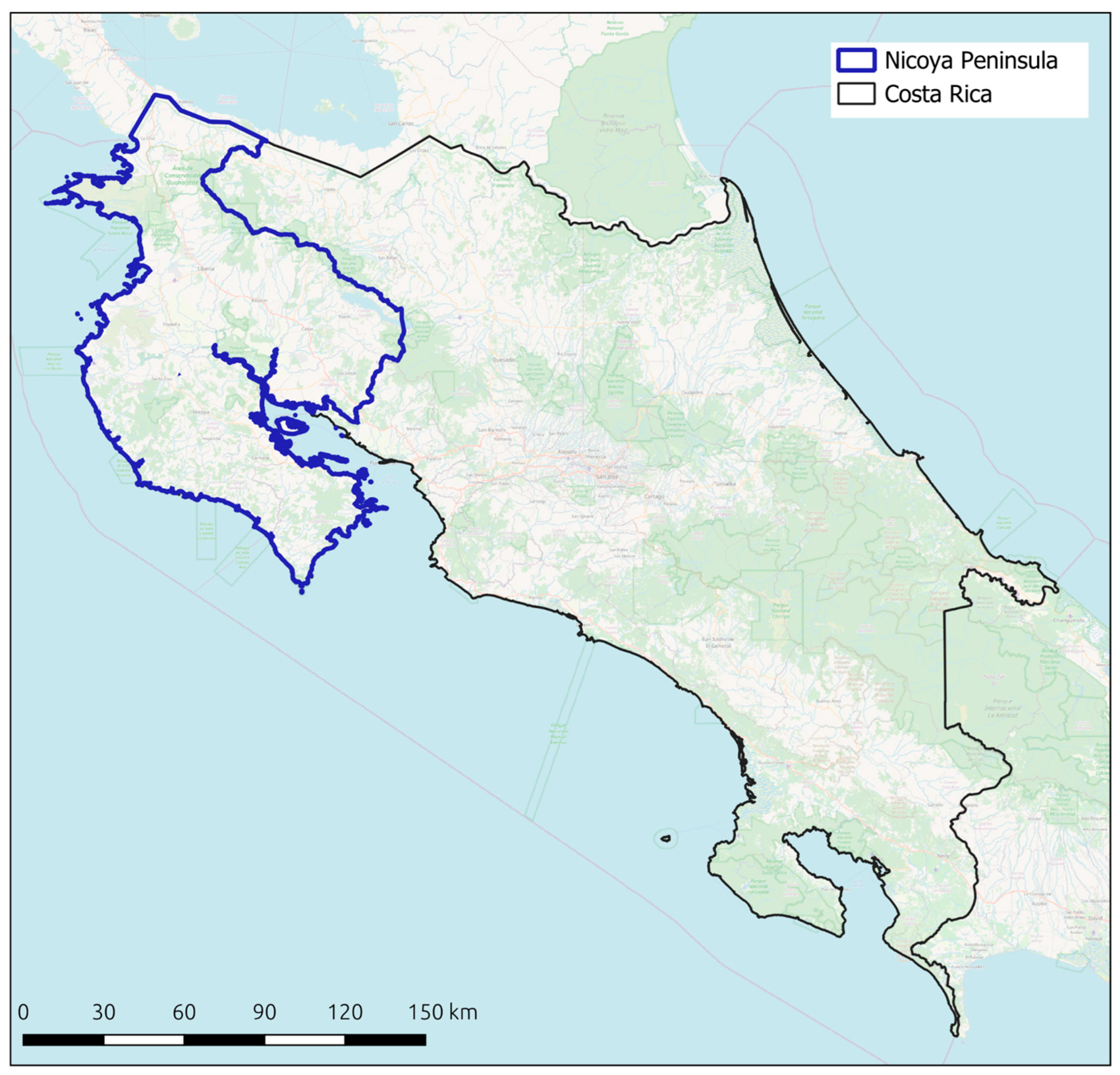
2.1. Costa Rica and the Nicoya Peninsula as a Case Study

Costa Rica (Figure 1) is home to ~5% of the world’s macroscopic species, with the greatest species density per 1000 km2 in the world [28]. As a relatively small country (surface area = 51,100 km2), its climate is influenced by both the Atlantic and the Pacific oceans. Its mean annual temperature varies from 27 °C on the north Pacific coast to 6 °C on the highest peak of the Cordillera. Total annual precipitation varies from 1300 mm to 7467 mm, and average monthly relative humidity varies between 65% and 90% [29]. Such orographic and climatic variation results in a tremendous diversity of ecosystems. The most recent classification suggests 14 major ecosystem types that range from the páramos (above the treeline), to seasonal tropical dry forests, evergreen tropical rainforests, mangroves, rivers and estuaries, bogs, marshes, and swamps [30]. The ecosystem diversity in the country, its high seasonality, and its data availability make it an excellent case study for evaluating how to improve EFT and EFD measurements for tropical areas.
To further compare EFT and EFD derivation at local vs. national extents, we conducted a regional analysis on the Nicoya Peninsula in the northwest of Costa Rica (Figure 1). We chose this region as it has the driest and most seasonally variable climate in the country [31], making it climatically distinct from the rest of the country—with potentially significant implications for the derivation for EFTs. The Nicoya Peninsula has a severe dry season from December to April with 0 mm of rain, and a short, mid-rainy-season drought in July and August. It also has two rainy seasons, with the most intense rains occurring in October and November [31]. Total annual precipitation varies from ~1500 mm to ~3000 mm over ~75 km, driving a shift from coastal wet forests to inland dry forests (Figure S1; [32]).
Climate projections suggest that the Nicoya Peninsula (Figure 1) may continue to grow more distinct in the future, with up to 25% declines in summer precipitation over the next century [33]. This region is also prone to floods and droughts, and a combination of deforestation, habitat conversion to agriculture, and climate drying are altering the biodiversity in the area, as well as the watershed dynamics [34,35]. As such, this area is a good test case for evaluating how well satellite imagery and remote sensing methods capture EFTs in highly seasonal and tropical environments, as well as in environments that are facing rapid environmental changes.

2.2. Satellite Data

Two satellite datasets were used in this study: MODIS (MOD13Q1 version 6) Enhanced Vegetation Index (EVI) and Landsat 7 EVI from 2001 to 2017. The MODIS EVI product offers 16-day composite images at a spatial resolution of 250 m. The Landsat EVI product offers an 8-day composite image at a spatial resolution of 30 m. These two datasets are available on the Google Earth Engine (GEE) platform [36]. EVI was chosen for this study, because it reduces sensitivity to soil and atmospheric effects and has been found to be less prone to saturation in temperate and tropical forests than other vegetation indices [37,38] and it is minimally sensitive to residual aerosol contamination from extensive fires in the Amazon and northern Asia [39]. This is particularly important in Costa Rica, because overall vegetation greenness is relatively high [40], which makes it more vulnerable to Normalized Difference Vegetation Index (NDVI) saturation, especially in the peak season. The period of 2001–2017 was chosen for several reasons: (1) Landsat-7 8-day EVI composites on GEE are only available until 2017; (2) MODIS 16-day EVI composites are only available from 2001; and (3) a 17-year period is adequate to represent long-term average vegetation productivity in the study area. Both time-series were homogenized to monthly time steps by using the monthly average for ease of comparison between them.

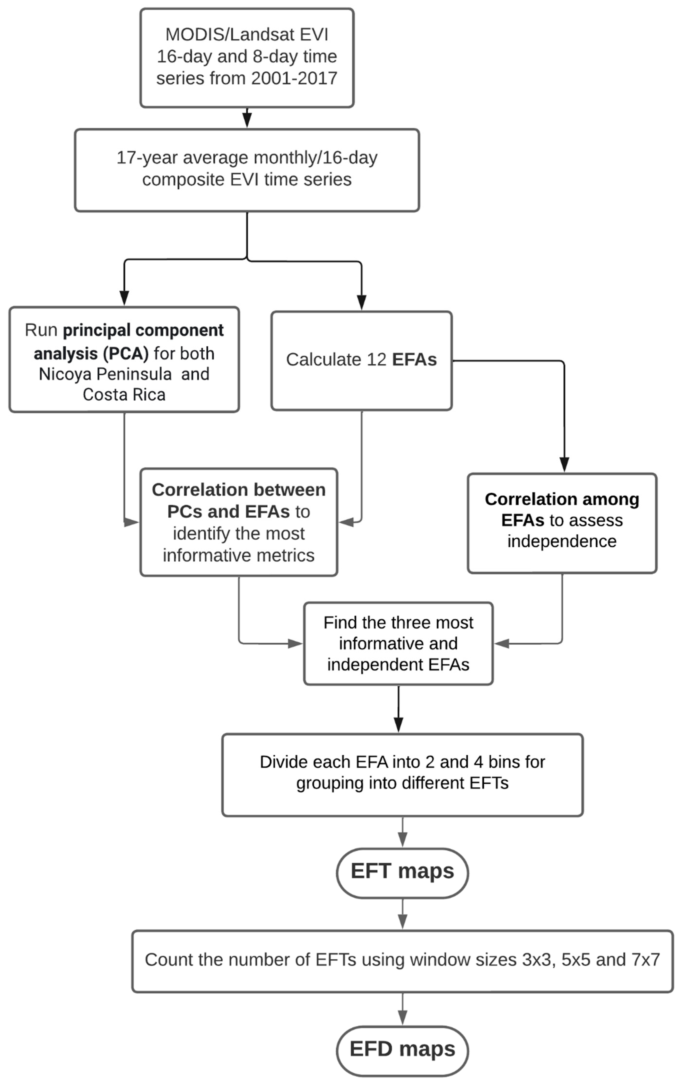
2.3. Obtaining Ecosystem Functional Types and Diversity

EFTs were derived based on the seasonal dynamics of carbon gains following Alcaraz-Segura et al. [7]. This approach includes five steps to derive EFTs (Figure 2): (1) principal components analysis, (2) calculating ecosystem functional attributes, (3) auto-correlation testing, (4) correlation between principal components and functional attributes to select the most predictive attributes, and (5) binning the functional attributes to develop an EFT classification. EFD Is then calculated using a moving window approach across the EFT map (see Cazorla et al. [4] for further details).
Several preprocessing steps were carried out prior to deriving EFTs. The 8-day Landsat EVI data were converted into 16-day composites to be consistent with MODIS. The monthly mean EVI was calculated for both MODIS and Landsat for each pixel over the 17-year period (2001–2017). Then, a principal component analysis (PCA) was run on the 17-year mean monthly EVI time series. The PCA allowed us to reduce the dimensionality of data, while retaining the important information from the original dataset. Eigenvalues were used to determine the explained variance for each PC. The eigenvectors were used to determine the relationships between PCs and monthly EVI values. In this study, the first three PCs were used, as combined they explained more than 99% percent of the variation in the dataset (Table S1).
Second, ecosystem functional attributes (EFAs) were calculated to determine the corresponding system features that could best be linked to the three most important PCs. The candidate EFAs include annual mean EVI, standard deviation (SD) of EVI, coefficient of variation (CV) of EVI, annual maximum EVI (Max), annual minimum EVI (Min), the dates at annual maximum and minimum EVI (DMax, DMin), and the dates of the start of growing season and end of growing season (SOS, EOS). The mean EVI, SD of EVI, and CV of EVI were derived from the 17-year average monthly EVI time series, and Max, Min, Dmax, Dmin, SOS, and EOS were derived from the 17-year average 16-day composite EVI time series for higher precision of these EFAs.
Third, auto-correlation testing among EFAs was applied to see how each EFA correlated with the others. This test helped us to avoid choosing very highly correlated EFAs to represent different PCs. There are two types of variables among the EFAs considered, linear variables, such as annual mean EVI and SD of EVI, and circular variables used to represent days of the year that repeat in an annual cycle, such as Dmax and Dmin. Therefore, three types of correlation coefficient statistical methods in this autocorrelation testing process were applied: (1) correlations between two linear variables, (2) correlations between a linear variable and a circular variable, and (3) correlations between two circular variables. These tests were performed using packages “Rfast” (https://cran.r-project.org/web/packages/Rfast/index.html, accessed on 15 May 2023) and “Hmisc” (https://cran.r-project.org/web/packages/Hmisc/index.html, accessed on 15 May 2023) in R. The circular EFAs were first converted into circular objects before calculating correlation coefficients.
Fourth, correlation coefficients between the first three PCs and all EFAs were calculated to determine which EFAs best represented the first three PCs. The most informative EFA for each PC was determined using the highest correlation coefficient. If the chosen EFA was highly correlated with an EFA in a previous step, the EFA with the second/third highest correlation coefficient was used. Finally, the three chosen EFAs were binned into categories to generate EFTs. In this study, the three chosen EFAs were EVI annual mean, EVI standard deviation (SD), and date of maximum EVI (DMax). Each EFA was split into both two bins and four bins to compare these classification approaches. Specifically, for the first and second EFA, which were annual mean EVI and SD of EVI, the middle quantiles were used to divide them into two bins (mean: denoted by 100 and 200; SD: denoted by 10, 20) and quartiles were used to divide them into four bins (mean: denoted by 100, 200, 300, 400; SD: denoted by 10, 20, 30, and 40). The third EFA, date of maximum EVI (DMax), was binned by examining the variable histograms and based on the authors’ (AE, JRS, KEL) field experience in the country. For two bins, the following breaks were used: bin 1 = DOY [day of year] 125–300, bin 2 = DOY 300–365 and 1–125. For four bins, we used: bin 1 = DOY 25–100, bin 2 = DOY 100–200, bin 3 = DOY 200–300, bin 4 = DOY 300–365 and 1–25. The three EFAs were grouped into eight different EFT classes denoted by 111, 112, 121, 122…222 when using two bins, and 64 classes denoted by 111, 112, 113, 114, 121, 122…444 when using four bins to represent the different EFTs. Both national EFTs and local EFTs were derived using the same three ecosystem functional attributes but with different breaks for the first two EFAs (annual mean EVI and SD of EVI). For nationally derived EFTs, the breaks were calculated using all pixels across Costa Rica, while for locally derived EFTs, the breaks were calculated using all pixels across the Nicoya Peninsula.
In total, four sets of EFTs were developed across Costa Rica (two sensors × two binning approaches), including MODIS-based and Landsat-based EFTs. The same four sets of EFTs (two sensors × two binning approaches) were also developed in the Nicoya Peninsula for assessing spatial extent impacts on identifying EFTs. Specifically, we repeated the principal component analysis, auto-correlation testing, and correlation coefficient estimates between PCs and EFAs within just the Nicoya Peninsula and found that the EFAs chosen for the Nicoya Peninsula were the same as those for the entire Costa Rica.
After deriving EFTs, Ecosystem Functional Diversity (EFD) was calculated by counting the number of EFTs within three moving window sizes, 3 × 3, 5 × 5, and 7 × 7 pixels, using the above eight sets of EFTs. The 30 m Landsat-derived EFD and 250 m MODIS-derived EFD were resampled into a 1 km resolution dataset to generate continuous values for EFD (rather than integers) when comparing across the different resolutions of data from the two sensors.

2.4. Comparison between MODIS-Based and Landsat-Based EFTs and EFDs in Costa Rica and EFTs and EFDs at National and Local Scales

To investigate the influences of sensors, classification approach (number of bins), window size, and spatial extent on the identification of EFTs and EFD, three types of comparisons were carried out. First, spatial maps of EFTs and EFD derived in different ways were visually compared. These comparisons included between MODIS and Landsat at the national scale of Costa Rica and within the Nicoya Peninsula, using the breaks derived either from the national or local binning. Second, pairwise scatter plots were generated to compare EFD values calculated using different sensors, numbers of bins, window size, and spatial extent. Third, the influence of spatial extent on the magnitude of EFD was investigated by comparing the distributions of values for nationally derived EFD with locally derived EFD for the Nicoya Peninsula. Specifically, a histogram was generated to show the number of pixels at different EFD levels at each spatial extent, and a Sankey diagram was created to show the correspondence between different levels of diversity for nationally derived and locally derived EFD.

3. Results

3.1. Ecosystem Functional Attributes (EFAs)

In this study, annual mean EVI, standard deviation (SD) of EVI, and DMax (date of maximum EVI) were found to be the three most important EFAs (Figures S2–S5). This is because the mean annual EVI has the highest correlation coefficient with the first principal component (PC) of the 17-year mean monthly EVI time series dataset. The SD of EVI and DMax have the highest correlation coefficient with the second and third PCs, respectively. In this study, the first three PCs were used, as combined they explained more than 99% of the variation in the dataset (Table S1).

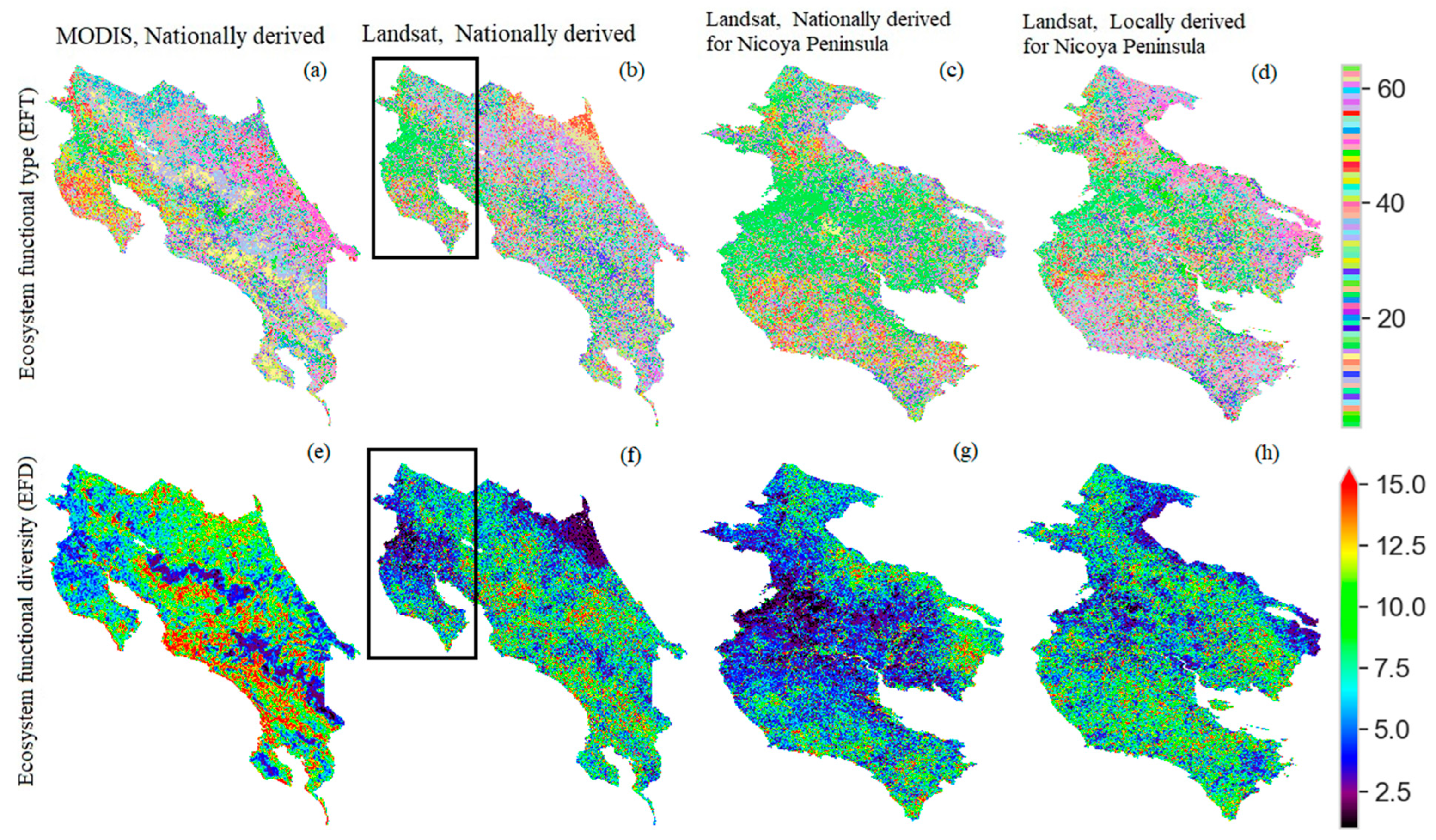
3.2. Ecosystem Functional Types (EFTs)

The sensor used to derive EFTs generated differences in the pattern of EFTs across Costa Rica (Figure 3a,b). The MODIS-derived EFTs map has dominant functional types shown in pink in Limón located in eastern Costa Rica while in the same province Landsat-derived EFT maps showed much more mixed types including in red, yellow, and pink. In the western portion of the country, particularly in Puntarenas, it also showed a very different EFTs pattern as MODIS-derived EFTs map showed the dominant types in yellow but Landsat-derived EFTs showed mixed types including in green, blue, and pink. In the center of the country, e.g., San José, the Landsat-derived EFT map has dominant types shown in blue that MODIS is missing. Overall, Landsat-derived EFTs showed greater granularity than those derived from MODIS.
The comparison of locally derived EFTs and nationally derived EFTs from the same sensor Landsat is presented in Figure 3c vs. Figure 3d to determine the effects of spatial extent on EFTs. Locally derived EFTs have a dominant functional type shown in bright green shared with the nationally derived EFTs in the same general area within the Nicoya Peninsula. EFTs derived at the local scale for the Nicoya Peninsula, however, show a wider range than those within the Nicoya Peninsula when derived at the national scale. Out of all 64 EFTs, only about 45 types derived at the national scale were present within the Nicoya Peninsula whereas all 64 EFTs are present when derived at the local scale. The dominant EFTs in pink are shown in the western and eastern border of the Nicoya Peninsula when derived at a local scale while this pattern was not found when derived at a national scale.

3.3. Ecosystem Functional Diversity (EFDs)

Despite the differences in EFTs, the national patterns of diversity (EFD) are fairly consistent between the two different sensors: highest diversity in the southwest (e.g., Puntarenas and San José), and lowest diversity in the Nicoya Peninsula (Figure 3e vs. Figure 3f). For MODIS, the values of EFD in the southwest of the country range from 12 to 15 but the values of EFD in the Nicoya Peninsula range from 3 to 7 (Figure 3e). Following a similar spatial pattern, the values of EFD derived from Landsat in the southwest of the country range from 7 to 12 while ranging from 1 to 5 in the Nicoya Peninsula (Figure 3f). Interestingly, in the middle of Costa Rica there are lower EFD values for MODIS (shown Figure 3e in blue) compared to Landsat (shown in Figure 3f in various colors). In addition, much lower EFDs values were found in the northeastern Limón from Landsat compared to those derived from MODIS (3 vs. 10). Noting that the area (and therefore potential heterogeneity) covered by a 7 × 7 MODIS window is larger than a 7 × 7 Landsat window, so MODIS is likely to capture greater functional diversity than Landsat. However, in the middle of Costa Rica there are lower EFD values for MODIS (shown Figure 3e in blue) compared to Landsat (shown in Figure 3f in various colors). This may be since these mountain areas were designated as protected areas, which allowed for continuous and homogeneous tree cover to remain at the 250 m scale.
The values of Landsat-based EFD in the Nicoya Peninsula are overall higher when derived at the local extent compared to the national extent (Figure 3g vs. Figure 3h). Specifically, the values of EFDs derived at a local extent range from 6 to 12 while these values at a national scale range from 3 to 6 in most of the Nicoya Peninsula. Along the eastern border of the Nicoya Peninsula (Figure 3h), there is a streak of low diversity (shown in blue) when derived locally that is absent from nationally derived EFD. In addition, the difference in diversity for the center compared to the tip of the Peninsula is greater for the national scale analysis compared to the local scale (Figure 3g vs. Figure 3h).

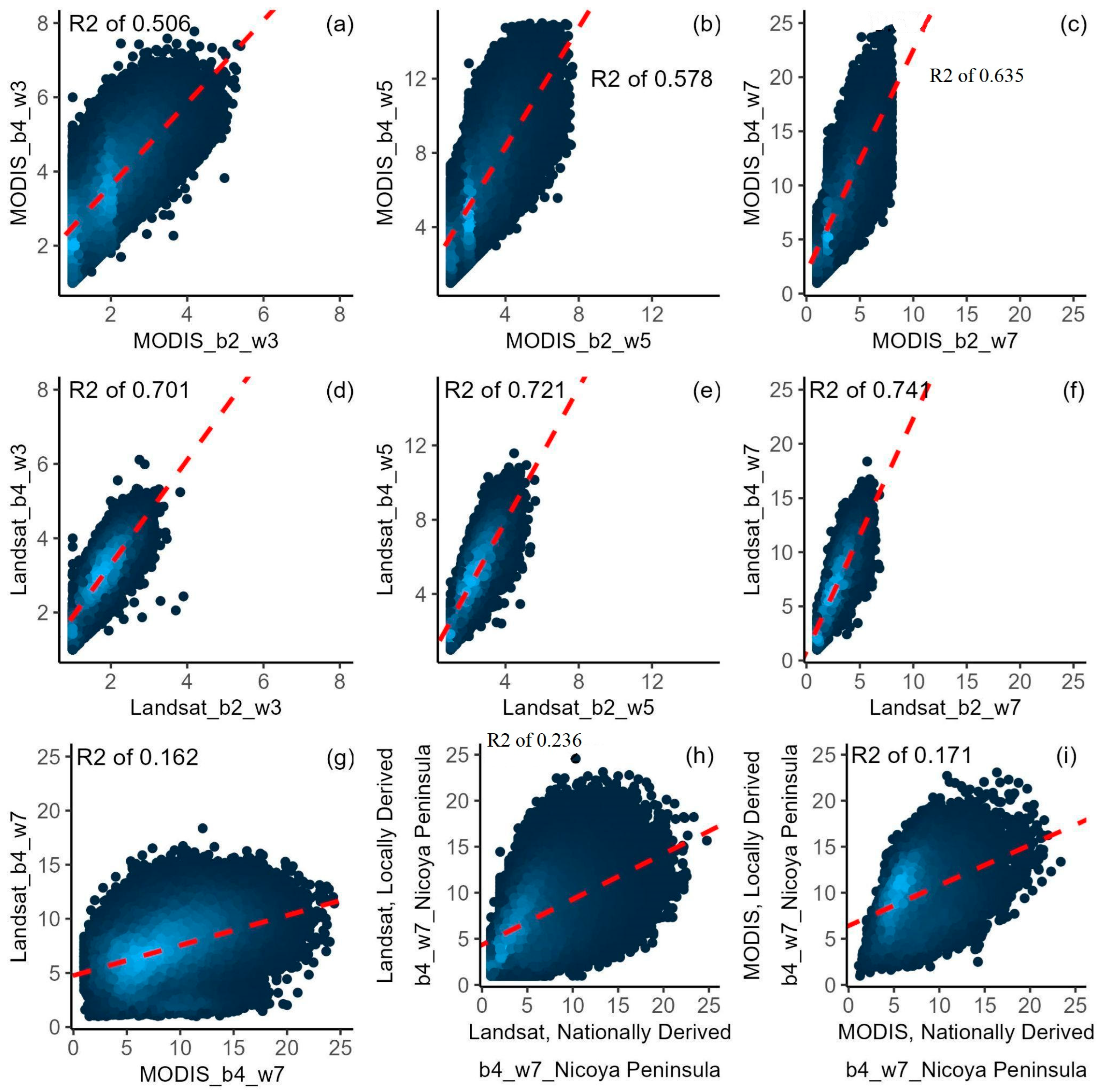
3.4. Comparison of EFDs Calculated Using Different Methods

The number of bins used (2 vs. 4) to categorize EFTs produces similar EFD for all tested window sizes (3, 5, and 7), with coefficients of determination (r2) for MODIS ranging from 0.51 to 0.64, increasing with window size (Figure 4a–c). Landsat data produce more consistent EFD values (r2 ranging from 0.70 to 0.74; Figure 4d–f), with the highest r2 values seen for the largest window size (Figure 4f). These results suggest that the number of bins used to classify EFTs had a limited influence on EFD, especially when using Landsat sensors.
A pixel-scale quantitative analysis showed that the Landsat-derived EFD was inconsistent with the MODIS-derived EFD (r2 = 0.16) (Figure 4g) when using the highest tested number of bins (4) and window size (7). In addition, national-scale-derived EFD in the Nicoya Peninsula does not correspond well with local-scale-derived EFD at a pixel scale. Specifically, the correlation coefficient (r2) is 0.24 (Figure 4h) for Landsat and 0.17 (Figure 4i) for MODIS, respectively.

3.5. Comparison of EFDs Calculated across Scales

Figure 5 shows that the values of EFD derived at the local scale are higher than when derived at the national scale. The number of pixels with higher diversity starting from a medium level at a local scale is higher than those extracted at a national scale (shown for Landsat-derived EFD; Figure 5a). The diversity levels derived at the smaller spatial extent appear to be nested within the diversity levels derived at a larger extent, with most pixels categorized as low diversity corresponding to low-medium or medium diversity pixels at a local scale, and many low-medium pixels nationally corresponding to medium and medium-high pixels locally (Figure 5b).

4. Discussion

The three key EFAs found in Costa Rica, annual mean EVI, standard deviation (SD) of EVI, and Dmax (date of maximum EVI), were consistent with several other recent case studies. For example, the same three EFAs (with a slight modification of seasonal coefficient of variation instead of standard deviation) were found to be the most informative in determining EFTs for the Baja California Peninsula, Mexico [4]. Another study from the Arctic tundra used two of the three same attributes (annual mean NDVI, date of maximum NDVI), along with date of maximum green-up as their EFAs [27]. Together, these studies suggest that the annual average greenness (annual mean EVI in this study) and date of peak greenness (Date of maximum EVI in this study) are general indicators of ecosystem functioning across very different biomes and should inform functional type mapping going forward.
Locally derived EFTs were found to have greater spatial heterogeneity. This is because there are more categories of locally classified EFAs than nationally classified EFAs (Figure S3d vs. Figure S3g; Figure S3e vs. Figure S3h). For example, for the first EFA (annual mean EVI) within the Nicoya Peninsula, most areas fell into the same bin in blue, at the national scale (Figure S3g), but were distributed across bins when EFTs were derived at the local scale (Figure S3d). The higher number of EFTs derived at a local scale would lead to higher values of EFD at most of the Nicoya Peninsula compared to nationally derived EFD.
However, there may be exceptions in a typical partial study area where one of the EFAs is much greater than it for the rest of the country. In this study, a streak of much lower diversity in the eastern border of the Nicoya Peninsula when derived locally was found compared to the nationally derived EFD. This is because the SD of EVI in the Nicoya Peninsula is much greater than in the rest of the country (Figure S2b). When the SD of EVI is broken down into four bins using breaks extracted from the Nicoya Peninsula, the SD values in the eastern border of the Nicoya Peninsula were all binned together (Figure S3e). However, when the SD of EVI is broken down into four bins using breaks from the entirety of Costa Rica, that particular area gets subsumed within a greater range of SD values (Figure S3h).
The selection of sensors for deriving EFTs and EFD is dependent on study area, data quality, and the application. For example, high spatial-resolution satellite data (such as 30 m Landsat) with good quality would be a good choice to detect EFTs and EFD; but in areas with limited good quality data (e.g., too many missing values due to cloud cover), MODIS (250 m) data may be a better choice due to its shorter revisiting time. However, Landsat has greater capacity to differentiate more EFTs than MODIS, particularly at the local scale (e.g., Nicoya Peninsula), due to its finer resolution (30 m).
Caution should be taken when choosing the spatial extent over which to derive these metrics. Our recommendation is to use extents that match the scale of the study question (i.e., derive EFD locally when the study area is small, like the Nicoya Peninsula, because it will better reflect the patterns unique to that area), and to consider carefully how to translate results between scales (e.g., when using regional or national EFT assessments on more local scales).
Using remote sensing to measure EFTs offers numerous advantages, but it is not without challenges. The main challenge is the categorical nature of the approach, which has been understood much better by testing the impact of two different bins, two sensor and spatial extents on deriving both EFTs and EFD in this study. However, these types of comparisons could be repeated with leaf area index (LAI), or fraction of photosynthetically active radiation (FPAR), or other measures of productivity, or other things that might respond to seasons, or that might respond functionally to their environment in different ways.
The lack of ground truth data for validating and refining the classifications can also be problematic. Our remotely sensed EFTs rely on spectral signatures and phenological patterns, which may not always align with ground-based observations, leading to potential inaccuracies in the results. These typically can be tested when vegetation indices are derived and published. More importantly for our purposes, validating the EFTs themselves present a challenge for validation because they are integrative and cannot be measured against a “truth”—the method is intended to delineate a pattern in functional behavior that is otherwise invisible. The best proof that the pattern is meaningful may come through management, if different functional types respond to different threats in different ways, or if greater EFD confers greater resilience to disturbance or change, or an overall increase in mean EVI under climate warming results in a reduction in functional diversity. These challenges underscore the importance of multi-scale, interdisciplinary approaches in ecosystem classification and monitoring.

5. Conclusions

Ecosystem functional types and ecosystem functional diversity have proven to be critical tools for helping to understand ecosystem-level biodiversity, but care should be taken in their application and interpretation. Our work adds to a growing body of literature in different biomes suggesting that EFAs could be promising for generating globally consistent EFT or EFD products, since three key EFAs (annual mean EVI, standard deviation of EVI, and date of annual maximum EVI) have now been found to be useful for several different study regions. However, researchers must consider the study area, data quality, and their application as a whole when choosing satellite sensors for deriving EFTs and EFD, as the spatial patterns of EFTs and EFD derived from different sensors can vary substantially. Moreover, researchers should choose spatial extents that match the scale of the study question (i.e., derive EFD locally when the study area is small), because it will better reflect the patterns unique to that region. Encouragingly, it appears that the derivation of EFTs is relatively robust regardless of the number of bins used to bin EFAs, as this process had a limited influence on EFD, especially when using Landsat sensors. These findings enable us to better understand these important methodological choices for deriving EFTs and EFD, how to use them more appropriately, and therefore help us improve systems for monitoring ecosystem functioning.
Moving forward, future research directions should focus on enhancing the effectiveness of remotely sensed EFT classifications by pairing this method with adaptive management, encompassing diverse ecosystem types, and testing the applicability of a broader range of sensors across varying scales. This approach will not only improve the accuracy of EFT mapping but also facilitate a more comprehensive understanding of ecosystem dynamics and their responses to environmental changes.

Supplementary Materials

The following supporting information can be downloaded at: https://www.mdpi.com/article/10.3390/rs15235593/s1.

Author Contributions

Conceptualization, L.L., J.R.S., A.H.A., D.A.-S., H.E.E. and R.C.-K.; Methodology, J.R.S., A.H.A., D.A.-S., H.E.E., A.E., K.E.L., R.J.P.S. and R.C.-K.; Formal analysis, J.R.S. and R.C.-K.; Data curation, L.L.; Writing—original draft, L.L. and R.C.-K.; Writing—review & editing, L.L., J.R.S., A.H.A., D.A.-S., H.E.E., A.E., K.E.L., R.J.P.S. and R.C.-K.; Visualization, J.R.S. and R.C.-K.; Funding acquisition, R.C.-K. All authors have read and agreed to the published version of the manuscript.

Funding

This work was funded by NASA (80NSSC18K0434, 80NSSC18K0446). Domingo Alcaraz Segura was supported by project PID2020-118041GB-I00 from the Spanish Research Projects Plan funded by MCIN/AEI/10.13039/501100011033/ and by FEDER funds “Una manera de hacer Europa”.

Data Availability Statement

The datasets were published https://zenodo.org/records/10235090.

Acknowledgments

We are indebted to our colleagues at the Natural Capital Project for their support. We thank Jim Zook and Pedro Juarez for valuable comments on the phenology and seasonality of Costa Rican landscapes.

Conflicts of Interest

The authors declare no conflict of interest.

References

  1. Mucina, L. Biome: Evolution of a Crucial Ecological and Biogeographical Concept. New Phytol. 2019, 222, 97–114. [Google Scholar] [CrossRef] [PubMed]
  2. Alcaraz, D.; Paruelo, J.; Cabello, J. Identification of Current Ecosystem Functional Types in the Iberian Peninsula. Glob. Ecol. Biogeogr. 2006, 15, 200–212. [Google Scholar] [CrossRef]
  3. Paruelo, J.M.; Jobbágy, E.G.; Sala, O.E. Current Distribution of Ecosystem Functional Types in Temperate South America. Ecosystems 2001, 4, 683–698. [Google Scholar] [CrossRef]
  4. Cazorla, B.P.; Cabello, J.; Peñas, J.; Garcillán, P.P.; Reyes, A.; Alcaraz-Segura, D. Incorporating Ecosystem Functional Diversity into Geographic Conservation Priorities Using Remotely Sensed Ecosystem Functional Types. Ecosystems 2021, 24, 548–564. [Google Scholar] [CrossRef]
  5. Fernández, N.; Paruelo, J.M.; Delibes, M. Ecosystem Functioning of Protected and Altered Mediterranean Environments: A Remote Sensing Classification in Doñana, Spain. Remote Sens. Environ. 2010, 114, 211–220. [Google Scholar] [CrossRef]
  6. Ivits, E.; Cherlet, M.; Mehl, W.; Sommer, S. Ecosystem Functional Units Characterized by Satellite Observed Phenology and Productivity Gradients: A Case Study for Europe. Ecol. Indic. 2013, 27, 17–28. [Google Scholar] [CrossRef]
  7. Alcaraz-Segura, D.; Paruelo, J.M.; Epstein, H.E.; Cabello, J. Environmental and Human Controls of Ecosystem Functional Diversity in Temperate South America. Remote Sens. 2013, 5, 127–154. [Google Scholar] [CrossRef]
  8. Cabello, J.; Alcaraz-Segura, D.; Altesor, A.; Delibes, M.; Baeza, S.; Liras, E. Funcionamiento Ecosistémico y Evaluación de Prioridades Geográficas En Conservación. Ecosistemas 2008, 17, 53–63. [Google Scholar]
  9. Cabello, J.; Lourenço, P.; Reyes, A.; Alcaraz-Segura, D. Ecosystem Services Assessment of National Parks Networks for Functional Diversity and Carbon Conservation Strategies Using Remote Sensing. Earth Obs. Ecosyst. Serv. 2013, 179, 430. [Google Scholar]
  10. Paruelo, J.; Alcaraz-Segura, D.; Volante, J.N. El seguimiento del nivel de provisión de los servicios ecosistémicos. Expans. E Intensificación Agríc. En Argent. Valorac. Bienes Serv. Ecosistémicos Para El Ordenamiento Territ. Ed INTA B. Aires. 2011. Available online: https://www.researchgate.net/profile/Esteban-Jobbagy/publication/249643891_Valoracion_de_Servicios_Ecosistemicos_Conceptos_herramientas_y_aplicaciones_para_el_ordenamiento_territorial/links/0deec51e963480928c000000/Valoracion-de-Servicios-Ecosistemicos-Conceptos-herramientas-y-aplicaciones-para-el-ordenamiento-territorial.pdf#page=147 (accessed on 25 September 2023).
  11. Volante, J.N.; Alcaraz-Segura, D.; Mosciaro, M.J.; Viglizzo, E.F.; Paruelo, J.M. Ecosystem Functional Changes Associated with Land Clearing in NW Argentina. Agric. Ecosyst. Environ. 2012, 154, 12–22. [Google Scholar] [CrossRef]
  12. Oki, T.; Blyth, E.M.; Berbery, E.H.; Alcaraz-Segura, D. Land Use and Land Cover Changes and Their Impacts on Hydroclimate, Ecosystems and Society. In Climate Science for Serving Society; Springer: Berlin/Heidelberg, Germany, 2013; pp. 185–203. [Google Scholar]
  13. Müller, O.V.; Berbery, E.H.; Alcaraz-Segura, D.; Ek, M.B. Regional Model Simulations of the 2008 Drought in Southern South America Using a Consistent Set of Land Surface Properties. J. Clim. 2014, 27, 6754–6778. [Google Scholar] [CrossRef]
  14. Potter, C.S.; Brooks, V. Global Analysis of Empirical Relations between Annual Climate and Seasonality of NDVI. Int. J. Remote Sens. 1998, 19, 2921–2948. [Google Scholar] [CrossRef]
  15. Zhang, X.; Friedl, M.A.; Schaaf, C.B.; Strahler, A.H.; Hodges, J.C.F.; Gao, F.; Reed, B.C.; Huete, A. Monitoring Vegetation Phenology Using MODIS. Remote Sens. Environ. 2003, 84, 471–475. [Google Scholar] [CrossRef]
  16. Pérez-Hoyos, A.; Martínez, B.; García-Haro, F.J.; Moreno, Á.; Gilabert, M.A. Identification of Ecosystem Functional Types from Coarse Resolution Imagery Using a Self-Organizing Map Approach: A Case Study for Spain. Remote Sens. 2014, 6, 11391–11419. [Google Scholar] [CrossRef]
  17. Wang, Y.; Huang, F. Identification and Analysis of Ecosystem Functional Types in the West of Songnen Plain, China, Based on Moderate Resolution Imaging Spectroradiometer Data. J. Appl. Remote Sens. 2015, 9, 096096. [Google Scholar] [CrossRef]
  18. Cadotte, M.W.; Carscadden, K.; Mirotchnick, N. Beyond Species: Functional Diversity and the Maintenance of Ecological Processes and Services. J. Appl. Ecol. 2011, 48, 1079–1087. [Google Scholar] [CrossRef]
  19. Díaz, S.; Lavorel, S.; Chapin, F.S.; Tecco, P.A.; Gurvich, D.E.; Grigulis, K. Functional Diversity—At the Crossroads between Ecosystem Functioning and Environmental Filters. In Terrestrial Ecosystems in a Changing World; Springer: Berlin/Heidelberg, Germany, 2007; pp. 81–91. [Google Scholar]
  20. Balvanera, P.; Pfisterer, A.B.; Buchmann, N.; He, J.-S.; Nakashizuka, T.; Raffaelli, D.; Schmid, B. Quantifying the Evidence for Biodiversity Effects on Ecosystem Functioning and Services. Ecol. Lett. 2006, 9, 1146–1156. [Google Scholar] [CrossRef] [PubMed]
  21. Díaz, S.; Fargione, J.; Chapin III, F.S.; Tilman, D. Biodiversity Loss Threatens Human Well-Being. PLoS Biol. 2006, 4, e277. [Google Scholar] [CrossRef]
  22. Duncan, C.; Thompson, J.R.; Pettorelli, N. The Quest for a Mechanistic Understanding of Biodiversity–Ecosystem Services Relationships. Proc. R. Soc. B Biol. Sci. 2015, 282, 20151348. [Google Scholar] [CrossRef]
  23. Mouchet, M.A.; Villéger, S.; Mason, N.W.H.; Mouillot, D. Functional Diversity Measures: An Overview of Their Redundancy and Their Ability to Discriminate Community Assembly Rules. Funct. Ecol. 2010, 24, 867–876. [Google Scholar] [CrossRef]
  24. Proença, V.; Martin, L.J.; Pereira, H.M.; Fernandez, M.; McRae, L.; Belnap, J.; Böhm, M.; Brummitt, N.; García-Moreno, J.; Gregory, R.D. Global Biodiversity Monitoring: From Data Sources to Essential Biodiversity Variables. Biol. Conserv. 2017, 213, 256–263. [Google Scholar] [CrossRef]
  25. Skidmore, A.K.; Coops, N.C.; Neinavaz, E.; Ali, A.; Schaepman, M.E.; Paganini, M.; Kissling, W.D.; Vihervaara, P.; Darvishzadeh, R.; Feilhauer, H. Priority List of Biodiversity Metrics to Observe from Space. Nat. Ecol. Evol. 2021, 5, 896–906. [Google Scholar] [CrossRef] [PubMed]
  26. Pereira, H.M.; Ferrier, S.; Walters, M.; Geller, G.N.; Jongman, R.H.G.; Scholes, R.J.; Bruford, M.W.; Brummitt, N.; Butchart, S.H.M.; Cardoso, A.C. Essential Biodiversity Variables. Science 2013, 339, 277–278. [Google Scholar] [CrossRef] [PubMed]
  27. Epstein, H.; Armstrong, A.; Alcaraz-Segura, D.; Tassone, M.; Raynolds, M. Assessing the Controls on Ecosystem Functional Diversity in the Arctic Tundra at Circumpolar and Regional Scales. In Proceedings of the AGU Fall Meeting Abstracts, New Orleans, LA, USA, 13–17 December 2021; Volume 2021, p. B13A-01. [Google Scholar]
  28. Obando, V. Biodiversidad En Costa Rica: Estado Del Conocimiento y Gestión; INBio: Heredia, CR, USA, 2002. [Google Scholar]
  29. Herrera, W. Climate of Costa Rica. In Costa Rican Ecosystems; The University of Chicago Press: Chicago, IL, USA, 2016; pp. 19–29. [Google Scholar]
  30. Kappelle, M. Costa Rica’s Ecosystems: Setting the Stage. In Costa Rican Ecosystems; The University of Chicago Press: Chicago, IL, USA, 2016; p. 3. [Google Scholar]
  31. Steyn, D.G.; Moisseeva, N.; Harari, O.; Welch, W.J. Temporal and Spatial Variability of Annual Rainfall Patterns in Guanacaste, Costa Rica. Available online: https://open.library.ubc.ca/collections/52383/items/1.0340318 (accessed on 25 September 2023).
  32. Fick, S.E.; Hijmans, R.J. WorldClim 2: New 1-km Spatial Resolution Climate Surfaces for Global Land Areas. Int. J. Climatol. 2017, 37, 4302–4315. [Google Scholar] [CrossRef]
  33. Rauscher, S.A.; Giorgi, F.; Diffenbaugh, N.S.; Seth, A. Extension and Intensification of the Meso-American Mid-Summer Drought in the Twenty-First Century. Clim. Dyn. 2008, 31, 551–571. [Google Scholar] [CrossRef]
  34. Hund, S.V.; Grossmann, I.; Steyn, D.G.; Allen, D.M.; Johnson, M.S. Changing Water Resources under El Niño, Climate Change, and Growing Water Demands in Seasonally Dry Tropical Watersheds. Water Resour. Res. 2021, 57, e2020WR028535. [Google Scholar] [CrossRef]
  35. Karp, D.S.; Frishkoff, L.O.; Echeverri, A.; Zook, J.; Juárez, P.; Chan, K.M. Agriculture Erases Climate-driven Β-diversity in Neotropical Bird Communities. Glob. Chang. Biol. 2018, 24, 338–349. [Google Scholar] [CrossRef]
  36. Amani, M.; Ghorbanian, A.; Ahmadi, S.A.; Kakooei, M.; Moghimi, A.; Mirmazloumi, S.M.; Moghaddam, S.H.A.; Mahdavi, S.; Ghahremanloo, M.; Parsian, S.; et al. Google Earth Engine Cloud Computing Platform for Remote Sensing Big Data Applications: A Comprehensive Review. IEEE J. Sel. Top. Appl. Earth Obs. Remote Sens. 2020, 13, 5326–5350. [Google Scholar] [CrossRef]
  37. Huete, A.R.; Didan, K.; Shimabukuro, Y.E.; Ratana, P.; Saleska, S.R.; Hutyra, L.R.; Yang, W.; Nemani, R.R.; Myneni, R. Amazon Rainforests Green-up with Sunlight in Dry Season. Geophys. Res. Lett. 2006, 33. [Google Scholar] [CrossRef]
  38. Xiao, X.; Hollinger, D.; Aber, J.; Goltz, M.; Davidson, E.A.; Zhang, Q.; Moore, B. Satellite-Based Modeling of Gross Primary Production in an Evergreen Needleleaf Forest. Remote Sens. Environ. 2004, 89, 519–534. [Google Scholar] [CrossRef]
  39. Xiao, X.; Braswell, B.; Zhang, Q.; Boles, S.; Frolking, S.; Moore, B. Sensitivity of Vegetation Indices to Atmospheric Aerosols: Continental-Scale Observations in Northern Asia. Remote Sens. Environ. 2003, 84, 385–392. [Google Scholar] [CrossRef]
  40. Kappelle, M. Costa Rican Ecosystems; University of Chicago Press: Chicago, IL, USA, 2016. [Google Scholar]
Figure 1. Map of study area. The black line is the Costa Rica boundary and the blue line is the Nicoya Peninsula boundary.
Remotesensing 15 05593 g001
Figure 2. Workflow for generating Ecosystem Functional Types (EFTs) and Ecosystem Functional Diversity (EFD) from satellite time series of the Enhanced Vegetation Index (EVI), involving relating the principal components (PCs) from a principal components analysis to key Ecosystem Functional Attributes (EFA).
Remotesensing 15 05593 g002
Figure 3. Spatial patterns of Ecosystem Functional Types (EFT) and Ecosystem Functional Diversity (EFD), derived with different sensors and methods. EFT maps were derived at the national scale for Costa Rica, using MODIS (a) and Landsat (b). Box inset in (b) represents the Nicoya Peninsula and is shown as a close-up in (c) and using Landsat at the local scale (d). Maps of EFD correspond to the EFT maps in the row above, for MODIS (e) and Landsat (f,g) at the national scale and for Landsat at the local scale (h) in the Nicoya Peninsula. All EFTs shown here were derived using four bins to divide functional variables (annual mean EVI, standard deviation of EVI, and date of annual maximum EVI); all EFDs were derived using a window size of 7 × 7 pixels (described in Figure 1). The number on the EFT legend (EFT row) represents different EFTs, with higher numbers corresponding to EFTs with higher mean EVI; the number on the EFD legends (EFD row) represents the number of EFTs in the window size of 7 × 7 pixels.
Remotesensing 15 05593 g003
Figure 4. Comparison of Ecosystem Functional Diversity (EFD) calculated using different methods to derive Ecosystem Functional Type (EFT). Methods to derive EFT were based on dividing the functional variables into 2 (b2) vs. 4 (b4) bins, using different window sizes to count the number of functional types, either 3 × 3 (w3), 5 × 5 (w5), or 7 × 7 (w7) pixels. The top two rows show comparisons of EFD using EFTs derived from MODIS (ac), and Landsat (df) at national scales. Comparison between MODIS and Landsat-based EFD (g) at the national scale are shown for the method of 4 bins and a window size of 7, as this had the highest coefficient of determination (R2); all other MODIS vs. Landsat comparisons can be found in the Supplemental Materials in Figure S6. Comparison of EFD for EFTs derived at the local (Nicoya Peninsula) scale vs. the national (Costa Rica) scale ((h) based on Landsat and (i) based on MODIS) is likewise only shown for 4 bins, with a window size of 7; all other comparisons can be found in Supplemental Figure S8. Red dashed line represents a linear trend.
Remotesensing 15 05593 g004
Figure 5. Comparison of Ecosystem Functional Diversity (EFD) derived at national and local scales. The histogram shows the frequency (number of pixels) of different levels of diversity for EFDs derived at the national scale and local scale in the Nicoya Peninsula (a). The Sankey diagram (b) is constructed from the same dataset as (a) and shows how locally derived EFD (on the right) is nested within nationally derived EFD (on the left). The EFD shown here was derived from 30 m Landsat using 4 bins to classify EFT and a window size of 7 (see Figure 2 for full description of method).
Remotesensing 15 05593 g005
Disclaimer/Publisher’s Note: The statements, opinions and data contained in all publications are solely those of the individual author(s) and contributor(s) and not of MDPI and/or the editor(s). MDPI and/or the editor(s) disclaim responsibility for any injury to people or property resulting from any ideas, methods, instructions or products referred to in the content.

