Technical Note

A New Approach to the Ionosphere at Middle and Low Latitudes under the Geomagnetic Quiet Time of December 2019 by ICON and GOLD Observations

1
College of Astronautics, Nanjing University of Aeronautics and Astronautics, Nanjing 211106, China
2
Planetary Environmental and Astrobiological Research Laboratory (PEARL), School of Atmospheric Sciences, Sun Yat-sen University, Zhuhai 519082, China
3
Key Laboratory of Earth and Planetary Physics, Institute of Geology and Geophysics, Chinese Academy of Sciences, Beijing 100029, China
4
College of Earth and Planetary Sciences, University of the Chinese Academy of Sciences, Beijing 100049, China
5
Heilongjiang Mohe National Observatory of Geophysics, Institute of Geology and Geophysics, Chinese Academy of Sciences, Beijing 100029, China
6
Beijing National Observatory of Space Environment, Institute of Geology and Geophysics, Chinese Academy of Sciences, Beijing 100029, China
7
Shandong Key Laboratory of Optical Astronomy and Solar-Terrestrial Environment, School of Space Science and Physics, Institute of Space Sciences, Shandong University, Weihai 264209, China
*
Author to whom correspondence should be addressed.
Remote Sens. 2023, 15(23), 5591; https://doi.org/10.3390/rs15235591
Submission received: 4 November 2023 / Revised: 27 November 2023 / Accepted: 29 November 2023 / Published: 1 December 2023

Abstract

:
It has been found that the total electron content (TEC) and the ionospheric electric fields indicated by the geomagnetic data showed inconsistent changes with each other at the mid- and low latitudes in both the American and the Asian–Australian sectors during geomagnetic quiet time (GQT) from 30 November to 8 December 2019 (Kpmax = 1.7). Meanwhile, the effects of thermospheric compositions are still indistinct. In this work, we analyze the mid/low-latitude ionospheric variations during this period, utilizing multi-instrument observations. The vertical drift velocities from the Ionospheric Connection Explorer (ICON) show significant variations and are in line with the changes in TEC at low latitudes in both of the two sectors. The zonal electric fields are supposed to play the main role in the TEC changes. This is also confirmed by the ionospheric F2 layer parameters data from the ionosonde stations at Sanya in the Asian–Australian sectors. The correlation between the variations in the geomagnetic H component (ΔH) and ionospheric F-layer electric fields can be affected by solar activity levels. The geomagnetic data ΔH sometimes may not indicate the magnitude of the electric fields in the F-region ionosphere under geomagnetic quiet conditions. The column density ratio of atomic oxygen (O) to molecular nitrogen (N2) (∑O/N2) from the Global Scale Observations of the Limb and Disk (GOLD) showed a strong enhancement at mid-latitudes in the American sector on 30 November. It is speculated that the neutral compositions should make a minor contribution to the changes in TEC during this event, compared with the electric fields.

Graphical Abstract

1. Introduction

The ionosphere is an important region of the solar-terrestrial space, accompanied by complex temporal and spatial changes. The variations in ionospheric parameters are closely related to solar activity, geomagnetic disturbances, lower atmospheric forcing, and so on [1,2,3,4,5,6,7]. The characterizations of ionospheric disturbances have been an important subject of ionospheric physics and a major challenge for space weather prediction in past decades [8,9,10].
During the periods generally considered to be geomagnetic quiet time (GQT), the ionosphere has also shown large daily variations [11,12,13,14,15,16,17,18,19,20,21,22]. In studies from recent years, ionospheric disturbances may be associated with variations in the electric field or thermosphere composition during the GQT. Xiong et al. [23] investigated an anomalous ionospheric disturbance in Eastern Asian during the geomagnetic quiet day in November 2016. They noted that the enhancement of the equatorial electric field led to the decline in total electron content (TEC) at low latitudes and the enhancement at middle latitudes. The case of the ionospheric electron density enhancement was studied by Liu et al. [24] and they found that the equatorial zonal electric fields played an important role at low latitudes. Cai et al. [25] reported changes in thermospheric composition and ionospheric TEC during the magnetically quiet period (maximum Kp = 1.7) in the mid-latitudes. They found that the column density ratio of atomic oxygen (O) to molecular nitrogen (N2) (∑O/N2) and TEC showed similar changes. Cai et al. [26] studied the influences of the interplanetary magnetic field (IMF) on the middle thermospheric composition during the GQT using the National Center for Atmospheric Research (NCAR) thermosphere–ionosphere–electrodynamics general circulation model (TIE-GCM) and ∑O/N2 data from Global Scale Observations of the Limb and Disk (GOLD). They found that the dominant By could lead to strong disturbances in the thermospheric compositions and propagate into mid-latitudes during these times. Nevertheless, more studies about the relevant mechanisms, energy sources, and the complete processes of related effects are still needed using observations and simulations.
Kuai et al. [1] investigated ionospheric disturbances at mid/low latitudes during a geomagnetic quiet period from 30 November to 8 December 2019 (Kpmax = 1.7). They found that the TEC had complex changes in the mid/low latitudes in both the American and the Asian–Australian sectors. They also observed low-latitude electric field variations using the geomagnetic data. A significant daily variability in the tidal winds is thought to drive the changes in the Ionospheric F-region electric fields during the quiescent period. However, it is worth noting that the TEC and the deviations (ΔH) in the geomagnetic horizontal (H) component were inconsistent in both sectors, especially from December 4 to 6. The findings of Kuai et al. [1] raised an interesting question: does the inconsistency of the change in TEC with ΔH imply that the effects of the F-region electric field variation on ionospheric TEC deviate from the prevailing perception, or that there are unclarified mechanistic processes?
In addition, the ∑O/N2 observed by TIMED/GUVI were seriously incomplete during this case. They suggested that there was little change in the thermospheric compositions at mid/low latitudes during the period according to partial available data. What are the more accurate features of changes in the mid/low-latitude thermosphere components during this period? What are the effects of changes in thermosphere composition on TEC variations in this event? In summary, the effects of the ionospheric F-region electric fields and thermospheric compositions for this event are still unclear and require further research.
In recent years, continuously updated detection methods such as satellites have provided more observations on the ionosphere, and the above event can also be further explored. In order to better understand the effects of the changes in the F-region ionospheric electric field on the TEC variations, we used the vertical plasma drift from the Ionospheric Connection Explorer (ICON) to reflect the electric field changes during the GQT from 30 November to 8 December 2019 in this study. The ∑O/N2 data from GOLD were used to observe and further analyze the changes in the thermospheric composition in the American sector during this event.

2. Dataset

Solar wind data are supplied by the Advanced Composition Explorer (ACE) satellite, which was launched by the United States in August 1997 and can give real-time solar wind parameters [27]. The Kp index is used to represent the geomagnetic conditions. The symmetric component of the ring current index (SYM-H) can be considered as a version with a 1 min time resolution of the Dst index [28].
The E×B drift in the F region of the equatorial ionosphere can characterize the zonal electric field and is positively correlated with the equatorial electrojet (EEJ) strength during the daytime. The EEJ can be estimated using the deviations (ΔH) of the geomagnetic horizontal (H) component between magnetometers at equatorial and off-equatorial stations [29], and thus characterize the dayside zonal electric field.
The Global Navigation Satellite Systems (GNSS) TEC data can be obtained from the Massachusetts Institute of Technology (MIT) Haystack Observatory Madrigal database (http://www.openmadrigal.org, accessed on 18 November 2023.) [30]. The MIT TEC has a resolution of 1° × 1° and a time resolution of 5 min. TEC are the integrals of the ionospheric electron density in the height direction, and can be used to represent the variations in the ionospheric electron density.
The vertical plasma drift data are given by ICON spacecraft. The spacecraft operated in a low-inclination (~27°) circular orbit at ~575 km altitude. The ICON uses an ion velocity meter (IVM) to measure the ion drift motion at the satellite altitude with an accuracy of 7.5 m/s [31,32,33]. The vertical plasma drift data within 15° of the magnetic equator during the daytime is very accurate. In this work, we use plasma drift data from IVM Level 2 version 6. We chose the data based on the flags (ICON_L27_RPA_Flag and ICON_L27_DM_Flag) equal to 0 to ensure data quality [34]. The vertical plasma drift data from ICON used in this work were measured in the altitude range of ~579–604 km. Positive values for the vertical drift indicate upward movement. Eastward electric fields can cause upward vertical plasma drift.
The ∑O/N2 data are offered by GOLD. The GOLD carries the SES-14 communication satellite in a geostationary orbit. The GOLD imaging spectrograph can measure the Earth’s emissions in the range of 132 to 162 nm. The mission repeatedly observed the same hemisphere, allowing a clear distinction between spatial and temporal variations in the Americas [35]. GOLD can scan the full disk with a 0.5 h resolution in the geographic range of ~±70° in latitude and longitude relative to the spacecraft nadir, covering areas from about 120°W to 20°E and 70°S to 70°N [20]. The ∑O/N2 data are sourced from the OI 135.6 nm and the N2 LBH brightness during the daytime. Disk images of ∑O/N2 have a 250 km × 250 km spatial resolution (at nadir) and a precision of 10% [36,37].
We also use foF2 and hmF2 data at Sanya (109.6°E, 18.3°N), recorded with a Lowell DPS-4D ionosonde. The foF2 is the F2-layer critical frequency and the hmF2 is the height of the F2-layer maximum electron density. The foF2 and hmF2 can be obtained by using the true height inversion algorithm constructed in the SAO-Explorer software 3.6 [38].
Compared to Kuai et al. [1], the vertical plasma drift data from ICON, ∑O/N2 data from GOLD, and foF2 and hmF2 data at Sanya (109.6°E, 18.3°N) are newly added in this work. Other data are processed in agreement with Kuai et al. [1].

3. Results and Discussion

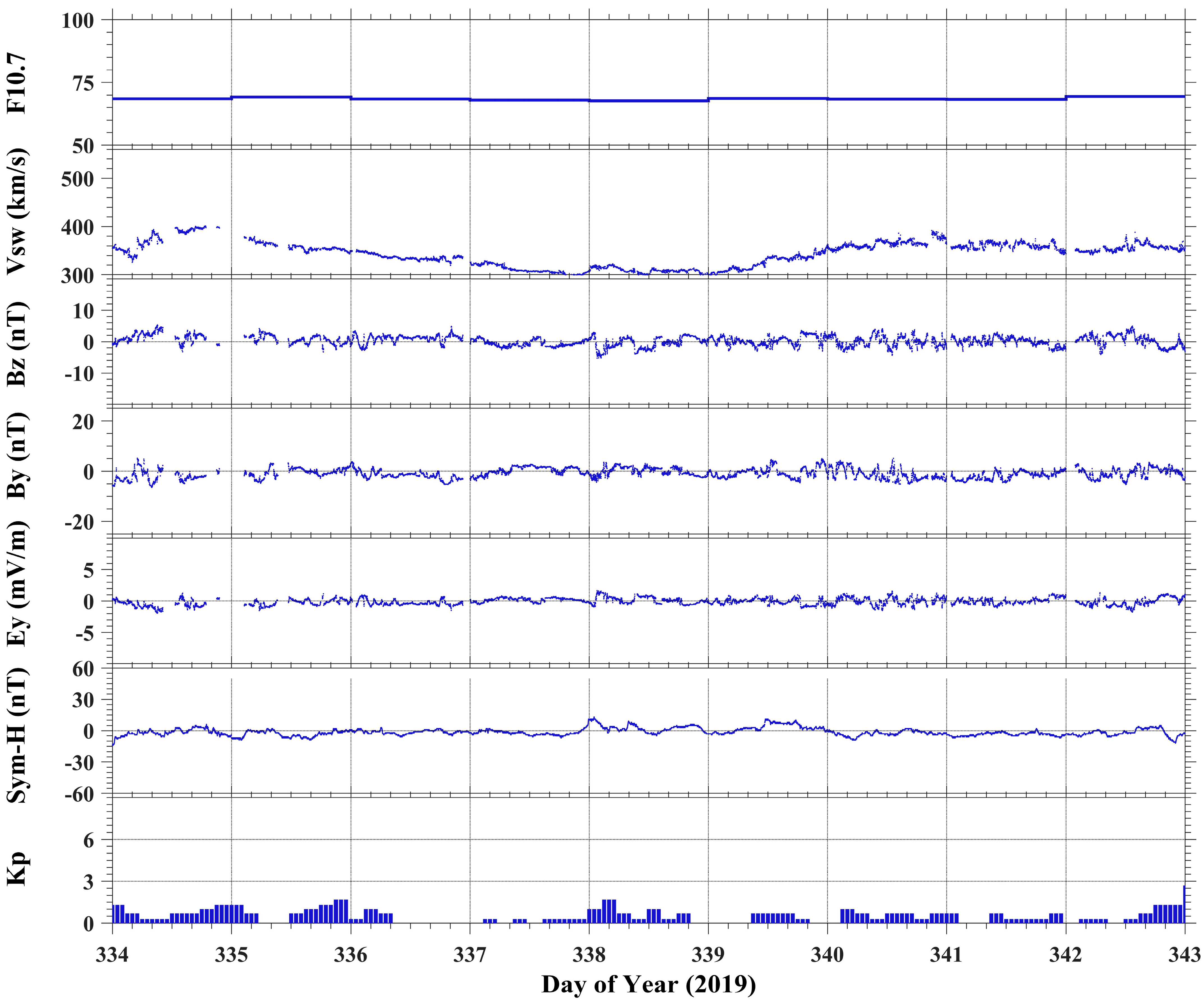
3.1. Geomagnetic Conditions during this Period

Figure 1 shows the variations in geomagnetic condition parameters from 30 November to 8 December 2019, including the F10.7 index, the solar wind speed velocity (VSW), the interplanetary magnetic field (IMF) Bz and By components, Ey, SYM-H index, and Kp index. During the GQT, the values of the F10.7 index were ~68 units. The values of the AE index were essentially below 200 nT and the values of IMF (By and Bz) were ~0 nT. It is worth noting that |By| > |Bz| during ~0000–0450 UT, 0700–0838 UT, 1320–1830 UT on November 30, ~0400–0700 UT, 0800–0900 UT, 1000–1420 UT, 2000–2400 UT on 1 December, and ~0300–0350 UT, 0750–0940 UT, 1200–2230 UT on 2 December. By was the dominant component of IMF when |By| > |Bz|. Furthermore, the values of the Kp index were mostly <1 (Kpmax = 1.7) and the minimum value of the SYM-H index was still greater than −10. In other words, all the solar activity, the auroral energy input, and the geomagnetic activity were at very low levels in this case.

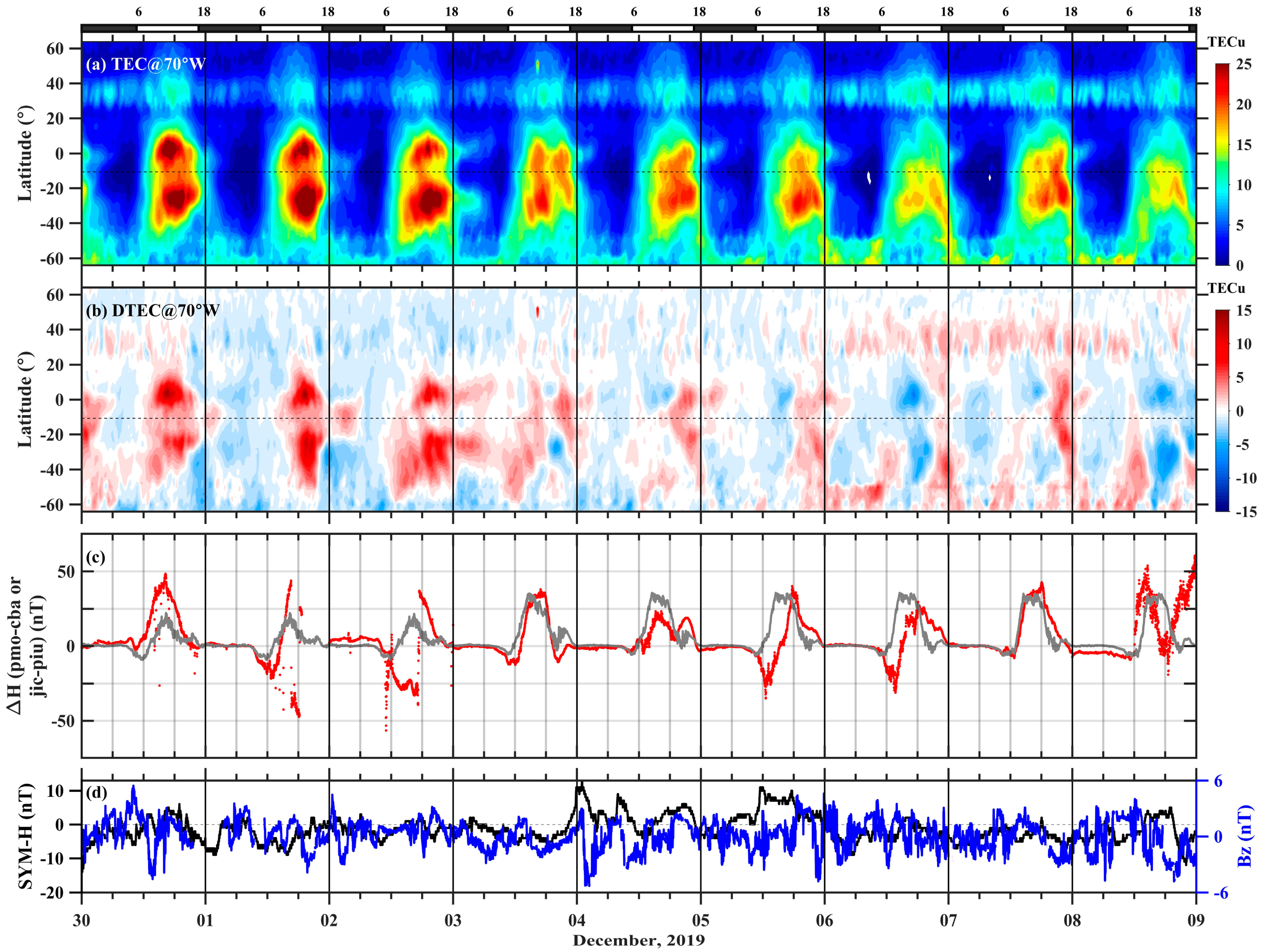
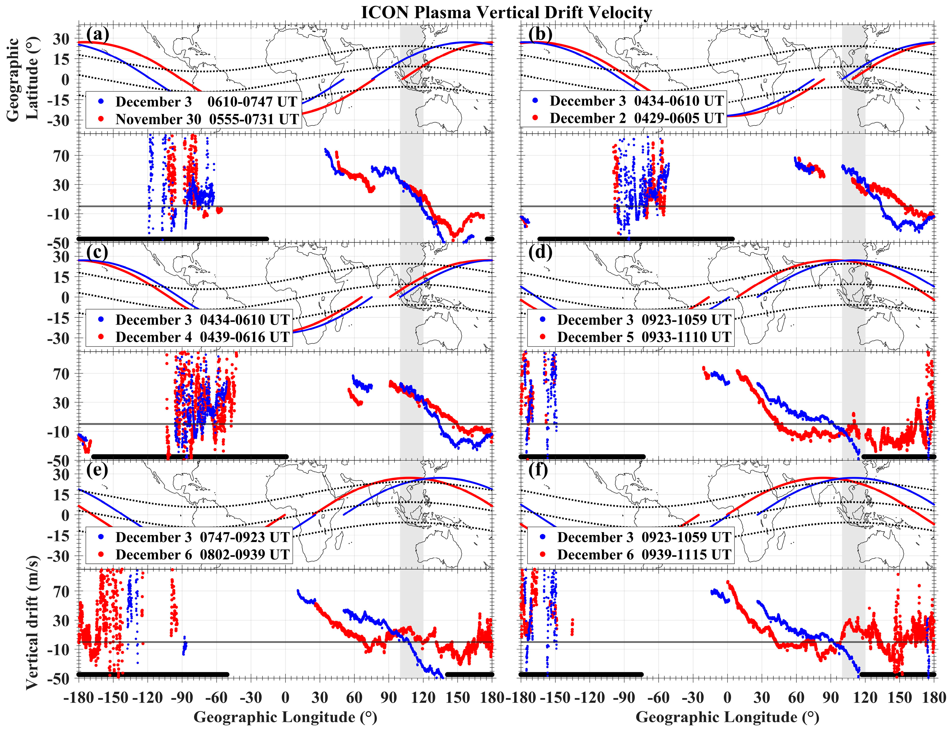
3.2. Ionospheric Variations (dTEC), ΔH, and Vertical Plasma Drift Velocity from ICON

At an altitude of about 95 km, the tidal winds were strongly variable at mid/low-latitudes during the period (see Kuai et al. [1] for details). The notably changing tides in the mesosphere and lower thermosphere regions are likely to affect the ionospheric E-region dynamo. The changing tides may also lead to changes in the electric fields [39,40,41,42]. This, in turn, leads to the changes in ionospheric electron density/TEC. Figure 2 displays the variations in TEC/DTEC/ΔH/SYM-H/IMF Bz in the American sector during the period from 30 November to 8 December 2019 (from Kuai et al. [1]). As seen in Figure 2b,c, TEC significantly enhanced during the daytime from 30 November to 2 December, but the ΔH decreased during this time. TEC significantly increased, especially from 1200 UT to 1800 UT on 2 December, but ΔH clearly decreased. It can also be noted that ΔH decreased clearly at 1200–1800 UT on 5 and 6 December, but the variations in TEC were not significant. The changes in TEC and ΔH are inconsistent in this sector during these times.
Considering the limitations of using only geomagnetic data to reflect the electric field, we used the vertical plasma drift data from ICON to further explore the effects of the electric fields in this case. The gray areas in Figure 3 show the variations in the satellite orbits and corresponding vertical plasma drift velocities from ICON in the American sector. The blue color represents the reference day (3 December 2019). The dashed lines represent the magnetic equator and ±15° magnetic latitudes.
As displayed in the gray part of Figure 3a, it can be found that the vertical drift velocities increased at ±15° magnetic latitudes and 50–80°W longitudes in the American sector at ~1400 UT on 1 December, compared with 3 December. Meanwhile, TEC showed a positive phase, but ΔH values were decreasing (see Figure 2b,c, ~1400 UT on 1 December). As depicted in the gray parts of Figure 3b,c, it can be seen that the vertical drift velocities significantly increased at ~1540 UT on 2 December compared with 3 December, with the largest change from about 14 m/s to 46 m/s. At the same time, the TEC obviously enhanced, but ΔH remarkably declined (see Figure 2b,c, ~1540 UT on 2 December).
In the American sector, the variations in TEC were consistent with the changes in vertical plasma drift velocities. The enhanced eastward electric fields produced the upward vertical E×B drifts. The upward vertical E × B drifts pushed the plasma upward and caused vertical plasma drift velocities to increase. We speculate that the enhanced eastward electric fields are the cause of the enhancement of TEC from 1 December to 2 December.
A similar situation also occurred in the Asian–Australian sector. Figure 4 gives the variations in TEC/DTEC/ΔH in the Asian–Australian sector from 30 November to 8 December, and the geomagnetic indexes were also marked (from Kuai et al. [1]). As depicted in Figure 4b, the TEC showed positive phases at ~0600 UT on 30 November and ~1000 UT on 5 December, especially at 0600–1200 UT on 6 December, when the TEC obviously enhanced. However, it can be seen from Figure 4c that ΔH almost did not change during these time periods. At ~0500 UT on 4 December, ΔH changed significantly, while TEC only changed slightly. The disturbances in TEC are inconsistent with the changes in ΔH from 4 to 6 December.
We also focus on the changing vertical plasma drift velocities during these days in the Asian–Australian sector. Figure 5 plots the satellite orbits and corresponding vertical plasma drift velocities from ICON. The blue color denotes the reference day (3 December 2019). The geographic longitude range of the gray areas is 100°–120°E. Similar to the phenomena in the American sector, the TEC changes are consistent with the changes in the vertical plasma drift velocities at ±15° magnetic latitudes and 100–120°E longitudes in the Asian–Australian sector when comparing Figure 4b and the gray areas in Figure 5. But the changes in the vertical plasma drift velocities and ΔH are inconsistent. In particular, the variations in the vertical plasma drift velocities are strong, with a significant enhancement, which fits well with the changes in TEC at ~0830 UT and ~1010 UT on 6 December (Figure 5e,f) in the Asian–Australian sector. Likewise, the enhanced eastward electric fields may have led to the enhanced TEC in this sector during this event.
It can be seen that the variations in the vertical plasma drift velocities and ΔH are quite different in the two sectors. ΔH provides a direct measurement of the daytime electrojet flow, which in turn can indicate the magnitude of the vertical E × B drift velocity in the F-region ionosphere. The relationship between the ΔH and E × B drift value varies at different longitudes, solar activity levels, seasons, and so on [29]. In other words, the relationship between ΔH and the electric field does not show a strict correlation. Furthermore, for the work in Kuai et al. [1], the selections of the stations used to obtain the ΔH are not particularly suitable due to the incompleteness of the H data during this event. These seem to explain the inconsistency between the ΔH changes and the vertical plasma drift velocity variations in the present event.
To further analyze the electrodynamic process of this event, we plotted the variations in foF2 and hmF2 using the Lowell DPS-4D ionosonde data at Sanya, considering that the ICON orbits of several cases shown in the gray areas of Figure 5 were just near Sanya in geographical position. Figure 6 displays the temporal series of foF2 (a) and hmF2 (b) at Sanya (109.6°E, 18.3°N) during 30 November–8 December. The gray lines show the reference values derived from the 27-day running median values of foF2 and hmF2. The effects of solar rotation can be effectively removed by the 27-day running median [43]. The gray areas denote the time ranges of 0930–1100 UT on 5 December and 0800–1100 UT on 6 December, respectively. As illustrated in the gray areas of Figure 6, foF2 and hmF2 increased at 0930–1100 UT on 5 December and significantly enhanced at 0800–1100 UT on 6 December.
The upward vertical E × B drifts push the plasma upward. The increases in hmF2 indicate the upward vertical E × B drifts, which are consistent with the enhancements in vertical plasma drift velocities from ICON. In other words, the eastward electric fields led to the increase in hmF2 and foF2.
In summary, the enhanced eastward electric fields may be causing changes in hmF2 and TEC at low latitudes in both the American and the Asian–Australian sectors during this case. Another important point is that sometimes the geomagnetic ΔH data could not indicate the variations in the electric fields in the F-region ionosphere, such as this GQT in our case.

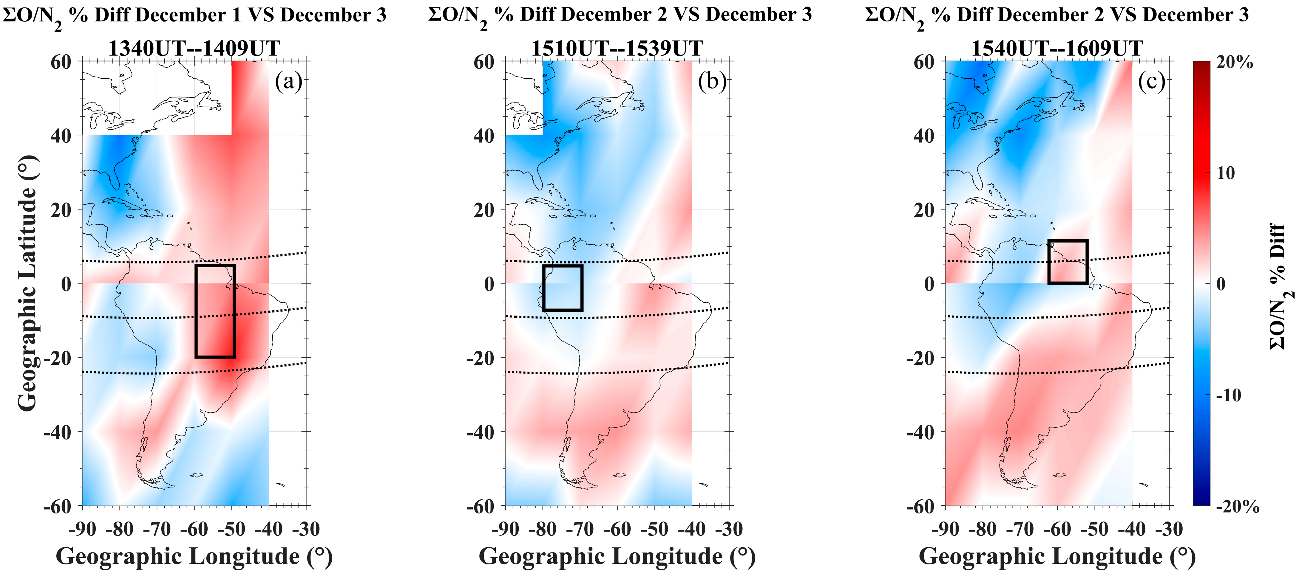
3.3. Neutral Compositions ∑O/N2 from GOLD

During this GQT, the IMF By index oscillated between −5 and 5 nT. As shown in Figure 1, |By| > |Bz| had a total length of more than 37 h from 30 November to 2 December. By dominated the IMF conditions for more than half of the three days. The By dominant condition could enhance the variations in neutral composition during geomagnetically quiet conditions [26]. The neutral composition changes could also affect variations in TEC. According to incomplete data, Kuai et al. [1] observed weak changes in ∑O/N2 observed by TIMED/GUVI at mid/low-latitudes and they could only consider that changes in ∑O/N2 had less impact at mid/low-latitudes during this period.
To further research the variations in neutral composition, ∑O/N2 data from GOLD were used in this work. Note that the GOLD data focus on the American sector. Figure 7 exhibits a temporal series of ∑O/N2 from GOLD in the geographic longitude 60°–80°W. The red, blue, yellow, and gray colors indicate 30 November and 1 to 3 December, respectively. The gray color shows the reference values of ∑O/N2 on 3 December.
As seen in Figure 7, the red color represents variations in ∑O/N2 on 30 November. The ∑O/N2 were significantly stronger at both 30°–40°N and 30°–40°S and enhanced at both 50°–60°N and 10°S–10°N on 30 November compared to the reference day. The ∑O/N2 decreased at 1000–1500 UT and 50°–60°S latitudes. The variations in [O/N2] were stronger at mid-latitude and weaker at low-latitude, and showed a clear hemispheric asymmetry.
According to the classical photoionization theory, compositional effects affect the generation and recombination of electrons in the ionosphere, which in turn influences the ionospheric TEC. Generally, if other factors are not considered, when ΣO/N2 increases, the electron density and TEC are also enhanced, and vice versa. The ∑O/N2 distributions of the cases shown in Figure 3 are presented. Figure 8 depicts the percentage difference in ∑O/N2 from GOLD in the coordinates of the geographic longitude and latitude at 1340–1409 UT on 1 December (a), 1510–1539 UT (b), and 1540–1609 UT (c) on 2 December. The black rectangular areas in Figure 8a–c indicate where the ICON orbits pass through in the gray areas of Figure 3a–c. The percentage differences of ∑O/N2 were obtained by using the ∑O/N2 data on December 3 as the reference values. The ∑O/N2 measured by GOLD had unrealistically higher values near 0–20°S, which led to discontinuities in the ΣO/N2 data around the equator [37]. The ΣO/N2 data were gridded by 10° × 20° (longitude × latitude) bins in this work. The median ΣO/N2 value of each bin was derived, thus reducing errors and removing small-scale disturbances. The percentage variations in ΣO/N2 compared to the reference value further reduced the error of the GOLD measurement at 0–20°S. In our case, this error can be considered to be effectively eliminated.
As illustrated in the black rectangular areas of Figure 2 and Figure 8a,c, ∑O/N2 and TEC were both increased. As shown in the black rectangular area of Figure 8b, ∑O/N2 decreased, but TEC was enhanced. In order to demonstrate the continuous percentage variations in ΣO/N2, Figure S1 in the Supplementary Material gives the ΣO/N2 percentage deviation evolutions at 1140–2000 UT on 1 and 2 December 2019, compared to December 3. From the Figure S1a, it can be seen that ΣO/N2 increased at 1140–1433 UT on 1 December in the black rectangular area. As can be seen in the Figure S1b, ΣO/N2 decreased at 1410–1639 UT on 2 December in the black rectangular region. It can be observed in the black rectangular region in Figure S1c that ΣO/N2 enhanced at 1240–1933 UT on 2 December. It can be seen that the changes in ∑O/N2 were not exactly consistent with the variations in TEC (Figure 2b). Relatively speaking, the disturbances in neutral composition should make a minor contribution to the changes in TEC during these cases, compared with the electric fields.
The changed ionospheric electric fields caused by the tidal winds and the thermospheric compositional variations due to geomagnetic forcing and IMF By play important roles in the ionospheric day-to-day variations [1,25,26]. In addition, could there be any other mechanisms during these periods? The complex processes of all the factors are still not clear enough. More numerical simulations with models that include both lower atmospheric forcing and geomagnetic forcing will be carried out to further investigate day-to-day ionospheric variations.

4. Conclusions

In this work, we further analyzed the ionospheric variations at mid/low-latitudes during the GQT from 30 November to 8 December 2019, utilizing vertical plasma drift data from ICON and ∑O/N2 data from GOLD. The main conclusions are summarized below:
  • There were noticeable changes in vertical drift velocities from ICON at low latitudes. In the American sector, the vertical drift velocities showed significant enhancements on 1 and 2 December. For the Asian–Australian sector, the main characteristic of the vertical drift velocities was the significant increase during the daytime on 6 December.
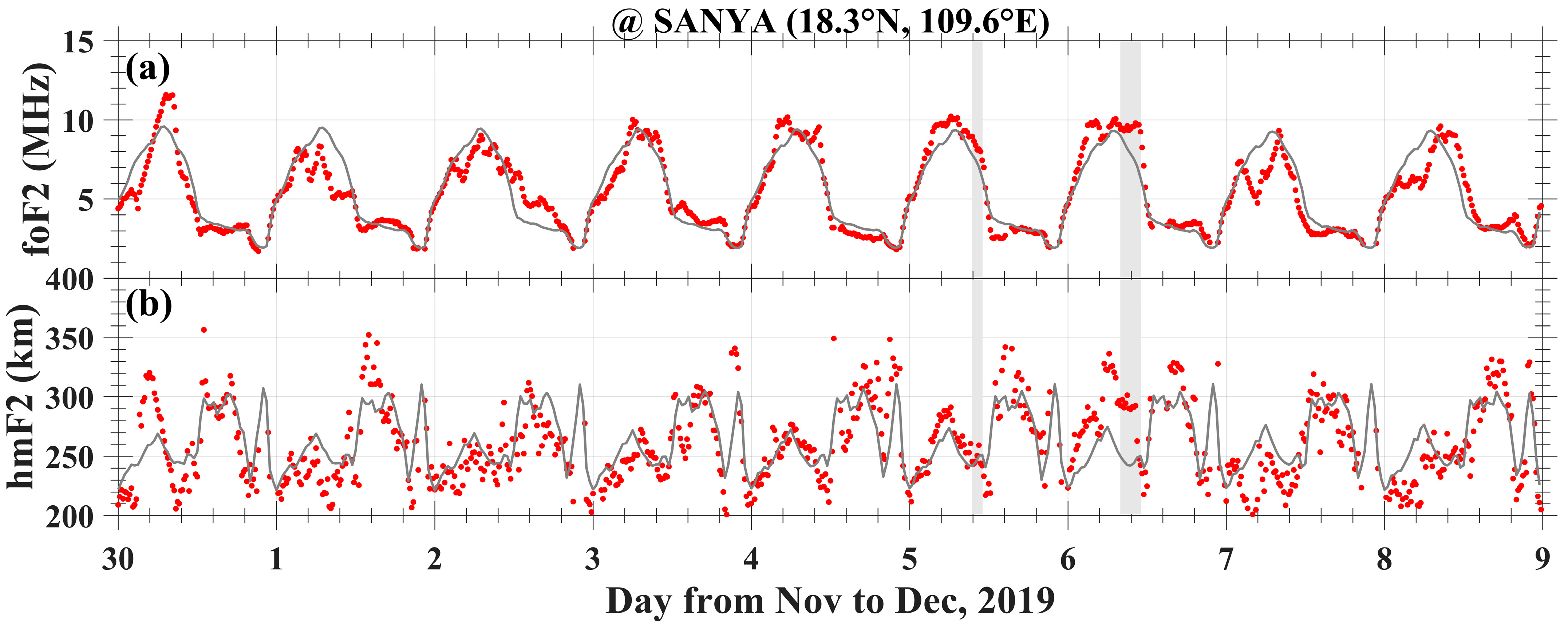
  • The foF2 and hmF2 had prominent variations at Sanya. In particular, both showed significant increases on 6 December. This indicates the presence of an upward E × B drift, which is consistent with the change in vertical drift velocities from ICON.
  • The changes in TEC and vertical drift velocities were consistent at low latitudes. The changes in zonal electric fields should be the main cause of the change in TEC in both the American and the Asian–Australian sectors.
  • The variations in ΔH did not perfectly correspond to the changes in the E × B drift in this case. In other words, sometimes the geomagnetic data ΔH did not indicate variations in the electric fields in the F-region ionosphere, such as the GQT in our case.
  • ∑O/N2 from GOLD showed strong enhancements at mid-latitudes on 30 November in the American sector. And the changes in ∑O/N2 showed a hemispheric asymmetry. The changes in the neutral compositions did not exactly coincide with the changes in TEC, and it is speculated that the neutral compositions should make a minor contribution to the changes in TEC during this event, compared with the electric fields.

Supplementary Materials

The following supporting information can be downloaded at: https://www.mdpi.com/article/10.3390/rs15235591/s1, Figure S1. Variations in the percentage deviations in ΣO/N2 from GOLD in the American sector during 1140–2000 UT on 1 and 2 December, compared to 3 December 2019. The black rectangular areas in Figures S1a, S1b, and S1c indicate the black rectangular areas of Figure 8a–c.

Author Contributions

Conceptualization, J.K., H.S., J.Z. and L.L.; methodology, J.K., H.S., J.Z., L.L., R.Z., Q.L. and L.H.; software, H.S., J.K., and J.Z.; validation, J.K., J.Z., L.L., R.Z., Q.L. and L.H.; formal analysis, J.K., L.L. and J.Z.; investigation, H.S., J.K., J.Z., L.L. and L.H.; resources, H.S., J.K., J.Z., L.L. and L.H.; data curation, H.S. and J.K.; writing—original draft preparation, H.S. and J.K.; writing—review and editing, H.S., J.K., J.Z., L.L., R.Z., Q.L. and L.H.; visualization, H.S., J.K., J.Z. and L.L.; supervision, J.K., J.Z., L.L. and L.H.; project administration, J.K., J.Z., L.L. and L.H.; funding acquisition, J.K., J.Z., L.L., R.Z. and Q.L. All authors have read and agreed to the published version of the manuscript.

Funding

This research was funded by the National Natural Science Foundation of China, grant numbers 42030202, 41804153, 42374181, 41804150, 42174204, 42104147; the Natural Science Foundation of Jiangsu Province, grant number BK20180445; the seventh Young Elite Scientists Sponsorship Program of the China Association for Science and Technology, grant number 2021QNRC001; Shanghai Aerospace Science and Technology Innovation Fund, grant number SAST2021-075; Key Laboratory Stability Support Fund, grant number HTKJ2022KL504017; the Fundamental Research Funds for the Central Universities, Nanjing University of Aeronautics and Astronautics, grant number NP2022449; Guangdong Basic and Applied Basic Research Foundation, grant number 2021A1515011216, 2020A1515110242; the Opening Funding of the Chinese Academy of Sciences dedicated for the Chinese Meridian Project; and the Open Research Project of Large Research Infrastructures of CAS—“Study on the interaction between low/mid-latitude atmosphere and ionosphere based on the Chinese Meridian Project”.

Data Availability Statement

The solar wind data were obtained from the OMNIWeb interface at http://omniweb.gsfc.nasa.gov, accessed on 18 November 2023. The ICON data are available at the website of https://cdaweb.gsfc.nasa.gov/pub/data/icon, https://icon.ssl.berkeley.edu/Data, accessed on 2 November 2023. GOLD data presented in this paper can be accessed at the GOLD Science Data Center (http://gold.cs.ucf.edu/search/), accessed on 2 November 2023.

Acknowledgments

We are grateful to the broader ICON team. We thank NASA/GOLD and the mission science team. The foF2 and hmF2 data were recorded at Sanya, which is under the operation of the Beijing National Observatory of Space Environment. We acknowledge the use of data from the Chinese Meridian Project.

Conflicts of Interest

The authors declare no conflict of interest.

References

  1. Kuai, J.; Li, Q.; Zhong, J.; Zhou, X.; Liu, L.; Yoshikawa, A.; Hu, L.; Xie, H.; Huang, C.; Yu, X.; et al. The ionosphere at middle and low latitudes under geomagnetic quiet time of December 2019. J. Geophys. Res. Space Phys. 2021, 126, e2020JA028964. [Google Scholar] [CrossRef]
  2. Kawamura, S.; Balan, N.; Otsuka, Y.; Fukao, S. Annual and semiannual variations of the midlatitude ionosphere under low solar activity. J. Geophys. Res. 2002, 107, 1166. [Google Scholar] [CrossRef]
  3. Liu, H.; Stolle, C.; Förster, M.; Watanabe, S. Solar activity dependence of the electron density in the equatorial anomaly regions observed by CHAMP. J. Geophys. Res. 2007, 112, A11311. [Google Scholar] [CrossRef]
  4. Zhao, B.; Hao, Y. Ionospheric and geomagnetic disturbances caused by the 2008 Wenchuan earthquake: A revisit. J. Geophys. Res. Space Phys. 2015, 120, 5758–5777. [Google Scholar] [CrossRef]
  5. Bolaji, O.S.; Adebiyi, S.J.; Fashae, J.B. Characterization of ionospheric irregularities at different longitudes during quiet and disturbed geomagnetic conditions. J. Atmos. Sol.-Terr. Phys. 2019, 182, 93–100. [Google Scholar] [CrossRef]
  6. Wang, W.; Burns, A.G.; Liu, J. Upper Thermospheric Winds. In Upper Atmosphere Dynamics and Energetics; Wang, W., Zhang, Y., Paxton, L.J., Eds.; American Geophysical Union: Washington, DC, USA, 2021. [Google Scholar] [CrossRef]
  7. Schmölter, E.; von Savigny, C. Solar activity driven 27-day signatures in ionospheric electron and molecular oxygen densities. J. Geophys. Res. Space Phys. 2022, 127, e2022JA030671. [Google Scholar] [CrossRef]
  8. Appleton, E.V.; Ingram, L.J. Magnetic storms and upper-atmospheric ionisation. Nature 1935, 136, 548–549. [Google Scholar] [CrossRef]
  9. Galushko, V.G.; Paznukhov, V.V.; Sopin, A.A.; Yampolski, Y.M. Statistics of ionospheric disturbances over the Antarctic Peninsula as derived from TEC measurements. J. Geophys. Res. Space Phys. 2016, 121, 3395–3409. [Google Scholar] [CrossRef]
  10. Prölss, G.W. Ionospheric storms at mid-latitude: A short review. In Midlatitude Ionospheric Dynamics and Disturbances; Geophysical Monograph, Series; Kintnet, P.M., Coster, A.J., Fuller-Rowell, T., Mannucci, A.J., Mendillo, M., Heelis, R., Eds.; American Geophysical Union: Washington, DC, USA, 2008; Volume 181, pp. 9–24. [Google Scholar] [CrossRef]
  11. Forbes, J.M.; Palo, S.E.; Zhang, X. Variability of the ionosphere. J. Atmos. Sol.-Terr. Phys. 2000, 62, 685–693. [Google Scholar] [CrossRef]
  12. Rishbeth, H.; Mendillo, M. Patterns of F2-layer variability. J. Atmos. Sol.-Terr. Phys. 2001, 63, 1661–1680. [Google Scholar] [CrossRef]
  13. Zhang, S.-R.; Holt, J.M. Ionospheric variability from an incoherent scatter radar long-duration experiment at Millstone Hill. J. Geophys. Res. 2008, 113, A03310. [Google Scholar] [CrossRef]
  14. Depuev, V.; Depueva, A.; Leshchinskaya, T.Y. Mechanism of formation of Q-disturbances in the F2 region of the equatorial ionosphere. Geomagn. Aeron. 2008, 48, 89–97. [Google Scholar] [CrossRef]
  15. Zhou, X.; Yue, X.; Liu, H.-L.; Lu, X.; Wu, H.; Zhao, X.; He, J. A comparative study of ionospheric day-to-day variability over Wuhan based on ionosonde measurements and model simulations. J. Geophys. Res. Space Phys. 2021, 126, e2020JA028589. [Google Scholar] [CrossRef]
  16. Klenzing, J.; Burrell, A.G.; Heelis, R.A.; Huba, J.D.; Pfaff, R.; Simões, F. Exploring the role of ionospheric drivers during the extreme solar minimum of 2008. Ann. Geophys. 2013, 31, 2147–2156. [Google Scholar] [CrossRef]
  17. Huang, F.; Lei, J.; Dou, X. Daytime ionospheric longitudinal gradients seen in the observations from a regional BeiDou GEO receiver network. J. Geophys. Res. Space Phys. 2017, 122, 6552–6561. [Google Scholar] [CrossRef]
  18. Liu, G.; England, S.L.; Immel, T.J.; Frey, H.U.; Mannucci, A.J.; Mitchell, N.J. A comprehensive survey of atmospheric quasi 3 day planetary-scale waves and their impacts on the day-to-day variations of the equatorial ionosphere. J. Geophys. Res. Space Phys. 2015, 120, 2979–2992. [Google Scholar] [CrossRef]
  19. Cai, X.; Burns, A.G.; Wang, W.; Coster, A.; Qian, L.; Liu, J.; Solomon, S.C.; Eastes, R.W.; Daniell, R.E.; McClintock, W.E. Comparison of GOLD nighttime measurements with total electron content: Preliminary results. J. Geophys. Res. Space Phys. 2020, 125, e2019JA027767. [Google Scholar] [CrossRef]
  20. Cai, X.; Burns, A.G.; Wang, W.; Qian, L.; Solomon, S.C.; Eastes, R.W.; Pedatella, N.; Daniell, R.E.; McClintock, W.E. The two-dimensional evolution of thermospheric ∑O/N2 response to weak geomagnetic activity during solar-minimum observed by GOLD. Geophys. Res. Lett. 2020, 47, e2020GL088838. [Google Scholar] [CrossRef]
  21. Liu, J.; Zhang, D.; Hao, Y.; Xiao, Z. Multi-instrumental observations of the quasi-16-day variations from the lower thermosphere to the topside ionosphere in the low-latitude eastern Asian sector during the 2017 sudden stratospheric warming event. J. Geophys. Res. Space Phys. 2020, 125, e2019JA027505. [Google Scholar] [CrossRef]
  22. Yamazaki, Y.; Häusler, K.; Wild, J.A. Day-to-day variability of midlatitude ionospheric currents due to magnetospheric and lower atmospheric forcing. J. Geophys. Res. Space Phys. 2016, 121, 7067–7086. [Google Scholar] [CrossRef]
  23. Xiong, B.; Wang, Y.; Li, Y.; Zhao, B.; Yu, Y.; Ren, Z.; Hu, L.; Sun, W.; Wu, Z. Anomalous disturbance of the ionosphere in the East Asia region during the geomagnetically quiet day on 1 November 2016. J. Geophys. Res. Space Phys. 2023, 128, e2022JA030905. [Google Scholar] [CrossRef]
  24. Liu, L.; Ding, Z.; Zhang, R.; Chen, Y.; Le, H.; Zhang, H.; Li, G.; Wu, J.; Wan, W. A Case Study of the Enhancements in Ionospheric Electron Density and Its Longitudinal Gradient at Chinese Low Latitudes. J. Geophys. Res. Space Phys. 2020, 124, e2019JA027751. [Google Scholar] [CrossRef]
  25. Cai, X.; Burns, A.G.; Wang, W.; Qian, L.; Pedatella, N.; Coster, A.; Zhang, S.; Solomon, S.C.; Eastes, R.W.; Daniell, R.E.; et al. Variations in Thermosphere Composition and Ionosphere Total Electron Content Under “Geomagnetically Quiet” Conditions at Solar-Minimum. Geophys. Res. Lett. 2021, 48, e2021GL093300. [Google Scholar] [CrossRef]
  26. Cai, X.; Wang, W.; Burns, A.; Qian, L.; Eastes, R.W. The Effects of IMF By on the Middle Thermosphere During a Geomag-netically “Quiet” Period at Solar Minimum. J. Geophys. Res. Space Phys. 2022, 127, e2021JA029816. [Google Scholar] [CrossRef]
  27. McComas, D.J.; Bame, S.J.; Barker, P.; Feldman, W.C.; Phillips, J.L.; Riley, P.; Griffee, J.W. Solar Wind Electron Proton Alpha Monitor (SWEPAM) for the Advanced Composition Explorer. Space Sci. Rev. 1998, 86, 563–612. [Google Scholar] [CrossRef]
  28. Wanliss, J.A.; Showalter, K.M. High-Resolution Global Storm Index: Dst versus SYM-H. J. Geophys. Res. Space Phys. 2006, 111, e2005JA011034. [Google Scholar] [CrossRef]
  29. Anderson, D.; Anghel, A.; Yumoto, K.; Ishitsuka, M.; Kudeki, E. Estimating Daytime Vertical E×B Drift Velocities in the Equatorial F-region Using Ground-based Magnetometer Observations. Geophys. Res. Lett. 2002, 29, 37-1–37-4. [Google Scholar] [CrossRef]
  30. Rideout, W.; Coster, A. Automated GPS Processing for Global Total Electron Content Data. GPS Solut. 2006, 10, 219–228. [Google Scholar] [CrossRef]
  31. Heelis, R.A.; Stoneback, R.A.; Perdue, M.D.; Depew, M.D.; Morgan, W.A.; Mankey, M.W.; Lippincott, C.R.; Harmon, L.L.; Holt, B.J. Ion Velocity Measurements for the Ionospheric Connections Explorer. Space Sci. Rev. 2017, 212, 615–629. [Google Scholar] [CrossRef]
  32. Immel, T.J.; England, S.L.; Mende, S.B.; Heelis, R.A.; Englert, C.R.; Edelstein, J.; Frey, H.U.; Korpela, E.J.; Taylor, E.R.; Craig, W.W.; et al. The Ionospheric Connection Explorer Mission: Mission Goals and Design. Space Sci. Rev. 2017, 214, 13. [Google Scholar] [CrossRef]
  33. Hysell, D.L.; Kirchman, A.; Harding, B.J.; Heelis, R.A.; England, S.L. Forecasting Equatorial Ionospheric Convective Instability With ICON Satellite Measurements. Space Weather 2023, 21, e2023SW003427. [Google Scholar] [CrossRef]
  34. Zhang, R.; Liu, L.; Ma, H.; Chen, Y.; Le, H. ICON Observations of Equatorial Ionospheric Vertical ExB and Field-Aligned Plasma Drifts During the 2020–2021 SSW. Geophys. Res. Lett. 2022, 49, e2022GL099238. [Google Scholar] [CrossRef]
  35. Eastes, R.W.; McClintock, W.E.; Burns, A.G.; Anderson, D.N.; Andersson, L.; Codrescu, M.; Correira, J.T.; Daniell, R.E.; England, S.L.; Evans, J.S.; et al. The Global-Scale Observations of the Limb and Disk (GOLD) Mission. Space Sci. Rev. 2017, 212, 383–408. [Google Scholar] [CrossRef]
  36. Eastes, R.W.; McClintock, W.E.; Burns, A.G.; Anderson, D.N.; Andersson, L.; Aryal, S.; Budzien, S.A.; Cai, X.; Codrescu, M.V.; Correira, J.T.; et al. Initial Observations by the GOLD Mission. JGR Space Phys. 2020, 125, e2020JA027823. [Google Scholar] [CrossRef]
  37. Correira, J.; Evans, J.S.; Lumpe, J.D.; Krywonos, A.; Daniell, R.; Veibell, V.; McClintock, W.E.; Eastes, R.W. Thermospheric Composition and Solar EUV Flux From the Global-Scale Observations of the Limb and Disk (GOLD) Mission. J. Geophys. Res. Space Phys. 2021, 126, e2021JA029517. [Google Scholar] [CrossRef]
  38. Huang, X.; Reinisch, B.W. Vertical Electron Density Profiles from the Digisonde Network. Adv. Space Res. 1996, 18, 121–129. [Google Scholar] [CrossRef]
  39. Wan, W.; Liu, L.; Pi, X.; Zhang, M.-L.; Ning, B.; Xiong, J.; Ding, F. Wavenumber-4 Patterns of the Total Electron Content over the Low Latitude Ionosphere. Geophys. Res. Lett. 2008, 35, 2008GL033755. [Google Scholar] [CrossRef]
  40. England, S.L.; Immel, T.J.; Sagawa, E.; Henderson, S.B.; Hagan, M.E.; Mende, S.B.; Frey, H.U.; Swenson, C.M.; Paxton, L.J. Effect of Atmospheric Tides on the Morphology of the Quiet Time, Postsunset Equatorial Ionospheric Anomaly. J. Geophys. Res. 2006, 111, 2006JA011795. [Google Scholar] [CrossRef]
  41. Liu, J.; Wang, W.; Burns, A.; Solomon, S.C.; Zhang, S.; Zhang, Y.; Huang, C. Relative Importance of Horizontal and Vertical Transports to the Formation of Ionospheric Storm-enhanced Density and Polar Tongue of Ionization. JGR Space Phys. 2016, 121, 8121–8133. [Google Scholar] [CrossRef]
  42. Millward, G.H.; Müller-Wodarg, I.C.F.; Aylward, A.D.; Fuller-Rowell, T.J.; Richmond, A.D.; Moffett, R.J. An Investigation into the Influence of Tidal Forcing on F Region Equatorial Vertical Ion Drift Using a Global Ionosphere-thermosphere Model with Coupled Electrodynamics. J. Geophys. Res. 2001, 106, 24733–24744. [Google Scholar] [CrossRef]
  43. Kuai, J.; Liu, L.; Liu, J.; Zhao, B.; Chen, Y.; Le, H.; Wan, W. The Long-duration Positive Storm Effects in the Equatorial Ionosphere over Jicamarca. J. Geophys. Res. Space Phys. 2015, 120, 1311–1324. [Google Scholar] [CrossRef]
Figure 1. Variations in F10.7 index, the solar wind speed velocity (VSW, km/s), the interplanetary magnetic field (IMF), Bz and By components (nT), Ey (mV/m), SYM-H index (nT), and Kp index from 30 November to 8 December 2019 (the days of year are 334 to 342).
Remotesensing 15 05591 g001
Figure 2. Geographic longitude and UT distribution of TEC (a) and the deviations in TEC (DTEC) (b) in the American sector. (c) The changes in ΔH. (d) The SYM-H and IMF Bz index (blue line). The bar at the upper edge indicates the local time. The gray curve in Figure 2c indicates reference values derived from the 27-day running median value of ΔH. Reprinted with permission from Kuai et al. [1]. Copyright 2021 American Geophysical Union.
Remotesensing 15 05591 g002
Figure 3. Variations in the satellite orbits and corresponding vertical plasma drift velocities from ICON at (a) ~1225–1402 UT on December 1, (b) ~1407–1543 UT on December 2, and (c) ~1543–1720 UT on December 2, respectively. The blue color represents the reference day (3 December 2019). The dashed lines represent ±15° magnetic latitudes and the magnetic equator. The legends mark the corresponding time (day and UT) of the ICON orbits. The geographic longitude range of the gray areas is 50°–80°W. The black bars indicate the period from 1800–0600 LT on the night side.
Remotesensing 15 05591 g003
Figure 4. (a) Geographic longitude and UT distribution of TEC and (b) the deviations in TEC (DTEC) in the Asian–Australian sector. (c) The changes in ΔH. (d) The SYM-H and IMF Bz index (blue line). The 1800–0600 LT period for the night side is indicated by the bar at the top of this figure. The quiet-time reference values, derived from the 27-day running median value of ΔH, are shown by the gray curve in Figure 4c. Reprinted with permission from Kuai et al. [1]. Copyright 2021 American Geophysical Union.
Remotesensing 15 05591 g004
Figure 5. Variations in the satellite orbits and corresponding vertical plasma drift velocities from ICON at (a) ~0555–0731 UT on November 30, (b) ~0429–0605 UT on December 2, (c) ~0439–0616 UT on December 4, (d) ~0933–1110 UT on December 5, (e) ~0802–0939 UT and (f) ~0936–1115 UT on December 6, respectively. The blue color denotes the reference day (3 December 2019). The dashed lines represent ±15° magnetic latitudes and the magnetic equator. The legends mark the corresponding time (day and UT) of the ICON orbits. The geographic longitude range of the gray areas is 100°–120°E. The black bars indicate the period from 1800–0600 LT on the night side.
Remotesensing 15 05591 g005
Figure 6. Temporal series of foF2 (a) and hmF2 (b) over Sanya (109.6°E, 18.3°N) during 30 November–8 December 2019. The red dots denote the observed foF2 and hmF2 and the gray curves show the reference values obtained by using the 27-day running median values of foF2 and hmF2. The gray areas denote the time ranges of 0930–1100 UT on 5 December and 0800–1100 UT on 6 December, respectively.
Remotesensing 15 05591 g006
Figure 7. Temporal series of ∑O/N2 from GOLD in the geographic longitude 60°–80°W for geographic latitudes (a) 50°–60°N, (b) 30°–40°N, (c) 10°S–10°N, (d) 30°–40°S, and (e) 50°–60°S, respectively. The red, blue, yellow, and gray colors indicate 30 November and 1 to 3 December, respectively. The gray color shows the reference values of ∑O/N2 on 3 December. The legends mark the corresponding geographic latitudes of ∑O/N2.
Remotesensing 15 05591 g007
Figure 8. The percentage difference in ∑O/N2 from GOLD in the coordinates of the geographic longitude and latitude at 1340–1409 UT on 1 December (a), 1510–1539 UT (b), and 1540–1609 UT (c) on 2 December. The black rectangular areas in Figure 8a–c indicate where ICON orbits pass through in the gray area of Figure 3a–c. The percentage difference in ∑O/N2 was obtained by using the ∑O/N2 data on 3 December as the reference value. The black dotted lines of the geomagnetic latitudes at 0° and ±15° are plotted for reference.
Remotesensing 15 05591 g008
Disclaimer/Publisher’s Note: The statements, opinions and data contained in all publications are solely those of the individual author(s) and contributor(s) and not of MDPI and/or the editor(s). MDPI and/or the editor(s) disclaim responsibility for any injury to people or property resulting from any ideas, methods, instructions or products referred to in the content.

