

Optimization of the Vertical Wavenumber for PolInSAR Inversion Performance Based on Numerical CRLB Analysis


College of Computer and Information Engineering, Nanjing Tech University, Nanjing 211816, China
*
Author to whom correspondence should be addressed.
Remote Sens. 2023, 15(22), 5321; https://doi.org/10.3390/rs15225321
Submission received: 30 August 2023
/
Revised: 6 November 2023
/
Accepted: 8 November 2023
/
Published: 10 November 2023
(This article belongs to the Special Issue SAR for Forest Mapping III)
Abstract
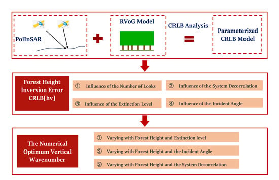
:A number of advanced SAR missions have been planned to launch, which can operate in fully polarimetric SAR interferometry mode to acquire structural parameters of global forests. Before the PolInSAR mission, the system configuration of vertical wavenumber must be carefully designed because it has a significant impact on the inversion performance. To minimize the estimation error of forest height caused by the system error from the future PolInSAR campaigns, it is valuable for us to optimize the vertical wavenumber. To quantitatively investigate the impact of on PolInSAR inversion performance, this paper proposes the optimization of based on the Cramér–Rao Lower Bound (CRLB) analysis. Extensive numerical CRLB simulations have been conducted to analyze the impact of several parameters, including extinction level, incident angle, and system decorrelation, etc., on the optimum . Finally, by minimizing the simulated CRLB, the numerical optimum maps are provided for the system engineers to easily design the system parameters.
1. Introduction
Since Polarimetric SAR interferometry (PolInSAR) has great potential in monitoring forest structures, several PolInSAR missions have been planned to launch, such as the Tandem-L mission [1,2] and the BIOMASS mission [3,4]. The advanced China L-band bistatic SAR mission LuTan-1 was successfully launched in 2022. Beyond the primary objective of generating a global digital elevation model (DEM), LuTan-1 can also configure full polarization mode to demonstrate the forest mapping and biomass inversion applications [5,6]. Single-baseline PolInSAR inversion usually requires a scattering model to separate the phase centers of the forest canopy and ground [7,8]. The commonly used random volume over ground (RVoG) scattering model proposed by Treuhaft et al. models the forest as a random particle layer located above a ground layer [9,10]. With the RVoG model, which relates the observed coherence with physical parameters, it is possible for us to invert the forest height [11,12,13,14,15].
As an indicator of the interferometer performance, the vertical wavenumber reflects the sensibility of the observations to physical parameters [16,17]. Different from InSAR application of DEM generation [18], the vertical wavenumber has a more complicated influence on PolInSAR forest height estimation [19,20,21]. Usually, an estimation accuracy on the order of 5–10% is required for forest height mapping [22]. Since vertical wavenumber has a notable influence on inversion performance, optimizing this parameter seems particularly important.
In 2005, by evaluating the interferometric phase error, Krieger et al. pointed out that several forest scenario parameters, different interferometric baselines, and temporal decorrelation will all affect the PolInSAR performance [23]. Cloude et al. proposed an approximate simple way to determine the vertical wavenumber based on geometric analysis of the coherence region [24]. Recently, Kugler et al. investigated the role of vertical wavenumber and found that each single vertical wavenumber is only suitable for specific height ranges [25].
To obtain a strict optimal solution, we have to resort to favorable mathematical tools. Fortunately, in 2011, Roueff et al. introduced the Cramér–Rao Lower Bound (CRLB) analysis into PolInSAR to evaluate the inversion performance [26]. Subsequently, Réfrégier and Roueff et al. reduced the independent parameters in the CRLB model, which makes the model easier to calculate [27]. Since the CRLB is independent of a specific estimation technique, it is useful to optimize the system configuration [28]. Several studies have initiated using the CRLB analysis to optimize the system configurations of PolInSAR, such as optimizing the polarization mode and baseline configuration [29,30].
Regarding the impact of on single-baseline PolInSAR inversion performance, no existing works have given the optimum baseline through quantitative analysis. Thanks to this error analysis tool, it is possible for us to realize the baseline optimization for PolInSAR forestry applications. In this paper, through the numerical CRLB simulations, we have optimized the PolInSAR inversion performance. The optimum changing with forest height and other important parameters have been numerically calculated. With the provided optimal baseline distribution map, the system engineers can easily and intuitively determine the PolInSAR system configuration.
The structure of this paper is organized as follows. Section 2 reviews the PolInSAR theory of forestry applications and formulates the CRLB of forest height for single-baseline PolInSAR. Section 3 analyzes the sensitivity of the vertical wavenumber, presents the CRLB analysis for inversion performance, and provides the contour map of the numerical optimum . Section 4 gives some discussion. Section 5 concludes the paper.
2. Materials and Methods
2.1. PolInSAR Preliminaries
2.1.1. The PolInSAR Measurements
Single-baseline PolInSAR measures the backscattered signals of the scene from two receiving antennas, which are space-shifted. And for each antenna , three different polarized backscattered signals can be obtained, which forms the two polarimetric scattering vectors as , where the superscript is the transpose operator. For the two observed scattering vectors and , the full information for the PolInSAR measurements is characterized by the following covariance matrix [11,12]
where the superscript is the Hermitian conjugate transpose operator, and the brackets is the statistical average. The polarimetric coherency matrices and involve the fully polarimetric information for each acquisition. The interferometric coherency matrix involves the polarimetric and interferometric relations between the two antenna acquisitions.
Due to the interferometric acquisition geometry of PolInSAR, the two acquisitions, and , are obtained at a given spatial baseline . As the acquisition geometry shown in Figure 1, the incident angle is , and represents the wavelength and the slant range, and is the perpendicular spatial baseline. The interferometric properties of the system can be characterized by the interferometric vertical wavenumber [16,17,18]
where the factor accounts for the acquisition mode, and are for the bistatic and monostatic acquisitions, respectively. The vertical wavenumber expresses the sensitivity of the interferometer, which has a critical impact on the related interferometric applications. For PolInSAR forest height estimation, the role of will be discussed later.
2.1.2. Forest RVoG Scattering Model
Single-baseline PolInSAR usually requires a scattering model to invert the forest parameters from the measurements. As an effective forest scattering model, the simple Random Volume over Ground (RVoG) model consists of two layers, which are the volume and ground layer [9,10]. The random volume is composed of randomly oriented particles, which are located above the ground layer of elevation , assuming that the vegetation height is , and the corresponding extinction level is denoted as . According to the forest RVoG scattering model, the PolInSAR observed coherency matrices in (1) are expressed as the contribution of the volume and the ground scattering as [26,31]
with
where and represent the volume polarimetric coherency matrix and ground polarimetric coherency matrix, respectively. Although a priori knowledge of scattering symmetry properties can reduce the unknown parameters in the two matrices and , it is seldom used in practice to improve the forest height estimation. Thus, we generally denote nine unknown real parameters in the matrix as
2.1.3. Modeling of PolInSAR Coherence
For any polarization vector , we can form two scalar images from the scattering vectors and and then compute the complex coherence. If we use the coherency matrices in (1) to express the complex coherence, we can get the general expression as [7,8]
The linear relation between the complex coherences and different polarizations on the complex plane can be utilized to perform the forest height inversion.
The observed complex coherence in the interferometric radar echoes involves several decorrelation processes. Considering the main decorrelation sources that affect the observed coherence, which is modeled as the multiplication of the following components [16,31]
The system decorrelation includes various kinds of decorrelation processes caused by the system and processing geometry. The temporal decorrelation contribution is very complicated, and we simply assume that . The volume decorrelation contribution is introduced by the ununiform forest scatterers. For forest scatterers, the vertical structure of the scatterers can be parameterized effectively by a two-layer RVoG model, which contains the volume and ground scattering contribution. Substituting the coherency matrices in (3) into (6) leads to the complex coherence equation for the forest RVoG scattering model [32]
where only the effective ground-to-volume scattering ratio is a function of polarization, which is expressed as
And is the polarization-independent volume integral equation given by
where expressed the exponential distribution of the vegetation layer
The volume-only coherence in (10) depends on four parameters, which are the vegetation height , the vertical wavenumber , the wave extinction , and the incidence angle .
2.2. CRLB for Single-Baseline PolInSAR
2.2.1. Formulation of CRLB
Cramér–Rao lower bound (CRLB) defines the theoretical boundary of the minimum estimation error. Since the CRLB does not rely on a particular estimation technique, we can use it to optimize the radar system parameters. For single-baseline PolInSAR inversion based on the parametrized RVoG model, we can formulate the CRLB of the forest height and the ground height , which has been previously presented in [26]. Assuming independent measurements of scattering vectors are available, then the covariance matrix with -look estimation can be obtained. Assuming an estimator denoted by , which estimates the height from the measured matrix . An unbiased estimator satisfies that the statistical expectation of the estimator equals the true vegetation height , that is
In that case, the performance of an unbiased estimator can be characterized by the variance of the estimator, and the statistical variance has the following minimal Cramér–Rao bound
According to the previous forest RVoG model, the polarimetric covariance matrix can be expressed by multiple parameters in (3)–(5), including , , , , , , and . Hence, the height estimator , along with its expectation, variance and the minimal variance are in general functions of these parameters, although no explicit expressions can be derived. Considering the forest height inversion process, the radar parameters and are known, and the scene-related parameters are to be estimated. So, the unknown parameters to be estimated can be defined by a parameter vector
It is thus clear that indicates the height estimation precision, which is a function of these 21 scalar unknown parameters in vector .
Among the parameter vector , the CRLB of the -th unknown parameter is defined as the element of the inverse of the Fisher information matrix , that is
The Fisher information matrix is a 21 × 21-dimensional matrix, and the element of the matrix is computed by
where is the number of looks, tr is the trace operator, and represents the covariance matrix parameterized by the unknown parameter vector . Finally, for the concerned forest height , the CRLB of is defined as the first element of the inverse of , which is given by
2.2.2. The Reduced RVoG Model
As previously shown in Section 2.1.2, the forest RVoG scattering model is determined with more than 20 parameters, which includes the forest parameters , , , , and , as well as the system configuration and . This many parameters makes it difficult to simulate and analyze all possible forest scenarios. However, the statistical invariance properties have shown that a few parameters can uniquely characterize the forest RVoG models, which possess the same polarimetric properties. And this group of models has identical CRLB values. Then, the reduced RVoG model with fewer parameters will greatly simplify the simulation and analysis of the forest scenarios.
Considering an initial RVoG model with forest parameters and a group of transformed RVoG models with transformed parameters
where is a nonsingular transformation matrix, and variable can be any constant value. The statistical invariance properties indicate that the application of (18) leads to a family of RVoG models, all of which have identical statistical properties with the original RVoG model with parameters [27,33].
In particular, let , and , where denotes a unitary matrix for the diagonalization of the Hermitian matrix . Substituting the variable and the matrix into (18) leads to a reduced RVoG model with parameters as
where is the diagonal matrix with eigenvalues , and of as the elements, and is the three-dimensional identity matrix. It is expected that for the two RVoG models with different parameters and , the obtained CRLBs of vegetation height are identical to each other. In other words, forest scenarios with different , and but with identical lead to the same CRLB values. Here, the eigenvalues of characterize the polarimetric properties of the ground-to-volume scattering component . With the reduced RVoG model, we will benefit from the five reserved parameters and no longer need the 20 parameters.
2.2.3. The Invariant Model Parameters
It has been shown in the previous section that the forest RVoG models with five invariant model parameters can be characterized by identical estimation precision of . In fact, any bijection function of the invariant parameters can constitute new invariant model parameters, which also determines the estimation precision uniquely. The depends on the polarimetric coherency matrices and only through the three eigenvalues of . A clearer illustration of the eigenvalues can be obtained by constituting new model parameters. Assuming and defining three new model parameters as [27]
These three new parameters have clearer physical meanings. The parameter indicates the polarimetric characteristics of the forest. The value range of is from 0 to 1. The case implies that and are proportional, and the observed coherence is independent of polarization. While the case indicates a polarization with no ground scattering. For robust inversion in L-band, it is usually considered that there exists a polarization that contains only the volume response, and the ground response is null, such as the HV channel, which simplifies the inversion. And the assumption of the polarization contrast parameter exactly corresponds to this condition, which ensures the single-baseline inversion is unambiguous. Otherwise, if the observed coherence of forests is independent of polarization, then the forest height cannot be correctly estimated no matter what is selected. For other values of , the inversion error will tend to infinity regardless of the baselines. At this moment, the discussion of the optimization of will be meaningless. The parameter represents the ratio of the scattering energy of ground and volume. The parameter is an intermediate variable, which relates to parameter with such a relationship , so parameter has a definite value range of . It has been shown that the influence of parameter on the estimation precision is negligible, and the influence of the parameter and is more important.
With such parameter transformation, we have constructed five new scattering parameters, including , to calculate the CRLB of forest height. Moreover, the system parameters and are what we are most concerned about.
3. Results
3.1. Sensitivity of the Vertical Wavenumber
In this section, we will first give a preliminary analysis of the vertical wavenumber to observe its influence on the observed coherence. As shown in (8) and (10), the vertical wavenumber maps the volume scattering distribution to the volume coherence , and then to the PolInSAR measurements at different polarizations. Thus, during the inversion process, we can say that the vertical wavenumber defines the sensitivity of the PolInSAR measurements to the given vertical distribution and particularly to the given forest height . In other words, the vertical wavenumber relates the forest height with the coherence observations, which conversely affects the precision of the interferometer for measuring forest height.
For further illustration, we analyze the sensitivity of volume coherence to forest height for different vertical wavenumbers according to (10). In the left column of Figure 2, we plot the volume coherence amplitude varying with forest height for four different vertical wavenumbers ( 0.05, 0.1, 0.2, and 0.5 rad/m) and for two wave extinction values ( 0.2 and 0.5 dB/m). The steeper curve indicates a higher sensitivity of coherence to height variations. For low forest height levels, the sensitivity of coherence-to-height is higher for larger vertical wavenumber . However, when the forest height increases, the curve of larger will first tend to saturate, that is, the sensitivity tends to zero. At this time, this larger will fail, and it will not be able to provide effective coherence to height inversion. Certainly, for values that have not reached saturation, larger still has better inversion results. The increasing wave extinction decreases the coherence-to-height sensitivity, and this influence cannot be ignored. In particular, when = 0.5 dB/m, the coherence-to-height sensitivity tends to be stable and remains unchanged at some height for all values, which indicates that larger forest heights cannot be estimated accurately for any value.
We simultaneously plot the variation of interferometric phase with height on the right column of Figure 2, which seems much simpler. The phase-to-height sensitivity increases when increasing for all forest heights. Here, the effect of the extinction level cannot be well reflected by the phase sensitivity, which changes little when increasing the extinction level . More importantly, the phase-to-height sensitivity is not monotonic but periodic, which will cause an ambiguous problem when using the interferometric phase to solve the optimum .
Through the above analysis, we can see that the sensitivity of coherence amplitude is more significant, which better characterizes the impact of on forest height inversion. However, the coherence amplitude will lose the sensitivity to height when it enters the “tail” region. The optimization of still requires more quantitative analysis of the estimation accuracy, with particular attention to the impact of coherence amplitude.
3.2. CRLB Analysis for Inversion Performance
In this section, the CRLB simulation of vegetation height will be carried out to optimize the system performance. As introduced in the previous section, five forest parameters , along with two geometric parameters and will affect the CRLB of vegetation height. Additionally, we will consider the influence of the system correlation coefficient, which is denoted by a scalar . Meanwhile, the number of looks also influences the CRLB accuracy, as shown in (16). Thus, a total of nine parameters , , , , , , , , and will be taken into account for the precision analysis. Among these parameters, the vegetation height has been observed to have a significant influence on the estimation precision, and the vertical wavenumber is the most concerned parameter. Thus, the estimation precision will be analyzed as a function of and to discuss the optimization of .
In addition to these displayed parameters, we need to pay special attention to the impact of frequency on inversion. For L-band unambiguous inversion, it requires a polarization channel that has no ground scattering. This assumption corresponds to parameter . For the lower frequency P-band, all polarizations can always see the ground, and the extinction coefficient in the parameterized CRLB model must be assumed as a constant to ensure the unambiguous inversion. This suggests that different assumptions must be satisfied for different frequency bands. In this paper, we take the L-band as an example to conduct the simulation analysis.
3.2.1. Simulation Parameters
According to the RVoG model shown in Section 2.1.2, we can simulate various parameterized forest scattering models and then calculate the coherency matrix and the CRLB of vegetation height . To generate and cover diverse forests, we design the following simulation parameters, which are shown in Table 1. As the global collected data show that the forest height follows a Gamma distribution [34]. And we set the forest height range according to the typical temperate forests. According to the reduced RVoG model parameters, the ground height can be set to any value (e.g., ), which does not affect the estimation precision. The transformed ground and volume polarization coherency matrices are generated with the following form
The transformation relation between the eigenvalues and the polarimetric parameters , , has been given in (20), which leads to the inverse expressions as [30]
With the simulated forest parameters, the coherency matrix can be obtained by substituting the parameters into (1) and (3). Then, the can be computed for each simulated forest scene with the formula from (16) to (17). The influence of the system coherences can be simulated by multiplying the interferometric coherence matrix in (3) by a constant coherence coefficient . It is worth noting that numerous forest scenes with different polarimetric parameters and have been simulated, and finally, the averaged will be applied to indicate the general situation. The other four parameters , , , and will be analyzed individually to investigate the influence while keeping three of them unchanged.
3.2.2. Influence of the Number of Looks
As shown in (16), the parameter N affects the estimation error with a quite simple linear coefficient relationship. We select three typical numbers of looks, that is 16, 64, and 100, to calculate the relative estimation error for different forest height and vertical wavenumber , which is denoted as . The corresponding plots are shown in Figure 3. First, we do not consider the excessive estimation errors at the marginal part. We can see that, for 16, the estimation precision is clearly worse than 10% for most and values. For 64, the estimation precision improves to 5% or better beyond the marginal part. For 100, the precision is slightly improved, but to a limited extent. Clearly, the increasing number of looks improves the estimation precision globally. We think 64 is sufficient for satisfying the requirement of the estimation accuracy. Therefore, we will take 64 for subsequent analysis. The setting of parameter N is relatively conservative, and an overall higher estimation accuracy will be achieved by increasing N.
To explain the extremely large estimation error at the edges, we analyze the relation of volume coherence with and according to (10) in Figure 4. The high coherence level leads to the large estimation error on the left. This is because the sensitivity of coherence-to-height reduces, just as previously explained in Figure 2. At this time, even a small change in the observed coherence will induce a large height estimation error. Moreover, the low coherence level leads to a large estimation error on the right. This is because the estimation fluctuation of increases. When forest height approaches the height of ambiguity, the estimation fluctuations of ground height will also transmit to the estimation of and induce large errors.
According to the minimum estimation error line obtained numerically at different forest heights, denoted by , the optimum can be determined for each . The position of the minimum error line does not change under different , which indicates that the optimum is irrelevant to the number of looks. Therefore, the parameter N only impacts the overall estimation accuracy and does not affect the optimization of .
3.2.3. Influence of the System Decorrelation
The system decorrelation is generally modeled as a scalar factor . We know that before data inversion, it is usually necessary to compensate for the correlation coefficient. And after compensation, the residual decorrelation is relatively small, which is usually greater than 0.9. That is to say, it is usually possible to ensure that the residual decorrelation is greater than 0.9. Hence, we choose three typical system correlation coefficients, that is 0.9, 0.95, and 0.98, to analyze its impact on estimation error. Similarly, the relative estimation error for different forest height and vertical wavenumber is shown in Figure 5, which is denoted as .
Comparing the plots in Figure 5, the system decorrelation mainly influences the estimation precision of the area with a high coherence level. As previously mentioned, for the high coherence region with saturated coherence to height sensitivity, the large estimation errors are difficult to eliminate, even if the decorrelation is not serious. In other words, a high coherence value is more sensitive to the system decorrelation. The increasing system coherence value decreases the estimation error.
The minimum estimation errors for each are obtained numerically and plotted by the red solid lines in Figure 5, from which the optimum can be defined. To understand the influence of the different system coherence values (from 0.9 to 1.0) on the minimum error lines, which have all been plotted in the volume coherence map in Figure 6. The increasing system coherence value shifts the minimum error line to the left (high coherence region), especially for the low area. Accordingly, the increasing decreases the corresponding optimum .
3.2.4. Influence of the Extinction Level
Undoubtedly, the extinction level will inevitably affect the observed coherence and estimation errors. To explore the influence of the extinction level, three typical values, that is 0.2, 0.3, and 0.5 dB/m, are selected to calculate the relative estimation error. We plot the relative estimation error varying with forest height and vertical wavenumber in Figure 7.
The extinction level mainly influences the estimation precision of high area. The increasing extinction level decreases the estimation precision significantly. When the extinction level equals 0.5 dB/m, as shown in Figure 7c, the estimation accuracy will be worse than 10% for all values. This means that the higher forests cannot be estimated accurately for any value, which is consistent with the sensitivity analysis given in Section 3.1. Obviously, the extinction level is vital for the selection of vertical wavenumber.
The corresponding volume coherence maps for the three extinction levels are shown in Figure 8. The minimum error line obtained in Figure 7 has also been plotted in Figure 8. In high area, the increasing extinction shifts the minimum error line to the right due to the gradually increasing estimation error. And meanwhile, the increasing extinction level also increases the volume coherence rapidly.
3.2.5. Influence of the Incident Angle
Since the incident angle affects the propagation path of electromagnetic waves, it will also definitely affect the observed coherence and the estimation errors. To investigate the influence of the incident angle, three typical values, that is , , and are selected to calculate the estimation errors. We plot the relative estimation error for different forest height and vertical wavenumber in Figure 9, which is denoted by . In Figure 10, we plot the corresponding volume coherence maps for the three incident angles. In addition, we numerically obtain the minimum estimation errors for each , which are marked by the red solid lines in Figure 9 and have also been plotted in Figure 10.
The incident angle has an analogous behavior to the extinction level, which mainly influences the estimation precision of high area. The increasing incident angle gradually decreases the estimation precision, which leads to the minimum error line shifting to the right. And meanwhile, the increasing incident angle gradually increases the volume coherence. Finally, under the combined effects of these two factors, the minimum error line seems to correspond to a constant volume coherence value. Overall, the impact of the incident angle is relatively small.
3.3. The Numerical Optimum Vertical Wavenumber
In the previous section, we numerically analyzed the variation of estimation precision with forest height and the vertical wavenumber under the influence of various parameters, from which we can obtain the numerical optimum . We have observed that the forest height has a critical impact on the optimum , and other three parameters, including extinction level, incident angle, and system decorrelation, affect the optimum in varying degrees. In the previous section, we only observed the error changes caused by these parameters through a few simulations. In this section, extensive CRLB simulations under different extinction levels , incident angles , and system decorrelations will be carried out, from which we can obtain the numerical optimum for different forest heights and these parameters.
3.3.1. The Optimum Varying with and
Under each extinction level , we can simulate the estimation error for different and , such as that in Figure 7, and then determine the optimum for each . Through a series of numerical simulations, we can obtain the optimum for different forest height and the extinction level , which are plotted in Figure 11. Other parameters are set to and 0.9. As shown in Figure 11, we have simultaneously marked several contour lines to clearly observed the trend of the variation of . We can see that when the forest height increases, the optimum value will gradually decrease. And when the attenuation coefficient increases, the optimum value will increase. The increment of the optimum caused by the attenuation coefficient becoming more significant for higher forest height. The white polygonal area marks the excessive relative estimation error, usually above 10%. The optimum obtained in the large error area has little significance. At this time, no suitable value can provide the correct height inversion. And other areas can provide an estimation performance better than 6%.
3.3.2. The Optimum Varying with and
Now, we will analyze the variation of numerical optimum for different and . Similarly, we carry out extensive simulations of CRLB under different incident angles, such as that in Figure 9, and then numerically obtain the optimum varying with and . We have plotted the numerical optimum for different and in Figure 12, and other parameters are set to 0.2 dB/m and 0.9. Similarly, we also marked several contour lines to clearly observe the trend of the variation of . We can see that the impact of forest height on the optimum value is the same as before. When the forest height increases, the optimum value will gradually decrease. And when the incident angle increases, the optimum value will increase. The increment of the optimum caused by the incident angle is relatively small for lower forest height and becomes more significant for higher forest height. Overall, the impact of the incident angle is relatively small compared to the extinction level. In the upper right corner of Figure 12, the relative estimation error will gradually increase to more than 10%, which is marked with a white polygon. And the other areas usually have an estimation error below 6%. The white polygonal area indicates that any value of will induce large estimation errors. At this moment, smaller observation angles should be preferred to obtain good estimation results.
3.3.3. The Optimum Varying with and
In this section, the variation of optimum for different forest heights and the system decorrelation will be analyzed. We conduct numerous CRLB simulations under different system decorrelations, such as that shown in Figure 5, and then numerically obtain the optimum for each and . We have plotted the numerical optimum varying with and in Figure 13, and other parameters are set to 0.2 dB/m and . As shown in Figure 13, we also mark the contour lines to clearly observe the trend of the variation of . We can see that the impact of forest height on the optimum value is the same as before. When the forest height increases, the optimum value will gradually decrease. Regarding the influence of , the increasing decreases the optimum . Here, the decrement of the optimum caused by the system decorrelation is more significant for lower forest height. This result is consistent with the minimum error lines shown in Figure 6, which indicates that the increasing decorrelation value will shift the minimum error line to the left and reduce the corresponding optimum . Furthermore, all the optimum values are reasonable due to the relatively low estimation error.
4. Discussion
4.1. About the Frequency
This work only discusses the PolInSAR inversion performance under the assumption of L-band. For long-wave (P-band, such as BIOMASS) or short-wave (X-band, such as TanDEM-X), appropriate adjustments must be made to the inversion model to adapt to the frequency characteristics of different bands. Long waves have strong penetration properties, while short waves are difficult to penetrate forests. For P-band, since each polarization can always see the ground, the extinction coefficient in the parameterized CRLB model should be assumed as a constant to ensure the unambiguous inversion. And meanwhile, the polarization contrast parameter should no longer be set as a constant but as a variable. Therefore, a new simulation analysis should be conducted to apply to the P-band. As for the shorter X-band, since only the top of canopy can be seen by the wave, the measured coherence may be different from lower frequencies, and it nearly does not change with the polarization. In this case, the two-parameter RVoG model, which varies with polarization may be redundant and unstable. A previous study has shown that the zero extinction 0ext model can better describe the dependence of TanDEM-X coherence data on forest height [35]. At this time, the optimum baseline analysis for X-band inversion should be explored on more appropriate models, such as the 0ext model.
4.2. About the Temporal Decorrelation
This work assumes the interferometric measurements are operated in single-pass flight and ignores the impact of temporal decorrelation. For repeat-pass flight, the temporal decorrelation will become serious. The cause of temporal decorrelation is very complex, which can affect both the correlation coefficient and the interferometric phase. We can consider the simplest temporal decorrelation model, that is, the RVoG VTD model [36], which multiplies a scalar decorrelation coefficient on the volume coherence. The impact of this scalar factor is similar to that of the system decorrelation. However, if a more complicated temporal decorrelation model is considered, such as the RMoG model [37] proposed by Lavalle et al., then all the CRLB analysis must be reconstructed based on the new scattering model. More importantly, the introduction of scatterer motion parameters will definitely make the single-baseline inversion ambiguous, and the observation baselines must be increased. Thus actually, the CRLB analysis must be conducted on multi-baseline observation matrices. The dimension of the problem will greatly increase, and we have not yet studied this multi-baseline situation. Maybe we can study it in future work.
5. Conclusions
In this paper, we aim to optimize the inversion performance and obtain the optimum vertical wavenumber for L-band single-baseline PolInSAR forestry applications by the quantitative Cramér–Rao Bound analysis. Several parameters which affect the optimum , including the number of looks, forest height, extinction level, incident angle, and system decorrelation, have been analyzed in detail. Finally, we obtain the numerical optimum varying with forest height and several impact parameters from the numerous CRLB simulations. The contour maps of optimum have been provided for the system engineers to easily determine the baseline configuration before the PolInSAR missions. The future work will explore the CBLB inversion performance analysis for P-band and X-band to determine the corresponding optimum baselines, where different inversion models must be taken into account. Further studies will also consider the derivation of CRLB for the multi-baseline inversion model.
Author Contributions
Conceptualization, X.W.; Data curation, X.W.; Formal analysis, X.W. and H.L.; Funding acquisition, X.W.; Investigation, X.W. and H.L.; Methodology, X.W.; Project administration, X.W.; Supervision, X.W.; Validation, X.W. and H.L.; Writing—original draft, X.W.; Writing—review & editing, X.W. All authors have read and agreed to the published version of the manuscript.
Funding
This research was funded in part by the Natural Science Foundation of China under Grant 62001216 and Grant 61991422, in part by the Shanghai Academy of Space-flight Technology Research Fund under Grant SAST2017-78, in part by the Fund of the Key Laboratory of Radar Imaging and Microwave Photonics under Grant NJ20220002, and in part by the Postgraduate Research & Practice Innovation Program of Jiangsu Province under grant KYCX22_1318.
Data Availability Statement
The data presented in this study are available on request from the corresponding author.
Conflicts of Interest
The authors declare no conflict of interest.
References
- Moreira, A.; Hajnsek, I.; Krieger, G.; Papathanassiou, K.; Eineder, M. Tandem-L: Monitoring the Earth’s Dynamics with InSAR and Pol-InSAR. In Proceedings of the 4th International Workshop on Science and Applications of SAR Polarimetry and Polarimetric Interferometry (PolInSAR 2009), Frascati, Italy, 26–30 January 2009; pp. 1–5. [Google Scholar]
- Krieger, G.; Hajnsek, I.; Papathanassiou, K.P.; Eineder, M.; Younis, M.; Zan, F.D.; Lopezdekker, P.; Huber, S.; Werner, M.; Prats, P. Tandem-L: A Mission for Monitoring Earth System Dynamics with High Resolution SAR Interferometry. In Proceedings of the European Conference on Synthetic Aperture Radar, Pasadena, CA, USA, 4–8 May 2010. [Google Scholar]
- Le Toan, T.; Quegan, S.; Davidson, M.W.J.; Balzter, H.; Paillou, P.; Papathanassiou, K.; Plummer, S.; Rocca, F.; Saatchi, S.; Shugart, H.; et al. The BIOMASS mission: Mapping global forest biomass to better understand the terrestrial carbon cycle. Remote Sens. Environ. 2011, 115, 2850–2860. [Google Scholar] [CrossRef]
- Quegan, S.; Chave, J.; Dall, J.; Toan, T.L.; Williams, M. The science and measurement concepts underlying the BIOMASS mission. In Proceedings of the IEEE Geoscience and Remote Sensing Symposium, Munich, Germany, 22–27 July 2012. [Google Scholar]
- Li, C.; Zhang, H.; Deng, Y.; Wang, R.; Zhang, Y. Focusing the L-Band Spaceborne Bistatic SAR Mission Data Using a Modified RD Algorithm. IEEE Trans. Geosci. Remote Sens. 2019, 58, 294–306. [Google Scholar] [CrossRef]
- Jin, G.; Liu, K.; Liu, D.; Liang, D.; Zhang, H.; Ou, N.; Zhang, Y.; Deng, Y.; Li, C.; Wang, R. An Advanced Phase Synchronization Scheme for LT-1. IEEE Trans. Geosci. Remote Sens. 2020, 58, 1735–1746. [Google Scholar] [CrossRef]
- Cloude, S.R.; Papathanassiou, K.P. Polarimetric SAR Interferometry. IEEE Trans. Geosci. Remote Sens. 1998, 36, 1551–1565. [Google Scholar] [CrossRef]
- Papathanassiou, K.P.; Cloude, S.R. Single-baseline polarimetric SAR interferometry. IEEE Trans. Geosci. Remote Sens. 2001, 39, 2352–2363. [Google Scholar] [CrossRef]
- Treuhaft, R.N.; Madsen, S.R.N.; Moghaddam, M.; Van Zyl, J.J. Vegetation characteristics and underlying topography from interferometric radar. Radio Sci. 1996, 31, 1449–1485. [Google Scholar] [CrossRef]
- Treuhaft, R.N.; Siqueira, P.R. Vertical structure of vegetated land surfaces from interferometric and polarimetric radar. Radio Sci. 2000, 35, 141–177. [Google Scholar] [CrossRef]
- Cloude, S.R. Polarisation: Applications in Remote Sensing; OUP Oxford: London, UK, 2009. [Google Scholar]
- Lee, J.S.; Pottier, E. Polarimetric Radar Imaging: From Basics to Applications; CRC Press: Boca Raton, FL, USA, 2009. [Google Scholar]
- Hajnsek, I.; Kugler, F.; Lee, S.K.; Papathanassiou, K.P. Tropical-Forest-Parameter Estimation by Means of Pol-InSAR: The INDREX-II Campaign. IEEE Trans. Geosci. Remote Sens. 2009, 47, 481–493. [Google Scholar] [CrossRef]
- Wang, X.; Xu, F. A PolinSAR Inversion Error Model on Polarimetric System Parameters for Forest Height Mapping. IEEE Trans. Geosci. Remote Sens. 2019, 57, 5669–5685. [Google Scholar] [CrossRef]
- Xue, F.; Wang, X.; Xu, F.; Wang, Y. Polarimetric SAR Interferometry: A Tutorial for Analyzing System Parameters. IEEE Geosci. Remote Sens. Mag. 2020, 8, 83–107. [Google Scholar] [CrossRef]
- Bamler, R.; Hartl, P. Synthetic aperture radar interferometry. Inverse Probl. 1998, 14, R1. [Google Scholar] [CrossRef]
- Rosen, P.A.; Hensley, S.; Joughin, I.R.; Li, F.K.; Madsen, S.N.; Rodriguez, E.; Goldstein, R.M. Synthetic aperture radar interferometry. Proc. IEEE 2000, 88, 333–382. [Google Scholar] [CrossRef]
- Zebker, H.A.; Goldstein, R. Topographic mapping from interferometric synthetic aperture radar. J. Geophys. Res. 1986, 91, 4993–4999. [Google Scholar] [CrossRef]
- Lee, S.K.; Kugler, F.; Hajnsek, I.; Papathanassiou, K. Multibaseline polarimetric SAR interferometry forest height inversion approaches. In Proceedings of the 5th ESA POLinSAR Workshop, Frascati, Italy, 24–28 January 2011; pp. 1–7. [Google Scholar]
- Garestier, F.; Le Toan, T. Estimation of the Backscatter Vertical Profile of a Pine Forest Using Single Baseline P-Band (Pol-)InSAR Data. IEEE Trans. Geosci. Remote Sens. 2010, 48, 3340–3348. [Google Scholar] [CrossRef]
- Garestier, F.; Le Toan, T. Forest modelling for height inversion using single-baseline InSAR/Pol-InSAR data. IEEE Trans. Geosci. Remote Sens. 2010, 48, 1528–1539. [Google Scholar] [CrossRef]
- Kangas, A.; Maltamo, M. Forest Inventory: Methodology and Application; Springer: Berlin, Germany, 2006. [Google Scholar]
- Krieger, G.; Papathanassiou, K.P.; Cloude, S.R. Spaceborne Polarimetric SAR Interferometry: Performance Analysis and Mission Concepts. EURASIP J. Adv. Signal Process. 2005, 2005, 3272–3292. [Google Scholar] [CrossRef]
- Cloude, S.R.; Corr, D.G.; Williams, M.L. Target detection beneath foliage using polarimetric synthetic aperture radar interferometry. Waves Random Media 2004, 14, S393–S414. [Google Scholar] [CrossRef]
- Kugler, F.; Lee, S.K.; Hajnsek, I.; Papathanassiou, K.P. Forest Height Estimation by Means of Pol-InSAR Data Inversion: The Role of the Vertical Wavenumber. IEEE Trans. Geosci. Remote Sens. 2015, 53, 5294–5311. [Google Scholar] [CrossRef]
- Roueff, A.; Arnaubec, A.; Dubois-Fernandez, P.C.; Refregier, P. Cramer-Rao Lower Bound Analysis of Vegetation Height Estimation with Random Volume Over Ground Model and Polarimetric SAR Interferometry. IEEE Geosci. Remote Sens. Lett. 2011, 8, 1115–1119. [Google Scholar] [CrossRef]
- Réfrégier, P.; Roueff, A.; Arnaubec, A.; Dubois-Fernandez, P.C. Invariant Contrast Parameters of PolInSAR Homogenous RVoG Model. IEEE Geosci. Remote Sens. Lett. 2014, 11, 1414–1417. [Google Scholar] [CrossRef]
- Wang, X.; Xu, F.; Jin, Y. The Optimum Baseline Analysis for Polinsar Forest Height Mapping. In Proceedings of the IEEE Geoscience and Remote Sensing Symposium, Brussels, Belgium, 11–16 July 2021. [Google Scholar]
- Arnaubec, A.; Roueff, A.; Dubois-Fernandez, P.C.; Réfrégier, P. Vegetation Height Estimation Precision with Compact PolInSAR and Homogeneous Random Volume Over Ground Model. IEEE Trans. Geosci. Remote Sens. 2014, 52, 1879–1891. [Google Scholar] [CrossRef]
- Sportouche, H.; Roueff, A.; Dubois-Fernandez, P.C. Precision of Vegetation Height Estimation Using the Dual-Baseline PolInSAR System and RVoG Model with Temporal Decorrelation. IEEE Trans. Geosci. Remote Sens. 2018, 56, 4126–4137. [Google Scholar] [CrossRef]
- Zebker, H.A.; Villasenor, J. Decorrelation in interferometric radar echoes. IEEE Trans. Geosci. Remote Sens. 1992, 30, 950–959. [Google Scholar] [CrossRef]
- Cloude, S.R.; Papathanassiou, K.P. Three-stage inversion process for polarimetric SAR interferometry. IEEE Proc.-Radar Sonar Navig. 2003, 150, 125–134. [Google Scholar] [CrossRef]
- Garthwaite, P.; Jolliffe, I.; Jones, B. Statistical Inference; Prentice-Hall: London, UK, 1995. [Google Scholar]
- Song, Q.; Albrecht, C.M.; Xiong, Z.; Zhu, X.X. Biomass Estimation and Uncertainty Quantification from Tree Height. IEEE J. Sel. Top. Appl. Earth Observ. Remote Sens. 2023, 16, 4833–4845. [Google Scholar] [CrossRef]
- Olesk, A.; Praks, J.; Antropov, O.; Zalite, K.; Arumäe, T.; Voormansik, K. Interferometric SAR Coherence Models for Characterization of Hemiboreal Forests Using TanDEM-X Data. Remote Sens. 2016, 8, 700. [Google Scholar] [CrossRef]
- Papathanassiou, K.P.; Cloude, S.R. The effect of temporal decorrelation on the inversion of forest parameters from Pol-InSAR data. In Proceedings of the IEEE Geoscience and Remote Sensing Symposium, Toulouse, France, 21–25 July 2003; pp. 1429–1431. [Google Scholar]
- Lavalle, M.; Simard, M.; Hensley, S. A temporal decorrelation model for polarimetric radar interferometers. IEEE Trans. Geosci. Remote Sens. 2012, 50, 2880–2888. [Google Scholar] [CrossRef]
Figure 1.
PolInSAR Acquisition Geometry.

Figure 2.
Volume coherence amplitude (left) and volume coherence phase (right), varying with for four different values: 0.05 rad/m (red), 0.1 rad/m (blue), 0.2 rad/m (green), and 0.5 rad/m (orange) and for two different values: 0.2 dB/m (top) and 0.5 dB/m (bottom).
Figure 2.
Volume coherence amplitude (left) and volume coherence phase (right), varying with for four different values: 0.05 rad/m (red), 0.1 rad/m (blue), 0.2 rad/m (green), and 0.5 rad/m (orange) and for two different values: 0.2 dB/m (top) and 0.5 dB/m (bottom).

Figure 3.
The relative estimation error (Err (%)) of the forest height for three number of looks: (a) N = 16; (b) N = 64; (c) N = 100. The red solid line indicates the minimum error for each forest height. The other parameters are , 0.2 dB/m, 0.9.
Figure 3.
The relative estimation error (Err (%)) of the forest height for three number of looks: (a) N = 16; (b) N = 64; (c) N = 100. The red solid line indicates the minimum error for each forest height. The other parameters are , 0.2 dB/m, 0.9.

Figure 4.
Variation of volume coherence amplitude for different and with and 0.2 dB/m. The black solid line corresponds to the minimum estimation error line shown in Figure 3.
Figure 4.
Variation of volume coherence amplitude for different and with and 0.2 dB/m. The black solid line corresponds to the minimum estimation error line shown in Figure 3.

Figure 5.
The relative estimation error (Err (%)) of the forest height for the three system decorrelation values: (a) 0.9; (b) 0.95; (c) 0.98. The red solid line indicates the minimum error for each forest height. The other parameters are , 0.2 dB/m, N = 64.
Figure 5.
The relative estimation error (Err (%)) of the forest height for the three system decorrelation values: (a) 0.9; (b) 0.95; (c) 0.98. The red solid line indicates the minimum error for each forest height. The other parameters are , 0.2 dB/m, N = 64.

Figure 6.
Variation of volume coherence amplitude for different and with and 0.2 dB/m. The black solid lines are the minimum estimation error lines for the different system coherence values from 0.9 to 1.0.
Figure 6.
Variation of volume coherence amplitude for different and with and 0.2 dB/m. The black solid lines are the minimum estimation error lines for the different system coherence values from 0.9 to 1.0.

Figure 7.
The relative estimation error (Err (%)) of the forest height for the three extinction levels: (a) 0.2 dB/m; (b) 0.3 dB/m; (c) 0.5 dB/m. The red solid line indicates the minimum error for each forest height. The other parameters are , 0.9, N = 64.
Figure 7.
The relative estimation error (Err (%)) of the forest height for the three extinction levels: (a) 0.2 dB/m; (b) 0.3 dB/m; (c) 0.5 dB/m. The red solid line indicates the minimum error for each forest height. The other parameters are , 0.9, N = 64.

Figure 8.
Variation of volume coherence amplitude for different and for the three extinction levels with ; (a) 0.2 dB/m; (b) 0.3 dB/m; (c) 0.5 dB/m. The black solid line represents the minimum estimation error lines obtained in Figure 7.
Figure 8.
Variation of volume coherence amplitude for different and for the three extinction levels with ; (a) 0.2 dB/m; (b) 0.3 dB/m; (c) 0.5 dB/m. The black solid line represents the minimum estimation error lines obtained in Figure 7.

Figure 9.
The relative estimation error (Err (%)) of the forest height for the three incident angles: (a) ; (b) ; (c) . The red solid line indicates the minimum error for each forest height. The other parameters are 0.2 dB/m, 0.9, N = 64.
Figure 9.
The relative estimation error (Err (%)) of the forest height for the three incident angles: (a) ; (b) ; (c) . The red solid line indicates the minimum error for each forest height. The other parameters are 0.2 dB/m, 0.9, N = 64.

Figure 10.
Variation of volume coherence amplitude for different and for the three incident angles with 0.2 dB/m; (a) ; (b) ; (c) . The black solid line represents the minimum estimation error lines obtained in Figure 9.
Figure 10.
Variation of volume coherence amplitude for different and for the three incident angles with 0.2 dB/m; (a) ; (b) ; (c) . The black solid line represents the minimum estimation error lines obtained in Figure 9.

Figure 11.
The numerical optimum for different forest heights and the extinction levels , with other parameters as , 0.9, 64. The white polygonal area denotes the relative estimation error reaching more than 10%.
Figure 11.
The numerical optimum for different forest heights and the extinction levels , with other parameters as , 0.9, 64. The white polygonal area denotes the relative estimation error reaching more than 10%.

Figure 12.
The numerical optimum for different forest height and the incident angle , with other parameters as 0.2 dB/m, 0.9, 64. The white polygonal area denotes the relative estimation error reaching more than 10%.
Figure 12.
The numerical optimum for different forest height and the incident angle , with other parameters as 0.2 dB/m, 0.9, 64. The white polygonal area denotes the relative estimation error reaching more than 10%.

Figure 13.
The numerical optimum for different forest height and the system decorrelation , with other parameters as 0.2 dB/m, , 64.
Figure 13.
The numerical optimum for different forest height and the system decorrelation , with other parameters as 0.2 dB/m, , 64.


Table 1.
Simulation Parameters for the RVoG Model.
| Parameters | Values |
|---|---|
| 5 to 60 m | |
| 0.01 to 0.4 rad/m | |
| 0.2, 0.3 and 0.5 dB/m | |
| 16, 64, and 100 | |
| 0.9, 0.95, and 0.98 | |
| 1 | |
| 50 to 2000 | |
| 0 to 1 |
Disclaimer/Publisher’s Note: The statements, opinions and data contained in all publications are solely those of the individual author(s) and contributor(s) and not of MDPI and/or the editor(s). MDPI and/or the editor(s) disclaim responsibility for any injury to people or property resulting from any ideas, methods, instructions or products referred to in the content. |
© 2023 by the authors. Licensee MDPI, Basel, Switzerland. This article is an open access article distributed under the terms and conditions of the Creative Commons Attribution (CC BY) license (https://creativecommons.org/licenses/by/4.0/).
Share and Cite
MDPI and ACS Style
Wang, X.; Li, H. Optimization of the Vertical Wavenumber for PolInSAR Inversion Performance Based on Numerical CRLB Analysis. Remote Sens. 2023, 15, 5321. https://doi.org/10.3390/rs15225321
AMA Style
Wang X, Li H. Optimization of the Vertical Wavenumber for PolInSAR Inversion Performance Based on Numerical CRLB Analysis. Remote Sensing. 2023; 15(22):5321. https://doi.org/10.3390/rs15225321
Chicago/Turabian StyleWang, Xiao, and Hong Li. 2023. "Optimization of the Vertical Wavenumber for PolInSAR Inversion Performance Based on Numerical CRLB Analysis" Remote Sensing 15, no. 22: 5321. https://doi.org/10.3390/rs15225321
Note that from the first issue of 2016, this journal uses article numbers instead of page numbers. See further details here.