
Inventory of Glacial Lake in the Southeastern Qinghai-Tibet Plateau Derived from Sentinel-1 SAR Image and Sentinel-2 MSI Image

Abstract
:
1. Introduction
2. Study Area
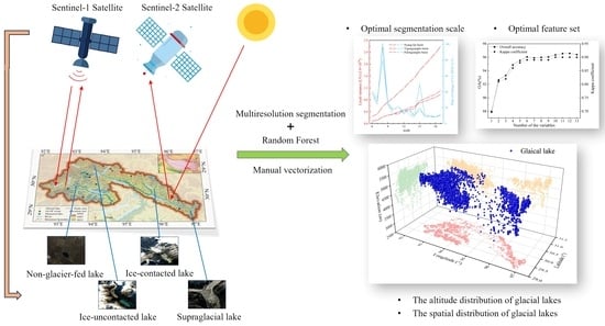
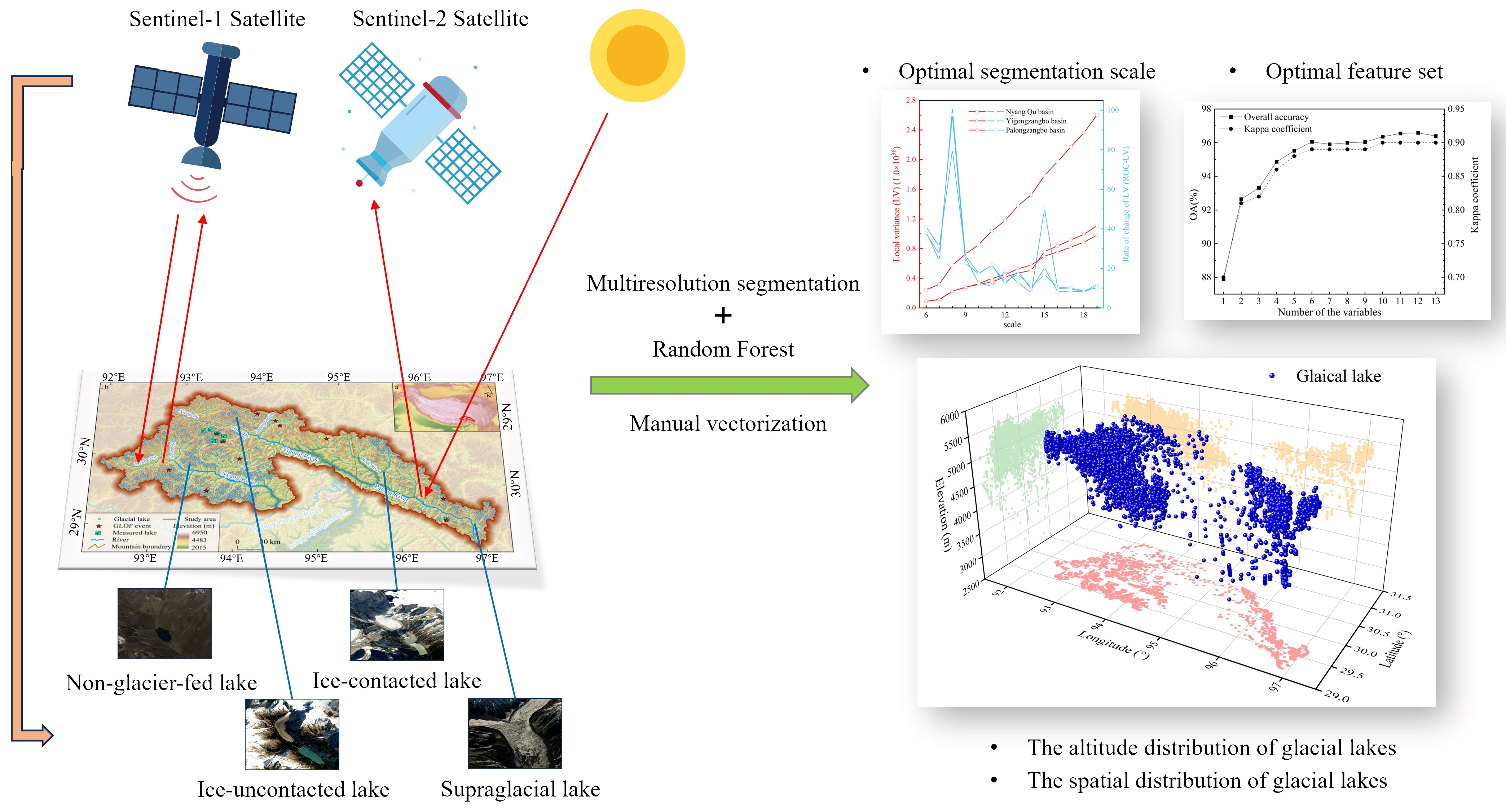
3. Data and Methods
3.1. Data
3.2. Methods
3.2.1. Polarization Mode Selection
3.2.2. Image Segmentation
3.2.3. Object Features’ Construction and Selection
3.2.4. Object Classification and Manual Vectorization
3.2.5. Error Assessment
3.2.6. Classification of Glacial Lakes
4. Results
4.1. Optimal Segmentation Scale
4.2. Optimal Feature Set
4.3. Distribution of Glacial Lakes
5. Discussion
5.1. Assessment of Glacial Lake Volume
5.2. Comparison with Other Glacial Lake Datasets

| Dataset Source | Latest Year | Minimum Area (km2) | Development Area | Count (Them) | Count (us) | Discrepancy |
|---|---|---|---|---|---|---|
| Shugar et al. [28] | 2015 | 0.05 | Within 1 km of glacier polygon in the RGI6.0 | 78 | 194 | 8 |
| Zhang et al. [17] | 2016 | 0.0027 | Within 10 km of glacier polygon in the RGI3.2 | 2072 | 2188 | 58 |
| Chen et al. [19] | 2017 | 0.0081 | Within 10 km of glacier polygon in the SCGI | 1081 | 1843 | 62 |
| Wang et al. [8] | 2018 | 0.0054 | Within 10 km of glacier polygon in the SCGI | 1565 | 2212 | 30 |
| Sequence Number | Name | Description |
|---|---|---|
| 1 | Incorrect extraction in other studies | Bare land (Figure 12a), glacial tongue (Figure 12c) or mountain shadow (Figure 12d) were misclassified as glacial lakes in other datasets. |
| 2 | Area threshold | Some glacial lakes in this study were excluded because they were smaller than the area threshold due to splitting (Figure 12b), being partially covered by ice floes (Figure 12e) or being interpreted from high-spatial-resolution images (Figure 12f). |
| 3 | Glacial lakes omitted in this study | Image quality resulted in some glacial lakes being missed in this study (Figure 12h). |
| 4 | Glacial lake specification | Other glacial lake inventories include rivers (Figure 12i) and lakes with dense vegetation growing around them (Figure 12g). |

5.3. Limitation and Prespective
6. Conclusions
Supplementary Materials
Author Contributions
Funding
Data Availability Statement
Acknowledgments
Conflicts of Interest
References
- Qin, D.; Yao, T.; Ding, Y.; Ren, J. Glossary of Cryospheric Science, 2nd ed.; China Meterological Press: Beijing, China, 2016; ISBN 978-7-5029-6473-3. [Google Scholar]
- Wang, X.; Liu, S.; Yao, X.; Guo, W.; Yu, P.; Xu, J. Glacier lake investigation and inventory in the Chinese Himalayas based on the remote sensing data. Acta Geogr. Sin. 2010, 65, 29–36. [Google Scholar]
- Yao, X.; Liu, S.; Han, L.; Sun, M.; Zhao, L. Definition and Classification System of Glacial Lake for Inventory and Hazards Study. J. Geogr. Sci. 2018, 28, 193–205. [Google Scholar] [CrossRef]
- Xu, D.; Liu, C.; Feng, Q. Dangerous glacial Lake and outburst features in Xizang Himalayas. Acta Geogr. Sin. 1989, 44, 343–351+385-352. [Google Scholar]
- López-Moreno, J.I.; Valero-Garcés, B.; Mark, B.; Condom, T.; Revuelto, J.; Azorín-Molina, C.; Bazo, J.; Frugone, M.; Vicente-Serrano, S.M.; Alejo-Cochachin, J. Hydrological and Depositional Processes Associated with Recent Glacier Recession in Yanamarey Catchment, Cordillera Blanca (Peru). Sci. Total Environ. 2017, 579, 272–282. [Google Scholar] [CrossRef]
- Yao, T. Tackling on Environmental Changes in Tibetan Plateau with Focus on Water, Ecosystem and Adaptation. Sci. Bull. 2019, 64, 417. [Google Scholar] [CrossRef]
- Song, C.; Sheng, Y.; Ke, L.; Nie, Y.; Wang, J. Glacial Lake Evolution in the Southeastern Tibetan Plateau and the Cause of Rapid Expansion of Proglacial Lakes Linked to Glacial-Hydrogeomorphic Processes. J. Hydrol. 2016, 540, 504–514. [Google Scholar] [CrossRef]
- Wang, X.; Guo, X.; Yang, C.; Liu, Q.; Wei, J.; Zhang, Y.; Liu, S.; Zhang, Y.; Jiang, Z.; Tang, Z. Glacial Lake Inventory of High-Mountain Asia in 1990 and 2018 Derived from Landsat Images. Earth Syst. Sci. Data 2020, 12, 2169–2182. [Google Scholar] [CrossRef]
- Yang, C.; Wang, X.; Wei, J.; Liu, Q.; Lu, A.; Zhang, Y.; Tang, G. Chinese glacial lake inventory based on 3S technology method. Acta Geogr. Sin. 2019, 74, 544–556. [Google Scholar]
- Slemmons, K.E.H.; Saros, J.E.; Simon, K. The Influence of Glacial Meltwater on Alpine Aquatic Ecosystems: A Review. Environ. Sci. Process. Impacts 2013, 15, 1794–1806. [Google Scholar] [CrossRef]
- Wang, X.; Ding, Y.; Zhang, Y. The Influence of Glacier Meltwater on the Hydrological Effect of Glacial Lakes in Mountain Cryosphere. J. Lake Sci. 2019, 31, 609–620. [Google Scholar] [CrossRef]
- Zhang, G.; Bolch, T.; Allen, S.; Linsbauer, A.; Chen, W.; Wang, W. Glacial Lake Evolution and Glacier–Lake Interactions in the Poiqu River Basin, Central Himalaya, 1964–2017. J. Glaciol. 2019, 65, 347–365. [Google Scholar] [CrossRef]
- Zheng, G.; Bao, A.; Allen, S.; Ballesteros-Cánovas, J.A.; Yuan, Y.; Jiapaer, G.; Stoffel, M. Numerous Unreported Glacial Lake Outburst Floods in the Third Pole Revealed by High-Resolution Satellite Data and Geomorphological Evidence. Sci. Bull. 2021, 66, 1270–1273. [Google Scholar] [CrossRef] [PubMed]
- Cook, K.L.; Andermann, C.; Gimbert, F.; Adhikari, B.R.; Hovius, N. Glacial Lake Outburst Floods as Drivers of Fluvial Erosion in the Himalaya. Science 2018, 362, 53–57. [Google Scholar] [CrossRef] [PubMed]
- Li, J.; Sheng, Y.; Luo, J. Automatic Extraction of Himalayan Glacial Lakes with Remote Sensing. J. Remote Sens. 2011, 15, 29–43. [Google Scholar]
- Wang, X.; Ding, Y.; Liu, S.; Jiang, L.; Wu, K.; Jiang, Z.; Guo, W. Changes of Glacial Lakes and Implications in Tian Shan, Central Asia, Based on Remote Sensing Data from 1990 to 2010. Environ. Res. Lett. 2013, 8, 044052. [Google Scholar] [CrossRef]
- Zhang, G.; Yao, T.; Xie, H.; Wang, W.; Yang, W. An Inventory of Glacial Lakes in the Third Pole Region and Their Changes in Response to Global Warming. Glob. Planet. Chang. 2015, 131, 148–157. [Google Scholar] [CrossRef]
- Wang, X.; Chai, K.; Liu, S.; Wei, J.; Jiang, Z.; Liu, Q. Changes of Glaciers and Glacial Lakes Implying Corridor-Barrier Effects and Climate Change in the Hengduan Shan, Southeastern Tibetan Plateau. J. Glaciol. 2017, 63, 535–542. [Google Scholar] [CrossRef]
- Chen, F.; Zhang, M.; Guo, H.; Allen, S.; Kargel, J.S.; Haritashya, U.K.; Watson, C.S. Annual 30 m Dataset for Glacial Lakes in High Mountain Asia from 2008 to 2017. Earth Syst. Sci. Data 2021, 13, 741–766. [Google Scholar] [CrossRef]
- Dou, X.; Fan, X.; Wang, X.; Yunus, A.P.; Xiong, J.; Tang, R.; Lovati, M.; Van Westen, C.; Xu, Q. Spatio-Temporal Evolution of Glacial Lakes in the Tibetan Plateau over the Past 30 Years. Remote Sens. 2023, 15, 416. [Google Scholar] [CrossRef]
- Wangchuk, S.; Bolch, T. Mapping of Glacial Lakes Using Sentinel-1 and Sentinel-2 Data and a Random Forest Classifier: Strengths and Challenges. Sci. Remote Sens. 2020, 2, 100008. [Google Scholar] [CrossRef]
- Wang, X.; Wu, K.; Jiang, L.; Liu, S.; Ding, Y.; Jiang, Z.; Guo, W. Wide expansion of glacial lakes in Tianshan Mountains during 1990–2010. Acta Geogr. Sin. 2013, 68, 983–993. [Google Scholar]
- Bhardwaj, A.; Singh, M.K.; Joshi, P.K.; Snehmani; Singh, S.; Sam, L.; Gupta, R.D.; Kumar, R. A Lake Detection Algorithm (LDA) Using Landsat 8 Data: A Comparative Approach in Glacial Environment. Int. J. Appl. Earth Obs. Geoinf. 2015, 38, 150–163. [Google Scholar] [CrossRef]
- Wang, J.; Chen, F.; Zhang, M.; Yu, B. ACFNet: A Feature Fusion Network for Glacial Lake Extraction Based on Optical and Synthetic Aperture Radar Images. Remote Sens. 2021, 13, 5091. [Google Scholar] [CrossRef]
- Zhang, M.; Chen, F.; Tian, B.; Liang, D.; Yang, A. High-Frequency Glacial Lake Mapping Using Time Series of Sentinel-1A/1B SAR Imagery: An Assessment for the Southeastern Tibetan Plateau. Int. J. Environ. Res. Public Health 2020, 17, 1072. [Google Scholar] [CrossRef] [PubMed]
- Zhang, B.; Liu, G.; Zhang, R.; Fu, Y.; Liu, Q.; Cai, J.; Wang, X.; Li, Z. Monitoring Dynamic Evolution of the Glacial Lakes by Using Time Series of Sentinel-1A SAR Images. Remote Sens. 2021, 13, 1313. [Google Scholar] [CrossRef]
- Zhang, M.; Chen, F.; Tian, B.; Liang, D. Using a Phase-Congruency-Based Detector for Glacial Lake Segmentation in High-Temporal Resolution Sentinel-1A/1B Data. IEEE J. Sel. Top. Appl. Earth Obs. Remote Sens. 2019, 12, 2771–2780. [Google Scholar] [CrossRef]
- Shugar, D.H.; Burr, A.; Haritashya, U.K.; Kargel, J.S.; Watson, C.S.; Kennedy, M.C.; Bevington, A.R.; Betts, R.A.; Harrison, S.; Strattman, K. Rapid Worldwide Growth of Glacial Lakes since 1990. Nat. Clim. Chang. 2020, 10, 939–945. [Google Scholar] [CrossRef]
- Liu, S.; Yao, X.; Guo, W.; Xu, J.; ShangGuan, D.; Wei, J.; Bao, W.; Wu, L. The contemporary glaciers in China based on the Second Chinese Glacier Inventory. Acta Geogr. Sin. 2015, 70, 3–16. [Google Scholar]
- Korzeniowska, K.; Korup, O. Object-Based Detection of Lakes Prone to Seasonal Ice Cover on the Tibetan Plateau. Remote Sens. 2017, 9, 339. [Google Scholar] [CrossRef]
- Nie, Y.; Liu, Q.; Liu, S. Glacial Lake Expansion in the Central Himalayas by Landsat Images, 1990–2010. PLoS ONE 2013, 8, e83973. [Google Scholar] [CrossRef]
- Zhao, H.; Chen, F.; Zhang, M. A Systematic Extraction Approach for Mapping Glacial Lakes in High Mountain Regions of Asia. IEEE J. Sel. Top. Appl. Earth Obs. Remote Sens. 2018, 11, 2788–2799. [Google Scholar] [CrossRef]
- Yang, Y.; Liu, Y.; Zhou, M.; Zhang, S.; Zhan, W.; Sun, C.; Duan, Y. Landsat 8 OLI Image Based Terrestrial Water Extraction from Heterogeneous Backgrounds Using a Reflectance Homogenization Approach. Remote Sens. Environ. 2015, 171, 14–32. [Google Scholar] [CrossRef]
- Ke, C.; Kou, C.; Ludwig, R.; Qin, X. Glacier Velocity Measurements in the Eastern Yigong Zangbo Basin, Tibet, China. J. Glaciol. 2013, 59, 1060–1068. [Google Scholar] [CrossRef]
- Qi, M.; Liu, S.; Yao, X.; Grünwald, R.; Gao, Y.; Duan, H.; Liu, J. Lake Inventory and Potentially Dangerous Glacial Lakes in the Nyang Qu Basin of China between 1970 and 2016. J. Mt. Sci. 2020, 17, 851–870. [Google Scholar] [CrossRef]
- Duan, H.; Yao, X.; Zhang, D.; Qi, M.; Liu, J. Glacial Lake Changes and Identification of Potentially Dangerous Glacial Lakes in the Yi’ong Zangbo River Basin. Water 2020, 12, 538. [Google Scholar] [CrossRef]
- Liu, J.; Yao, X.; Gao, Y.; Qi, M.; Duan, H.; Zhang, D. Glacial Lake Variation and Hazard Assessment of Glacial Lakes Outburst in the Parlung Zangbo River Basin. J. Lake Sci. 2019, 31, 1132–1143. [Google Scholar] [CrossRef]
- Niu, C.; Jiang, W.; Huang, X.; Xie, J. Analysis and Comparison between Two Object-Oriented Information Extraction Software of Feature Analyst and eCognition. Remote Sens. Inf. 2007, 2, 66–70+105. [Google Scholar]
- Drăguţ, L.; Csillik, O.; Eisank, C.; Tiede, D. Automated Parameterisation for Multi-Scale Image Segmentation on Multiple Layers. ISPRS J. Photogramm. Remote Sens. 2014, 88, 119–127. [Google Scholar] [CrossRef]
- Genuer, R.; Poggi, J.-M.; Tuleau-Malot, C. Variable Selection Using Random Forests. Pattern Recognit. Lett. 2010, 31, 2225–2236. [Google Scholar] [CrossRef]
- Zhang, L.; Gong, Z.; Wang, Q.; Jin, D.; Wang, X. Wetland Mapping of Yellow River Delta Wetlands Based on Multi-Feature Optimization of Sentinel-2 Images. Natl. Remote Sens. Bull. 2019, 23, 313–326. [Google Scholar] [CrossRef]
- Gardelle, J.; Arnaud, Y.; Berthier, E. Contrasted Evolution of Glacial Lakes along the Hindu Kush Himalaya Mountain Range between 1990 and 2009. Glob. Planet. Change 2011, 75, 47–55. [Google Scholar] [CrossRef]
- Hall, D.K.; Bayr, K.J.; Schöner, W.; Bindschadler, R.A.; Chien, J.Y.L. Consideration of the Errors Inherent in Mapping Historical Glacier Positions in Austria from the Ground and Space (1893–2001). Remote Sens. Environ. 2003, 86, 566–577. [Google Scholar] [CrossRef]
- Paul, F.; Huggel, C.; Kääb, A. Combining Satellite Multispectral Image Data and a Digital Elevation Model for Mapping Debris-Covered Glaciers. Remote Sens. Environ. 2004, 89, 510–518. [Google Scholar] [CrossRef]
- Fujita, K.; Sakai, A.; Nuimura, T.; Yamaguchi, S.; Sharma, R.R. Recent Changes in Imja Glacial Lake and Its Damming Moraine in the Nepal Himalaya Revealed by in Situ Surveys and Multi-Temporal ASTER Imagery. Environ. Res. Lett. 2009, 4, 045205. [Google Scholar] [CrossRef]
- Hanshaw, M.N.; Bookhagen, B. Glacial Areas, Lake Areas, and Snow Lines from 1975 to 2012: Status of the Cordillera Vilcanota, Including the Quelccaya Ice Cap, Northern Central Andes, Peru. Cryosphere 2014, 8, 359–376. [Google Scholar] [CrossRef]
- Yi, C.; Cui, Z. Classification and Sedimentary Types of Glacial Lakes in the Halasi River Catchment, the Altay Mountains, Xinjiang. Oceanol. Limnol. Sin. 1994, 25, 477–485. [Google Scholar]
- Mool, P.K.; Bajracharya, S.R.; Joshi, S.P. Inventory of Glaciers, Glacial Lakes and Glacial Lake Outburst Floods in Nepal; Hill Side Press (P) Ltd.: Kathmandu, Nepal, 2001; ISBN 978-92-9115-194-3. [Google Scholar]
- Duan, H.; Yao, X.; Zhang, Y.; Jin, H.; Wang, Q.; Du, Z.; Hu, J.; Wang, B.; Wang, Q. Lake Volume and Potential Hazards of Moraine-Dammed Glacial Lakes—A Case Study of Bienong Co, Southeastern Tibetan Plateau. Cryosphere 2023, 17, 591–616. [Google Scholar] [CrossRef]
- Zhang, G.; Bolch, T.; Yao, T.; Rounce, D.R.; Chen, W.; Veh, G.; King, O.; Allen, S.K.; Wang, M.; Wang, W. Underestimated Mass Loss from Lake-Terminating Glaciers in the Greater Himalaya. Nat. Geosci. 2023, 16, 333–338. [Google Scholar] [CrossRef]
- Cook, S.J.; Quincey, D.J. Estimating the Volume of Alpine Glacial Lakes. Earth Surf. Dynam. 2015, 3, 559–575. [Google Scholar] [CrossRef]
- Konovalov, V.G.; Rudakov, V.A. Remote Assessment of Reserve Capacity of Outburst Alpine Lakes. Lëd I Sneg 2016, 56, 235–245. [Google Scholar] [CrossRef]
- Lesi, M.; Nie, Y.; Shugar, D.H.; Wang, J.; Deng, Q.; Chen, H.; Fan, J. Landsat- and Sentinel-Derived Glacial Lake Dataset in the China–Pakistan Economic Corridor from 1990 to 2020. Earth Syst. Sci. Data 2022, 14, 5489–5512. [Google Scholar] [CrossRef]


| Trial Name | Fixed Variable | Iteration Range | Step |
|---|---|---|---|
| Shape weight determination | Scale parameter: 20 Compactness weight: 0.5 | 0.1–0.9 | 0.1 |
| Compactness weight determination | Scale parameter: 20 Shape weight: 0.2 (obtained from above trial) | 0.9–0.1 | 0.1 |
| Parameter | Value | Parameter | Value |
|---|---|---|---|
| Increment of scale parameter | 1 | Number of loops | 15 |
| Starting scale parameter | 5 | Shape weight | 0.2 |
| Use of hierarchy | 1 | Compactness weight | 0.8 |
| Rank of Variables | Name of Variables | Score |
|---|---|---|
| 1 | Mean combination of ascending-orbit and descending-orbit images for August 2022 | 2.68 |
| 2 | Slope | 1.29 |
| 3 | Mean combination of ascending-orbit and descending-orbit images for September 2022 | 1.06 |
| 4 | Mean combination of ascending-orbit and descending-orbit images for November 2022 | 0.94 |
| 5 | Ascending-orbit images for August 2022 | 0.93 |
| 6 | Descending-orbit images for November 2022 | 0.87 |
| 7 | Ascending-orbit images for September 2022 | 0.78 |
| 8 | Ascending-orbit images for November 2022 | 0.76 |
| 9 | Descending-orbit images for September 2022 | 0.75 |
| 10 | Mean combination of ascending-orbit and descending-orbit images for October 2022 | 0.74 |
| 11 | Ascending-orbit images for October 2022 | 0.73 |
| 12 | Descending-orbit images for August 2022 | 0.72 |
| 13 | Descending-orbit images for October 2022 | 0.45 |
| Area Scale (km2) | Volume Derived from This Study (106 m3) | Cook et al.’s [51] Volume (106 m3) | Konovalov et al.’s [52] Volume (106 m3) | ||
|---|---|---|---|---|---|
| Value | Error (%) | Value | Error (%) | ||
| <0.07 | 0.12 | 0.12 | 3.92 | 0.27 | 26.45 |
| 0.07–0.25 | 1.55 | 1.68 | 6.97 | 4.73 | 63.35 |
| 0.25–0.75 | 7.94 | 8.95 | 10.47 | 24.91 | 66.55 |
| 0.75–2.13 | 43.89 | 51.65 | 14.72 | 141.52 | 68.92 |
| >2.13 | 229.06 | 281.28 | 18.18 | 758.67 | 69.72 |
Disclaimer/Publisher’s Note: The statements, opinions and data contained in all publications are solely those of the individual author(s) and contributor(s) and not of MDPI and/or the editor(s). MDPI and/or the editor(s) disclaim responsibility for any injury to people or property resulting from any ideas, methods, instructions or products referred to in the content. |
© 2023 by the authors. Licensee MDPI, Basel, Switzerland. This article is an open access article distributed under the terms and conditions of the Creative Commons Attribution (CC BY) license (https://creativecommons.org/licenses/by/4.0/).
Share and Cite
Zhang, Y.; Zhao, J.; Yao, X.; Duan, H.; Yang, J.; Pang, W. Inventory of Glacial Lake in the Southeastern Qinghai-Tibet Plateau Derived from Sentinel-1 SAR Image and Sentinel-2 MSI Image. Remote Sens. 2023, 15, 5142. https://doi.org/10.3390/rs15215142
Zhang Y, Zhao J, Yao X, Duan H, Yang J, Pang W. Inventory of Glacial Lake in the Southeastern Qinghai-Tibet Plateau Derived from Sentinel-1 SAR Image and Sentinel-2 MSI Image. Remote Sensing. 2023; 15(21):5142. https://doi.org/10.3390/rs15215142
Chicago/Turabian StyleZhang, Yuan, Jun Zhao, Xiaojun Yao, Hongyu Duan, Jianxia Yang, and Wenlong Pang. 2023. "Inventory of Glacial Lake in the Southeastern Qinghai-Tibet Plateau Derived from Sentinel-1 SAR Image and Sentinel-2 MSI Image" Remote Sensing 15, no. 21: 5142. https://doi.org/10.3390/rs15215142