Article

Time Series of Land Cover Mappings Can Allow the Evaluation of Grassland Protection Actions Estimated by Sustainable Development Goal 15.1.2 Indicator: The Case of Murgia Alta Protected Area

National Research Council of Italy (CNR), Institute of Atmospheric Pollution Research (IIA), c/o Interateneo Physics Department, Via Amendola 173, 70126 Bari, Italy
*
Author to whom correspondence should be addressed.
Remote Sens. 2023, 15(2), 505; https://doi.org/10.3390/rs15020505
Submission received: 2 December 2022 / Revised: 5 January 2023 / Accepted: 13 January 2023 / Published: 14 January 2023

Abstract

:
Protected areas, or national parks, are established to preserve natural ecosystems; their effectiveness on the territory needs to be evaluated. We propose considering a time series of the SDG 15.1.2 indicator, “Proportion of important sites for terrestrial and freshwater biodiversity that are covered by protected areas, by ecosystem type”, to quantify the presence over time of grassland ecosystem in Murgia Alta (southern Italy), within the Natura 2000 and national park boundaries. Time series of remote sensing imagery, freely available, were considered for extracting, by Support Vector Machine classifiers, a time series of grassland cover mappings from 1990 to 2021. This latter was, then, used for computing a time series of the SDG 15.1.2 indicator. A high reduction (about 15,000 ha) of grassland presence from 1990 to 2004, the foundation years of the national park, followed by the increasing stability up to nowadays, was evaluated. Furthermore, grassland presence was evaluated in a 5-km buffer area, surrounding Natura 2000 boundary, revealing a continuous loss from 1990 up to now (about 500 ha) in the absence of protection actions. This study represents the first long-term analysis for the grassland ecosystem in Murgia Alta and the first effort to analyze a time series of the SDG 15.1.2 indicator. The findings can provide inputs to governments in monitoring the effectiveness of protection actions.

Graphical Abstract

1. Introduction

Natural and semi-natural grassland, hereafter collectively called grasslands, are one of the major ecosystems in the world, covering close to one-third of the Earth’s terrestrial surface [1,2] and 22% of the European terrestrial surface [3]. As such, they are essential contributors to global biodiversity [4]. Grasslands host unique biodiversity associated with high levels of fine-scale species diversity [5] and they are among the most species-rich habitats in agricultural landscapes [6]. According to the United Nations (UN) Convention on Biological Diversity [7], European Union (EU) member states have embraced the goal of preventing and safeguarding the reduction or loss of biodiversity with the legal tool of the Habitat Directive [8] and the Birds Directive [9] and the main policy strategy posed by the Natura 2000 (N2K) network including an ecological system of protected sites for long-term conservation of threatened natural ecosystems [10].
Yet, despite regulation in favour of grasslands, they are today one of the most endangered and threatened ecosystems in Europe [11] due to land use (LU) change, agricultural intensification, abandonment and urbanization [5]. In addition, the change of climate occurring to the globe can threaten grassland behaviour [12] and contribute to the loss of biodiversity (plants, insects, birds) and its related ecosystem services. Therefore, there is an urgent need to monitor grasslands over large extents to assess their current state in terms of the area covered [13]. This is the case of “Murgia Alta” N2K Protected Area (PA) in the Apulia region, southern Italy, characterized by grasslands ecosystems hosting numerous endemic habitats and rare species, hence, considered of crucial importance for the conservation of wildlife and priority species [14]. The monitoring of grassland areas is, therefore, crucial in order to evaluate the success of the protection measures on the territory due to the N2K network or the National Park Authority. This latter has been established since 2004. Evaluating the success of PAs in guaranteeing habitat preservation is the main objective in [8] reporting (art. 17), as well as of PAs in general [15].
Rough estimates of the extent of grasslands can be derived from free periodic mappings as those offered by the Copernicus land monitoring services, as Corine Land Cover (CLC) [16] or the pan-European High Resolution (HR) grasslands layer [17], but they often result inadequately. This may be due to the fact that they are not sufficiently accurate, mainly at a local scale, or released with a too wide time interval for supporting local decision-makers in providing an estimation of the protection actions in the territory [18].
A long-term study to investigate spatio-temporal dynamics of grasslands in Murgia Alta has never been carried out despite complaints of land degradation since the 1990s by local users such as farmers, shepherds and environmental experts.
Remote sensing (RS) can represent a useful support for monitoring in space and time wide areas for a long time and the current availability of high spatial resolution historical time series of satellite imagery, free of charge, offers the opportunity for the spatio-temporal investigations required.
Diverse classification approaches for grasslands mapping based on RS data have been implemented and deployed in the literature [19]. These algorithms usually include the automatic recognition from satellite data by using Artificial Intelligence (AI) techniques. Among the most recent literature, [20] has trained a Random Forest (RF) classifier for a multi-class problem, including grasslands, by using all the available Sentinel-2 images and reference samples from an existing database. Hence, they have worked at the country scale obtaining an F1-score less than 70% for natural grassland. Badreldin et al., (2021) [21] have trained an RF classifier for a multi-class problem, including grasslands, by using big RS data either from MODIS to generate a monthly average time series of the Normalized Difference Vegetation Index (NDVI) or from Sentinel-2 and Sentinel-1 missions to extract a further time series of spectral indices. They have paid particular attention to the selection of reference samples for training since ground-truthing is crucial in RS-based classification research; the more precise field data, the more accurate the classification will be, they declared. They have achieved 98.20% of user’s accuracy and 88.40% producer’s accuracy for native grassland. Abdollahi et al. (2022) [22] have considered a deep learning algorithm as the most recent Convolutional Neural Network (CNN) classifier for a 3-classes vegetation-based problem (i.e., grasslands, forest, other) by using as input a short time series of Sentinel-2 imagery and Enhanced Vegetation Index (EVI) obtaining an F1-score of 86% for grasslands. Adamo et al., (2020) [23] have explored the performance of an object-based knowledge-driven approach to classify very HR images for grasslands ecosystem mapping reporting 92.6%, 99.9% and 96.1% for grasslands user’s, producer’s accuracy and F1-score, respectively.
Fassnacht et al. (2015) [24] have focused on the consideration that vegetation cover and changes therein can be considered as indicators of degradation levels by analysing satellite images from different years. They were interested in degraded grasslands and considered locating the degraded areas by Landsat imagery. Li et al., (2020) [25] have also considered temporal changes in grasslands cover extracted by Sentinel-2 data, jointly with spatial heterogeneity indexes from MODIS imagery, for assessing degradation.
In this study, we aim to monitor grasslands cover in space and time in Murgia Alta to assess whether the ecosystem conservation has been threatened, thus, evaluating the effectiveness of protection actions on the territory. According to Tarantino et al., (2021) [18], intra-annual time series of four multi-seasonal Sentinel-2 data will be considered in order to take into account the phenological cycle of vegetation in the scene and reducing the computational effort respect to Inglada et al., 2017 [20]. We will adopt the supervised Support Vector Machine (SVM) classifier, for a multi-class problem, rather than deep learning algorithms that require relatively large training datasets to work well, and adequate infrastructure to be trained in a reasonable time [26]. With respect to RF, Grabska et al. (2020) [27] have argued that RF may struggle with less-common classes and corresponding imbalanced training data [28], while SVM may perform better in this case. Indeed, we are interested in grasslands layer so our training reference samples will be chosen more numerous for grasslands LC class and, mainly, selected at the local site scale to maximize the accuracy for the grasslands cover mapping.
Olsen et al., (2005) [29] considered examining the trend of landscape metrics over time as an alternative approach for ensemble investigations not only over a long period but also over intermediate periods; this approach could be important to informing management decisions on how particular interventions affect the sustainability of natural resources [30].
Sustainable Development Goals (SDGs) indicators are instrumental for the monitoring of countries’ progress towards sustainability goals as set out by the UN Agenda 2030. Earth Observation (EO) data can facilitate such monitoring and reporting processes, thanks to their intrinsic characteristics of spatial extensive coverage, high spatial, spectral, and temporal resolution, and low costs. EO data can, hence, be used to regularly assess specific SDG indicators over very large areas and to extract statistics at any given subnational level [31].
To address such concerns, in 2020, the Food and Agriculture Organization (FAO) introduced a new data collection approach that directly measures the indicators through a quantitative analysis of standardized land cover (LC) maps (European Space Agency Climate Change Initiative Land Cover maps—ESA CCI-LC) even though at a global scale (300 m spatial resolution).
Liu et al. (2019) [32] have added that the sustainable use of Earth resources and the specific research topics falling into SDG 15, devoted to the sustainable management of terrestrial ecosystems, involve satellite-based applications as LC/LU classification, change detection, vegetation monitoring, deforestation and biodiversity analysis.
Kavvada et al. (2020) [33] have analysed existing EO systems to generate data for SDG indicators. Cochran et al., (2020) [34] in a research paper, have demonstrated the uses of EO data to assist the multi-scale assessment of the SDGs. Liu et al., (2019) [32] have claimed that to achieve the goal of worldwide sustainable protection and utilization of terrestrial ecosystems, it is necessary to quantitatively assess the implementation of SDG 15 at all the administrative levels, especially at the grass-roots level. Hence, they have considered the whole framework, at the county scale, of SDG 15 composed of 14 indicators grouping them into three groups according to the application field: sustainable forest management (15.1.1, 15.2.1, 15.4.2 and 15.b.1), halt and reverse land degradation (15.3.1) and biodiversity conservation (15.1.2, 15.4.1, 15.5.1, 15.6.1, 15.7.1, 15.8.1, 15.9.1, 15.a.1 and 15.c.1).
Indicators SDG 15.1.2, 15.4.1 and 15.5.1 are limited to ‘PAs’, as their definition specifies so. Therefore, there is a clear need to use a map representing the PAs to extract such indicators. ‘PA’ variable is not an essential variable per se but can be considered as a socio-economic variable [35].
In our study, we will compute the time series of SDG 15.1.2 indicator “Proportion of important sites for terrestrial and freshwater biodiversity that are covered by PAs, by ecosystem type” by using time series of grasslands cover mappings extracted for Murgia Alta within N2K and National Park boundaries to estimate the effectiveness of protection actions for the safeguarding of grasslands ecosystem and its biodiversity.
Our findings could encourage protection actions by local authorities for preserving ecosystems such as grasslands along with their biodiversity.
The paper is organized as follows: Section 2 describes materials and methodology defining SDG 15.1.2 indicator and its computation. Section 3 reports findings and results about both time series of grasslands cover mappings and SDG 15.1.2 indicator trend computation. Section 4 discusses findings providing important information about the effectiveness of protection/conservation actions pursued over time in Murgia Alta and monitoring the progress of the Agenda 2030 for Sustainable Development.

2. Materials and Methods
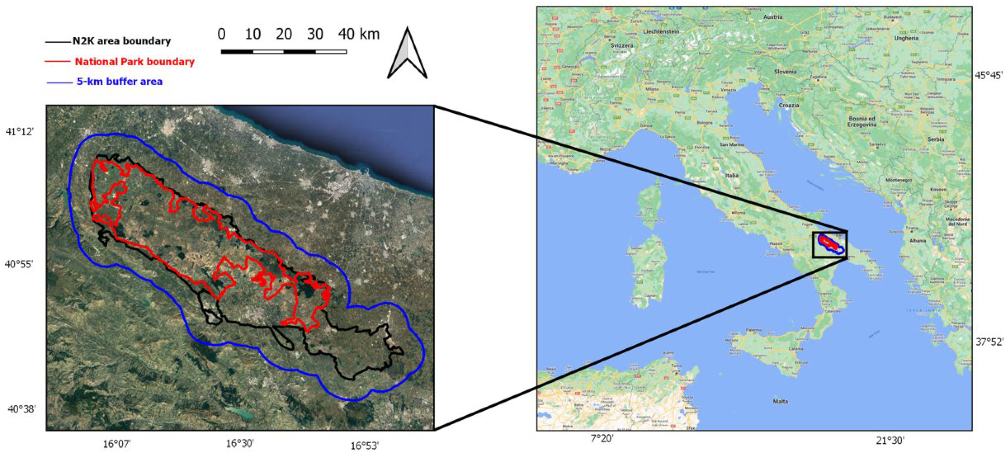
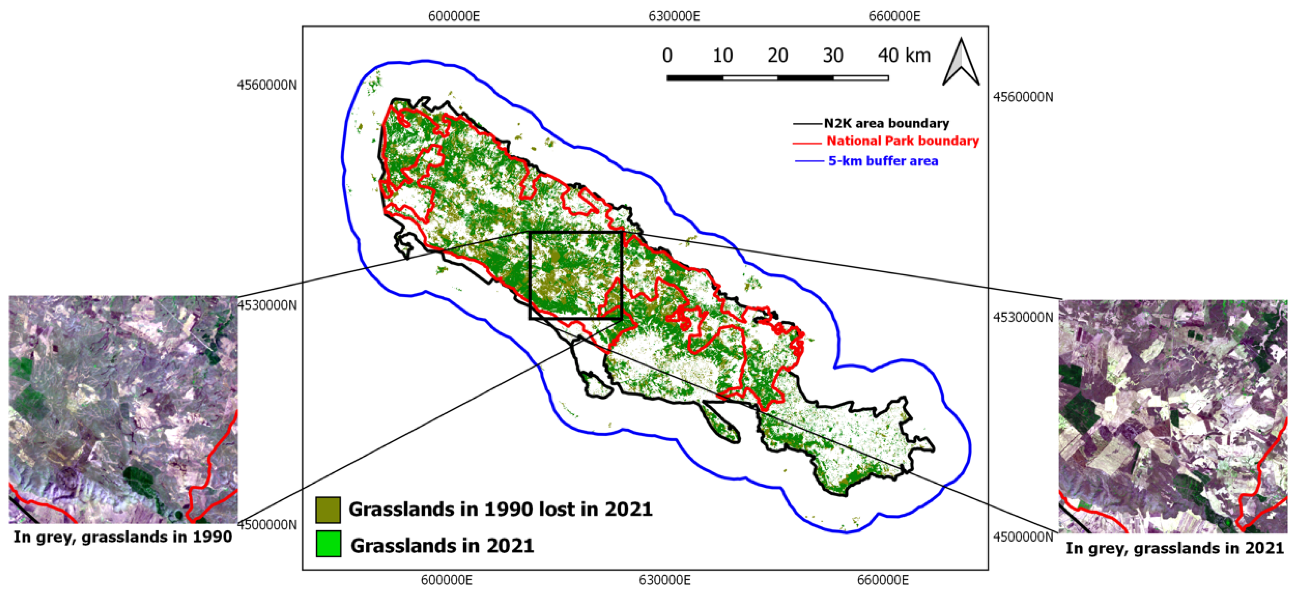
2.1. Study Site

The N2K Murgia Alta study site is a PA (IT9120007) located in the Mediterranean basin within the Apulia region, southern Italy. This is a Special Area of Conservation (SAC) [8] and in addition a Special Protection Area (SPA) [9], covering nearly 126,000 ha, with a national park (about 68,000 ha) included within since 2004. In addition, a 5-km buffer area surrounding the N2K boundary was considered (Figure 1) according to the Italian Institute for Environmental Protection and Research (ISPRA) suggestions for environmental impact assessment in the Natura 2000 PA [36].
The altitude of the area ranges from 285 to 680 m above the sea level and its climate is meso-Mediterranean, oceanic, and subcontinental with dry to sub-humid ombrotype [14]. The site is characterized by a typical Mediterranean agro-pastoral landscape with millennial LU history mainly occupied by semi-natural rocky dry grasslands (Figure 2), traditionally used as extensive pastures, while forest vegetation consists only of residual patches of downy oak (Quercus pubescens) woodlands and Aleppo pine (Pinus halepensis) plantations [37]. This area is considered of crucial importance for the conservation of wildlife [38]. In “Murgia Alta”, the semi-natural grassland ecosystem (with 62A0, 6210(*) and 6220* habitat types) hosts numerous regionally endemic and rare plant species but also many with trans-Adriatic distribution [14].
During the last 30–40 years, grasslands ecosystems have been exposed to tremendous impacts and accelerated processes of habitat degradation and fragmentation within and next to its borders. The pressures related to degradation range from:
  • The Common Agricultural Policy (CAP) which has driven the transformation of grassland pastures into cereal crops by stone clearance;
  • Fire events;
  • The illegal waste and toxic mud dumping on transformed areas which has caused heavy metal contamination of soils and aquifers;
  • The increasing of traditional legal and illegal mining activities and wind farm infrastructure;
  • The decrease of long-term average rainfall as a result of climate change and global warming;
  • Biotic contamination, i.e., woody encroachment [39] and the spreading of invasive species [40,41].
In 2004, the national park was instituted, therefore, leading to a series of protection and safeguard actions against biodiversity loss and ecosystem degradation.

2.2. Data Availability

A multi-temporal dataset consisting of four multi-season satellite imageries with less than 10% cloud cover was evaluated for each year considered, namely 1990, 2001, 2004, 2011, 2018 and 2021.. The choice of these years was based on the need for a long-term investigation and the absence of cloud cover along with the open satellite archive of ready-for-processing satellite imagery availability—time series imagery from Landsat satellite collection results from 1990 with well-assessed radiometric and geometric corrections. In addition, for comparison purposes, the selected years result close to (differing no more than ±2 years) the years of the two available products of CLC [16] (1990, 2000, 2006, 2012, 2018) and Copernicus Pan-European HR grasslands layer (2015, 2018) [17].
From 1990 to 2011, Landsat satellite imagery, at 30-m spatial resolution, was considered, whereas for 2018 and 2021 Sentinel-2 satellite data, 10-m spatial resolution was used. We chose to produce mappings with higher spatial details (10 m) for recent years in order to provide local management authorities to be able to rely on a useful and effective tool. Indeed, the latter are very interested in the recent situation to be managed. Nevertheless, the level of spatial detail of the Landsat images was considered sufficient to outline the general trend of the presence of grasslands over the long-term.
For each satellite image, the spectral bands in the visible (Vis)—near infra-red (NIR)—short wave infra-red (SWIR) were considered, resulting in 6 bands for Landsat 5 TM (except the thermic band) and 10 bands for Sentinel-2 A/B data.
Landsat data were freely downloaded from the United States Geological Survey (USGS) EarthExplorer portal [42] as Collection 2, Level 2, surface reflectance products, thus, atmospherically correct and orthorectified using ground data by USGS. The whole N2K PA, plus a 5-km buffer area surrounding the boundary, resulted in being covered by the track 188 and frames 31 and 32 floating, so a mosaicking step was realised after cropping the boundary of interest.
Sentinel-2 data were freely downloaded from the ESA Copernicus Open Access Hub [43] as L2A products which are surface reflectance and orthorectified imagery. Even in this case, the entire study area results were covered by the two tiles 33TXF and 33TWF, thus, their mosaicking was needed. The bands with native spatial resolution of 20 m (i.e., B5, B6, B7, B8A, B11, B12) were resampled, by applying the nearest neighbour algorithm at 10 m as those natives (B2, B3, B4, B8).
Table 1 shows the whole set of satellite imagery considered jointly with their acquisition dates.

2.3. Methodology

2.3.1. Time Series of Grasslands Cover

An inter-annual time series of six grassland mappings was obtained by working over a 30-year period from 1990 to 2021. Time series of grasslands cover maps will be used to examine their temporal trend.
The four images of each year, each one with its own bands, were stacked obtaining a multi-season raster dataset composed of 24 layers in the case of Landsat data, or of 40 hlayers for Sentinel-2 data. Each resulting multi-season dataset, for each year, was the input to a data-driven (supervised), pixel-based classification algorithm (machine learning) to obtain LC classified maps as output. A different classifier was trained for each year. Reference polygons for training each classifier and the subsequent validation of the output maps were considered. The polygons were collected through both in-field campaigns and a visual interpretation of available orthophotos for 2018. Such polygons were checked on the images related to the other years making use of aerial photos (where available) and the Google Earth historical database. For each year, the reference polygons were distributed in the whole scene according to the real percentage of presence of each class on the ground by a “stratified” sampling to ensure a minimum number of polygons—samples for each class (i.e., stratum) [44]. The reference pixels were divided into training and validation datasets randomly per each LC class. Approximately 70% and 30% of the samples for each class were considered for training and validation, respectively. Nearly 50% of the training and validation pixels were represented by grassland samples since this was the dominant LC in the scene and the class of greatest interest in this study, so high accuracy was required for this class. The cultivated herbaceous vegetation was represented by almost 25% of reference pixels since this was the second major class in the scene. The remaining area was covered by both natural needle-leaved evergreen and non-herbaceous cultivated classes. Table 2 lists the total number of training and validation pixels considered for grasslands. Columns 3 and 4 report, in brackets, the percentage of grasslands pixels with respect to the multi-class training and validation dataset, respectively.
Ground truth data are related to 12 LC classes, including grasslands, labelled according to the FAO-Land Cover Classification System (FAO-LCCS; Version 2) taxonomy [45] that is an open (expandable) classification system with a virtually infinite number of mutually exclusive classes. Furthermore, it offers a framework to integrate EO data with in- situ and ancillary data (e.g., lithology, soil aspects, soil surfaces), reducing uncertainties and class overlaps providing a higher level of detail [46,47,48,49]. Grasslands were coded as A12/A2.A6 “Natural Terrestrial Vegetation/Herbaceous.Graminoid”, according to FAO-LCCS2 taxonomy, thus, taking into account as it appears from remote sensing observations [23].
For the evaluation of multi-class LC mappings, an SVM classifier was trained for each year. SVM is a non-linear supervised classifier with no assumption on the data distribution and aimed at finding the optimal separating hyperplane that can divide the input dataset into the predefined number of classes [50,51]. It results particularly effective in high dimensional spaces [52] and is well-suited when small training data sets are available. Thus, SVM was adopted for our study. Following the recommendations reported in [53], in our study, a radial basis function was selected as kernel type while the penalty parameter chosen was taken as 100. According to [54], the gamma in the kernel function was chosen as the inverse of the band numbers used in the input data. SVM classifier was implemented by e1071 package in R 4.0. 3 open-source language in the RStudio IDE v1.3.1093 (www.rstudio.com) (accessed on 27 November 2022).
Then, from LC mappings produced as output, the grasslands layer was extracted. The whole workflow for obtaining the grasslands cover mapping, for each year considered, is shown in Figure 3.

Accuracy Assessment of Grasslands Cover Mappings

The protocol described in [55,56] and implemented in [57] was adopted for the classification accuracy assessment applied to obtain grasslands cover mappings. This protocol starts from the information obtained from the traditional Confusion Matrix (CM) [58] where the map categories (classes) (i = 1, 2, …, q) are represented by rows and the reference categories (j = 1, 2, …, q) by columns, both expressed as sample counts. Then, each cell of the CM is modified and reported in terms of the estimated area proportion pij, for the population in each cell i,j of the matrix, obtaining the population CM. More specifically, if i represents the mapped class and j the reference class, “population” is defined the full region of interest, and pij is, therefore, the value that would result if a census of the population was obtained (i.e., complete coverage reference classification). The specific formula for estimating pij depends on the sampling design used. For an equal probability sampling design (e.g., simple random and systematic sampling) and for stratified random sampling in which the strata correspond to the mapped classes, it can be obtained as:
pij = Wi nij/ni,
where Wi = Amapped,i/Atot is the proportion of the area mapped as class i, Amapped,i is the area mapped (hectares, ha) as class i in the map and Atot represents the total mapped area of the scene. For simple random and systematic sampling, Equation (1) represents an estimator recommended because it will have better precision than the estimators commonly used [58].
Substituting pij of Equation (1) into the formulas for overall accuracy (OA), user’s accuracy (UA) and producer’s accuracy (PA) according to [58] but rather considering the population CM, the modified estimators of OA, UA and PA with standard errors estimates can be obtained as [56]:
OA = J = 1 q p j j
U A i = p i i p i .
P A j = p j j p . j
In addition, the mean F1-score of the classification results was computed as a harmonic mean of precision and recall (5). Precision indicates how many pixels classified as true are actually true, while recall shows how many true pixels were correctly classified as true [59,60,61].
F 1 s c o r e = 2 × P r e c i s i o n × R e c a l l P r e c i s i o n + R e c a l l = 2 × U A × P A U A + P A
Lastly, the macro-averaged F1-score (or macro F1-score) [62] was computed as the arithmetic mean of all the per-class F1-score, hence, considering all classes equally important.

2.3.2. SDG 15.1.2 Indicator Computation

SDG 15.1.2 indicator “Proportion of important sites for terrestrial and freshwater biodiversity that are covered by PAs, by ecosystem type” belongs to the Target 15.1, “By 2020, ensure the conservation, restoration and sustainable use of terrestrial and inland freshwater ecosystems and their services, in particular forests, wetlands, mountains and drylands, in line with obligations under international agreements” within Goal 15, “Life on Land”. FAO is the custodian agency for this indicator and official metadata are available at SDG UN Metadata website [63].
The purpose of SDG 15.1.2 indicator is to provide a tangible measure of the effectiveness of actions adopted by the protection authorities for the conservation, restoration and sustainable use of ecosystems. The indicator is currently classified as Tier I. This means that the indicator is conceptually clear, has an internationally established methodology (i.e., standards are available) and data are produced regularly by countries [64]. The global indicator is compiled at the national level although, according to proposed metadata improvements, it could be disaggregated at the regional level and considering the variety of ecosystem types found in marine and terrestrial environments.
The basic computation methodology consists in a spatial overlap between polygons for PAs from the World Database on PAs (by the International Union for Conservation of Nature (IUCN) [65] or the Other Effective Area-based Conservation Measures (OECMs)) and those for terrestrial and freshwater Key Biodiversity Areas (KBAs) from the World Database of KBAs [66] (including Important Bird and Biodiversity Areas, Alliance for Zero Extinction sites [64]) insisting on the same area.
According to the World Database of KBAs, the KBA of interest for this study is site ID 2799 “Murge” (since 2002) (extension: 143,150 ha) [66].
According to the list of protection categories proposed by IUCN [65,66], Alta Murgia National Park and N2K site, both overlapping “Murge” KBA, belong to category II and IV, respectively. Category II explicitly refers to the national parks whereas category IV refers to the habitat/species management area. N2K site can be included in such latter category as the boundary area was designed as SPA and SAC from the Birds Directive and Habitats Directive, respectively, in 1998 (Figure 4).
In this study, SDG 15.1.2 was computed for each different IUCN protection categories. Grasslands ecosystem type was selected for computation and grasslands ecosystem mappings were used for the multi-temporal SDG 15.1.2. indicator estimation.
For N2K PA, SDG 15.1.2. indicator was computed as:
G r a s s l a n d s   c o v e r   w i t h i n   p o r t i o n   o f   N 2 K   P A   o v e r l a p p i n g   M u r g e   K B A   h a M u r g e   K B A   h a ×   100
Similarly, for the Murgia Alta National Park boundary:
G r a s s l a n d s   c o v e r   w i t h i n   portion   of   N a t i o n a l   P a r k   o v e r l a p p i n g   M u r g e   K B A   h a   M u r g e   K B A   h a ×   100
The unit of measurement at the numerator and denominator must be the same. In the Formulas (6) and (7) the hectare was adopted by convention.
Thus, the indicator estimates the percentage of coverage of the selected ecosystem within a PA, or in its portion contained in a reference KBA, with respect to this one.
To evaluate the impacts of the ecosystem protection and conservation policy adopted since the establishment of the PAs, the measurements of the indicator were repeated for different years in order to quantify the changes on the ecosystem coverage (loss/restoration) over time.
Thus, to facilitate the indicator calculation, a plugin in the Quantum Geographical Information System (QGIS) was developed and shared with the scientific community. Currently, the plugin is under evaluation by the QGIS user community. Once the evaluation process is completed, it will be available through the official QGIS plugin repository as SDG_15_1_2_calculator [67].
The plugin requires as input only the boundary maps of both KBA and PA considered and a cover map related to a generic ecosystem.

3. Results

The investigation, aiming to assess the long-term spatio-temporal dynamics of grasslands in Murgia Alta PA, was based on two main steps:
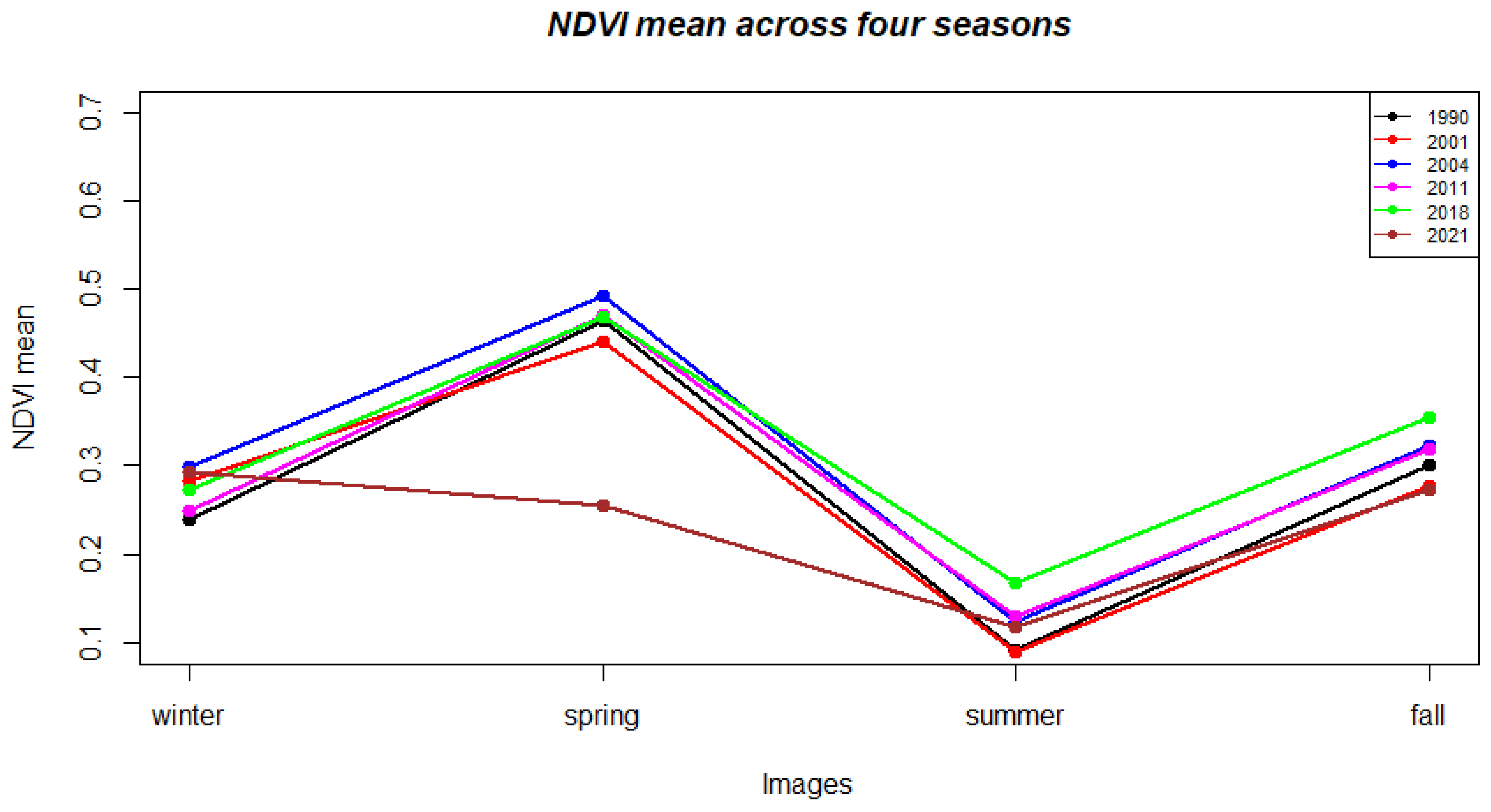
  • Generation of time series of LC maps and extraction of grasslands cover for the period 1990–2021 (one mapping for each of the following years: 1990, 2001, 2004, 2011, 2018, 2021);
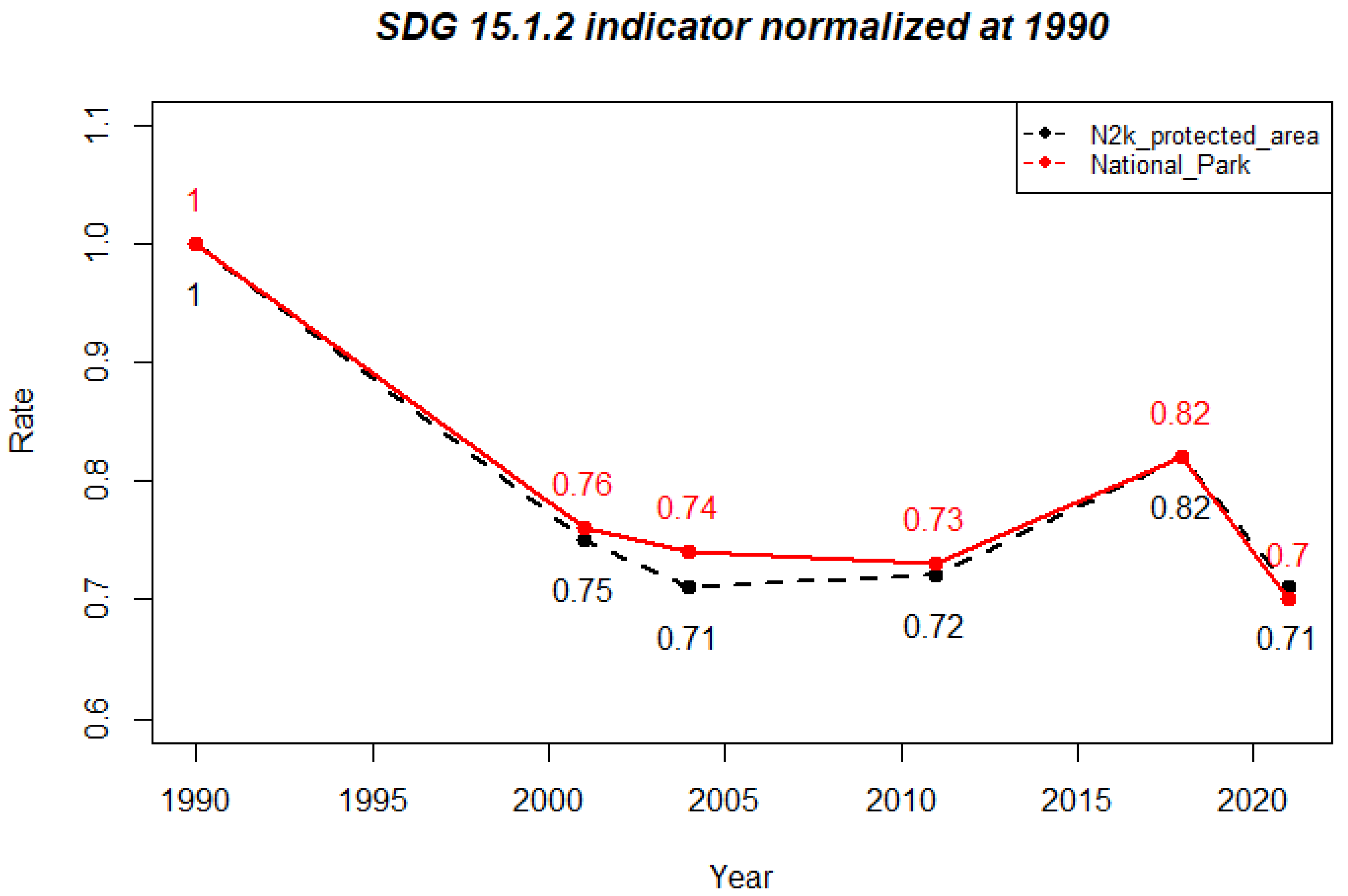
  • Computation of time series of SDG 15.1.2 indicator for the N2K PA and national park categories by using the time series of grasslands mappings and analysis of the temporal trend.
The findings obtained are presented separately below.

3.1. Time Series of Grasslands Cover

Figure 5 shows, for each year, the trend of NDVI mean value (computed in a window with grasslands presence in each year) for grasslands across the four selected seasonal images. The plot can allow to understand the specific behaviour in the phenological cycle of grasslands in the study site. According to the experts’ knowledge, grasslands achieve the highest biomass peak in spring, mainly April–May, and a second lowest peak in fall, mainly October–November. This expected trend can be found in the plot for the different years except for 2021 in which average temperatures above mean values in February and summer were registered [68]. This can explain the lowest value for the NDVI mean in spring considering that the selected image was acquired at the end of May (May 24th). Evidently, there was an early peak of biomass in 2021 and the selected image does not contain this information to be used for classification. This can explain the lowest OA obtained for the 2021 grasslands mapping.
As an example, Figure 6 shows the multi-class LC mapping produced for 2021 and the list of LC classes with description and code according to FAO-LCCS2 taxonomy.
Table 3 shows the list of OAs (%) and macro F1-scores (%) of the classified multi-class time series of LC mappings obtained by the supervised pixel-based classification approach described in sub-Section 2.3.1 for the whole 5-km buffer area surrounding the N2K boundary. The OA values resulted greater than 90% and macro F1-score not lower than 82%, hence, confirming the high level of reliability of the mappings produced.
In Figure 7, Figure 8 and Figure 9, grasslands cover layers extracted from the classification processing are shown, for each year, on the right column, whereas the available CLC mappings [16] considered for comparison purposes are reported on the left.
Figure 7 reports the classified mappings obtained for 1990 and 2001 compared with CLC mappings for 1990 and 2000, respectively. For our study, 1990-year mapping represents the starting point further back in time and 1990–2001 is the longest period (11 years) investigated between one mapping and the next.
Before the year 2000, CLC mappings were being updated without a regular frequency, as happened later, so after the first mapping of 1990 the next updating occurred after 10 years. As is well known, CLC is based on a different taxonomy (than the one used in our map, i.e., FAO-LCCS2). Thus, both 231 “Pastures” and 321 “Natural Grasslands” classes in CLC mappings were selected as representing the grasslands layer to be considered in this study.
Figure 8 shows the resulting mappings for 2004 which can be considered as the reference status for the grasslands presence for assessing the effectiveness of the institution of the national park which occurred in that year. The National Park Authority launched a series of safeguard actions for the protection of the grasslands ecosystem.
The mappings obtained for 2004 and 2011 vs. CLC mappings for 2006 and 2012, respectively, are reported in Figure 8. Starting from 2000, CLC mappings were updated every 6 years, according to the request of [8].
Figure 9 shows the mappings obtained for 2018 and 2021 vs. CLC and Copernicus HR grasslands layer mappings, both for 2018. Nowadays, no ancillary products are available to be compared with the classified map obtained for 2021.
Thanks to the availability of Sentinel-2 data, mappings at 10 m spatial resolution were achieved since 2018. Hence, for the same year, the Copernicus HR grasslands layer at 10-m spatial resolution was, also, considered.
Table 4 reports information about the accuracy of the obtained time series of binary grasslands/non-grasslands cover, where grasslands layer was extracted from multi-class classification, for the whole N2K boundary plus the 5-km buffer area surrounding. For quantitative comparison purposes, CLC and Copernicus grassland layers were validated by considering the same validation dataset used for validation of the classified mappings which differ no more than ±2 years. The results are also reported in Table 4.

3.2. Grasslands Cover Temporal Trend

Results of the computation of SDG 15.1.2 indicator for each year are shown in Table 5 for the time series of LC obtained by supervised classification and for CLC and Copernicus HR grasslands products considered for comparison purposes. SDG 15.1.2 indicators were computed within the N2K PA boundary (Category IV [65,66]) and the national park boundary (Category II [65,66]) by the grasslands ecosystem. In addition, grasslands cover within the 5-km buffer area surrounding the N2k boundary is reported.
Table 5 shows in chronological order the different grasslands mappings available from the different sources such as supervised classification, CLC or Copernicus in order to appreciate the agreement between the different products which differ each other no more than ±2 years to be compared. A further Copernicus HR grasslands layer available for 2015 [17] was not considered, since the time gap from other products (immediately previous or following) would have been 3 years. The last CLC product results for 2018: for this year products from three different sources are available.
For 1990, a significant difference (about 10%) has emerged in the values of SDG 15.1.2 indicator between the classified mapping and CLC layer (34.21% and 24.71%, respectively) in the N2K PA, and it has resulted slightly lower (about 5%) in the national park area (23.44% and 17.99%, respectively). About ten years later, comparing classified mapping for 2001 with CLC for 2000, such a difference, substantially, has disappeared as the values of the SDG 15.1.2 indicator result somewhat compatible (25.49% vs. 24.00%, respectively, for N2K PA and 17.92% vs. 17.66%, respectively, for the national park area). This can be explained as a clear inaccuracy (underestimation) in the older CLC product that was later improved. In any case, for CLC products, SDG 15.1.2 indicator values always have resulted lower than those from classified mappings. In 2018, the underestimation of CLC product with respect not only to the classified mapping (about 5%) but also to Copernicus layer (about 6%) has been evident. Indeed, the latter has resulted quite compatible with the SDG 15.1.2 indicator value obtained from the classified mapping (29.52% vs. 28.12%, respectively, in the N2K PA and 19.09% vs. 19.16%, respectively, in the national park area).
The resulting temporal trends can be better estimated by plotting the quantitative results of Table 5 as in Figure 10 which shows, on the same plot, the temporal trend, during the period 1990–2021 of SDG 15.1.2 indicator for grasslands ecosystem from the time series of classified mappings. The plotted values have been computed within the N2K PA and the national park boundaries and normalized to the 1990 data for assessing possible differences between the two trends beyond the absolute values of each one.
Both the plots show the same temporal trend—a significant reduction of grasslands can be assessed from 1990 to 2001. The reduction continued more slowly until 2004, when the national park authority was established, and then, substantially, the trend results having stabilized in the following years until 2021.
Below, Table 6 reports the change matrix related to the transitions of grasslands between 1990 and 2001, which is the period characterised by the highest grasslands reduction; the main transition results are cultivated areas (about 34%), mainly herbaceous, with about 1.5% to burn areas.
In 2018, a slight increase can be evaluated, probably due to the regrowth of grasslands on those areas affected by fires previously, followed by a successive decrease registered for 2021. Below, Figure 11, Figure 12 and Figure 13 can explain this trend.
In the long-term period, new areas of grasslands can be detected in the period 1990–2018, particularly due to natural colonization of burned forest surfaces (Figure 11).
In the short-term period:
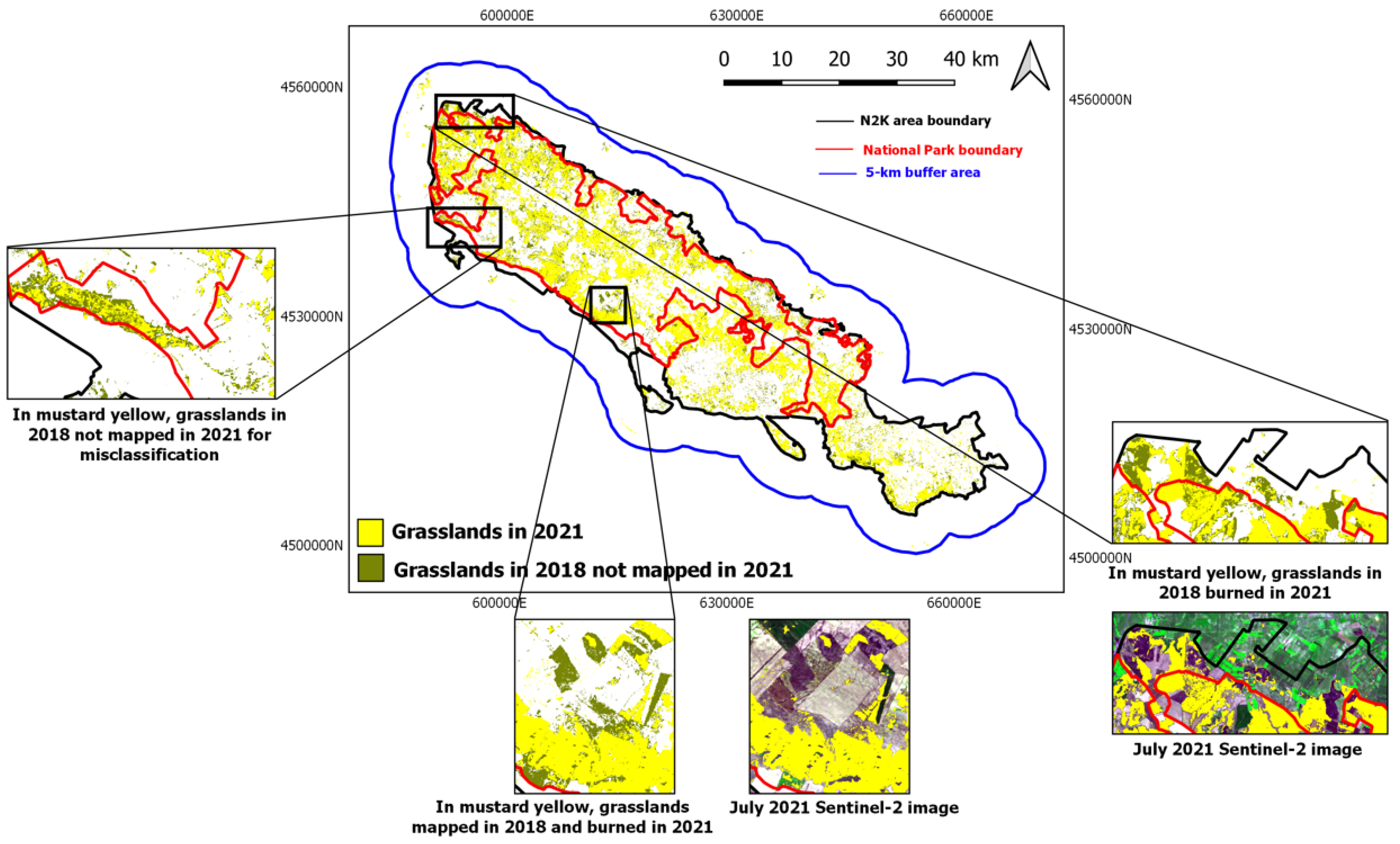
  • Comparing 2011 and 2018: important large fire events (mapped from the official fire registry) which happened after 2011 in forested areas can be focused on. One fire event happened in 2012 and the other two events happened in the same area in July 2011 (where partial regrowth of grasslands was already detected with the 2011 mapping by using August and October images for the mapping) and in 2015 for the second time (Figure 12). Hence, these fire events can allow to explain the 2018 grasslands increase with respect to the previous one in 2011.
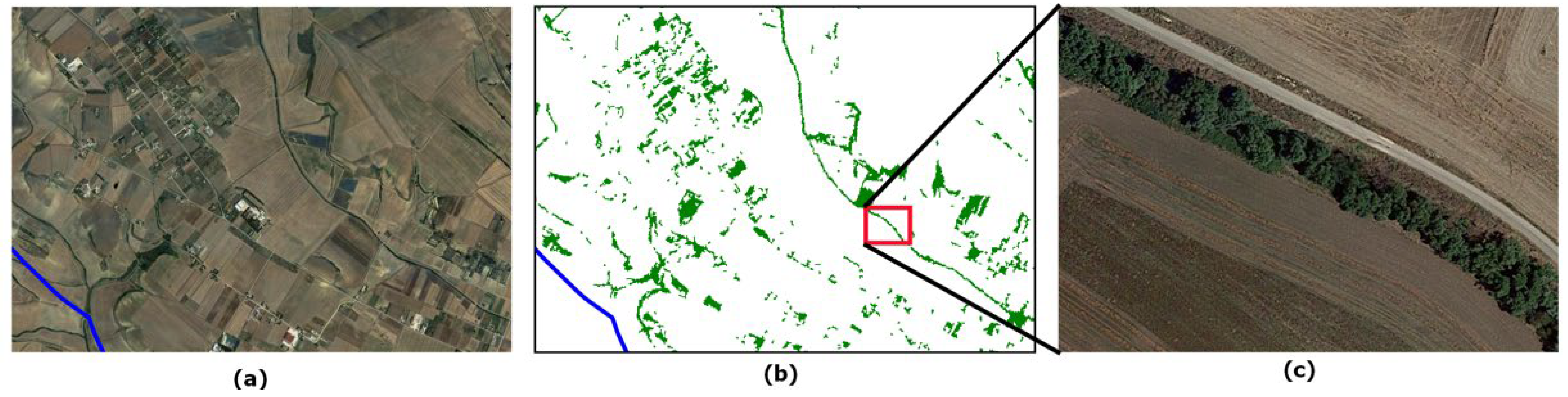
  • Comparing 2021 and 2018: either several areas with misclassification (2021 grasslands mapping reported the lowest OA) can be evidenced or recent burn areas for which no official mapped data are available from the official fire registry. Some of these areas are located outside the national park boundary (Figure 13). Hence, these considerations can allow to explain the 2021 grasslands lost with respect to the previous 2018 mapping.
Since KBA does not cover the 5-km buffer area surrounding the N2K boundary, the estimation of the SDG 15.1.2. indicator in this area was not possible, hence, in Table 5, in last column, grasslands coverage has been reported. Although there was a small presence of grasslands in the area, a continuous decreasing temporal trend of grasslands can be observed over the 30-year period analysed, with an overall loss of about 500 ha.

4. Discussion

This study aims to assess the long-term spatio-temporal evolution of grasslands ecosystem presence in Murgia Alta N2K PA, southern Italy. Several grassland habitats are endemic in this area and their conservation is considered of crucial importance by local authorities and decision makers responsible for environmental management. Hence, the need for periodic monitoring of protection actions implemented along with the search for a related indicator to assess their effectiveness on the territory and which can result as suitable, internationally recognized and easy to calculate, emerges. Within this framework, the use of time series of satellite imagery in the optical spectrum along with in-field data and AI techniques have been considered to monitor such grasslands ecosystems.

4.1. Time Series of Grasslands Cover Mappings

The free-of-charge availability of time series of HR satellite imagery, mainly from Landsat and Sentinel-2 missions, has offered the possibility for a long-term (three decades from 1990 to 2021) study on a wide area as Murgia Alta N2K PA (126,000 ha) that has never been investigated for such a long period. Grasslands are the dominant ecosystem in this area with large patches detectable with 10–30 m spatial resolution (by considering Sentinel-2 or Landsat imagery, respectively). Local experts’ measurements have been collected only recently, and there is a lack of information back in the past enlarged to the entire PA, at the local scale.
Four multi-seasonal satellite images for each year were considered to produce six LC mappings in the period 1990–2021 (for 1990, 2001, 2004, 2011, 2018, 2021) investigated by using a supervised, pixel-based, classification approach through SVM classifiers. The supervised approach was possible because of the availability of ground-truth data for 2018 collected during in-field campaigns and visual interpretation of available orthophotos for training classifiers (one for each year). The availability of reference data for the other years, mainly back in time, represents a real open challenge. De Simone et al. (2021) [31], working at the global scale, had the opportunity to consider databases already available for multiple years to be used for reference data selection. Working at the local scale, we needed to check the available reference data over each year under investigation through an accurate photointerpretation of available aerial photos and Google Earth historical database to assess whether any changes had occurred. Hence, at the local scale, only a semi-automatic approach can be followed. Special attention was paid for grasslands samples representing the target LC class of this study. Therefore, the percentage of grasslands samples represented more than 50% of the whole multi-class dataset for each yearly mapping (Table 2).
As a result, a multi-temporal/multi-class ground truth dataset was obtained. According to [18], a multi-class was preferred to a binary (grasslands/non-grasslands) classification since higher accuracy and lower misclassifications were obtained by the multi-class classifier. The multi-class LC mappings produced have great accuracy resulting in an OA value not lower than 90% (the lowest value equal to 90.73 ± 0.37% for 2021) and macro F1-score not lower than 82% (Table 3) among the different mappings. Similarly, the OA values obtained for the binary grasslands/non-grasslands classified mappings (Table 4) resulted not lower than 95.70 ± 0.07% (for 2021). In the different mappings, quite high UA and PA values (up to 98.93 ± 0.04% and not lower than 77.81 ± 0.07%, respectively) with the lowest F1-score equal to 86.61% (for 2021) resulted for grasslands. The lowest results for 2021 mapping, although being the most recent, can be explained for the average temperatures above mean values in February and summer which caused probably an early peak of biomass usually happening in April–May, so that the selected image of the end of May 2021 lost this information (Figure 5).
The highest F1-score value equal to 98.33% resulted from the classified mapping of 2018.
According to [18], as an alternative to the extraction of classified mappings, other available products as CLC grasslands layer or the HR grasslands Copernicus service were considered and compared, but on the largest whole N2K PA. These freely-available products results are not so accurate and reliable since (i) they are not annually updated. Indeed, CLC inventory was initiated in 1985 even though the first product was released labelled as 1990: hence, a sort of temporal mismatch exists. Further product updates have been produced in 2000, 2006, 2012, and 2018. According to the CLC products timeline, for comparison purposes, the classified mappings were extracted for the same year, 1990, as the further back in time starting point followed by the next mapping after 11 years (2001) which represents the longest period analysed; then the investigation pursued more regularly in time. Furthermore, Copernicus HR grasslands layers are not regularly updated and provided for 2015 and 2018 only, thus, (ii) both services are produced at a pan-European scale even though each one was at a different spatial resolution (100 m and 10 m for CLC and Copernicus products, respectively); (iii) CLC is a multi-class product with a different taxonomy—both 231 “Pastures” and 321 “Natural Grasslands” classes were considered to represent grasslands layers as expressed by FAO-LCCS2 taxonomy considered in our classified mappings; and (iii) Copernicus product results are noisy and affected by misclassification (with overestimation particularly emphasised in the 5-km buffer area where 15,823 ha of grasslands with many scattered pixels are mapped whereas CLC product has no grasslands presence in this area due to its underestimation and coarse spatial resolution), as shown in Figure 14 where grasslands presence results are mapped all along the road (Figure 14b), whereas dense tree canopies can be recognized from aerial photos (Figure 14c).
To evaluate the reliability of CLC and Copernicus HR grasslands layers compared to the time series of classified mappings produced, this work has considered satellite imagery acquired no more nor less than 2 years with respect to the years of the available products. The presence of cloudiness represented a limitation for optical satellite acquisitions, and it has been considered for the choice of multi-seasonal imagery, hence, those years characterized by a dominant clear sky were preferred.
The OA values for CLC layers resulted not higher than 90.59 ± 0.96% (for 2000) and F1-score values range between 64.01% (for 2018) and 73.03% (for 2000), respectively. In addition, for a qualitative analysis, from Figure 7, Figure 8 and Figure 9 the low accuracy and the low level of detail due to the coarse spatial resolution of the CLC products can be appreciated.
Compared to the higher OA of the classified product for 2018 (99.45 ± 0.02%), Copernicus grasslands mapping results in a lower OA equal to 88.75 ± 0.10% even though greater than the one of the CLC product (86.08 ± 1.03%). The same for the F1-score values resulting equal to 79.35% vs. 98.33% for the Copernicus and classified product, respectively.
Nowadays no ancillary products are available to be compared with the classified map obtained for 2021.
Hence, the freely-available mappings produced at the European scale (detail level) that can be considered for the assessment of spatio-temporal trends in grasslands are not a reliable product at the local scale, as required in this study, due to both temporal and spatial constraints characterizing them. Thus, in this paper, grasslands mappings were obtained at the local scale by training, with local reference samples, supervised machine learning classifiers which were fed in input with four multi-seasonal satellite images. Furthermore, grasslands, which was the LC class of greatest interest in the study, were represented by nearly 50% pixels of the whole multi-class reference dataset.
The findings obtained suggest that the mapping accuracy for the LC of interest can be improved by specializing ground truth reference data for the class of interest more than for the other classes, hence, reducing the efforts in the search for a reliable training data set.

4.2. Grasslands Cover Spatio-Temporal Trend

Time series of grasslands mappings obtained as described above were considered to assess the spatio-temporal trend of grasslands presence in Murgia Alta study site. This represents the first attempt of a long-term analysis at the local scale for such a large endemic ecosystem subject to conservation actions by the N2K network and the National Park authority whose effectiveness on the territory should be monitored. Therefore, in order to address the need to use a measure that was internationally recognized, achieving SDGs and providing the estimation of grasslands ecosystem conservation on a specific territory, this study has considered the SDG 15.1.2 indicator by the UN. Furthermore, this indicator can allow for estimating whether the areas are adequately under protection for the long-term conservation of natural habitats and ecosystems.
The suitability of the SDG 15.1.2 indicator, assigned the ecosystem, to be declined at varying categories of protection on the territory, has represented a good fit for our study to express an estimate for the conservation of biodiversity within the boundaries of the N2K network and the national park, both within the territory of Murgia Alta site. The computation of a percentage related to the extent of the reference KBA insisting on the specific territory can allow the introduction of a sort of normalized estimation.
Unlike other indicators in the group of SDG 15 already being considered in different studies as in [31], SDG 15.1.2 indicator needs to be more widely employed and disseminated to appreciate if it can result as suitable as a reference indicator, according to what has been applied in this study. Liu et al., (2019) [32], considering the connotation of different levels of biodiversity (genetic diversity, species diversity, ecosystem diversity and landscape diversity) in China, selected five sub-indicators that were most closely related to the biodiversity at each level and constructed a biodiversity index based on RS data to identify important areas for biodiversity. Hence, they referred the computation of SDG 15.1.2 to the BI computation. However, to the best of our knowledge, in the current literature, no studies have implemented the time series of SDG 15.1.2 indicator at local level and our study may represent the first effort to compute the time series of SDG 15.1.2 indicator as well as we propose. In our opinion, the latter can allow to estimate the evolution trend in time and space and to detect changes of a specific ecosystem giving indications about the effectiveness of the different protection measures on the territory for a long-term analysis as the 30-years period 1990–2021 for the grasslands ecosystem in Murgia Alta within the N2K PA and national park boundaries.
A significant indication of the actual effectiveness of protection actions can be derived considering what has occurred immediately outside the area under protection. For this area the computation of SDG indicator 15.1.2 was not possible due to this area not being covered by any KBAs. Furthermore, indications about future actions, that local decision makers might take, can be possible from this kind of analysis.
The findings, expressed as SDG 15.1.2 indicator percentage values, resulting within N2K boundary show a significative reduction (about 10 percentage points) of the presence of the ecosystem from 1990 (34.21%) to 2004 (24.28%) corresponding to about 15,000 ha, more emphasised (about nine percentage points) up to 2001 (25.49%) of about 13,000 ha, as shown by Figure 10, then followed by a substantial stabilization. The same trend can be confirmed within the national park boundary with a reduction of about 9000 ha (about six percentage points) from 1990 (23.44%) to 2004 (17.24%), more emphasised (5.5 percentage points) up to 2001 (17.92%) of about 8000 ha. The lower values in the national park can be explained since this area is a subset of the N2K PA. Considering that the national park was instituted in 2004, those outcomes offer the possibility for a two-fold consideration:
  • National park action on the territory has resulted effective to preserve the grasslands ecosystem conservation;
  • National park protection actions have resulted more effective than those of N2K network implemented in the area since 1998.
The long-term monitoring of 1990–2021 in space and time can be evaluated through Figure 15 where 2021 grasslands mapping was overlapped with that for 1990, providing evidence (in mustard yellow colour) about temporal and spatial grasslands lost.
The important contribution from a time series of LC mappings is represented by the possibility not only to detect LC changes but also to know the from-to LC classes [57] involved in the change during time. In our case study, most of the changes have been found towards cultivated areas (as an example Figure 16) or burned areas (Table 6).
Outside PA, in the 5-km buffer area surrounding, the trend of the presence of grasslands can be evaluated in terms of presence in hectares due to no KBAs covering the study area. Here the presence of grasslands, although not so extensive to be mapped by the coarse spatial resolution of the CLC product, has suffered a continuous declining trend starting from 1990 to the present (Table 5, last column) with an overall loss of about 500 ha. These findings can allow to evaluate the effects of the absence of any protection and safeguard actions in the buffer area differently from what has happened within the N2K and national park boundaries.
According to the confidence from the outcomes of the study it can be argued that the presence of preservation and conservation actions on the territory as those carried out by the establishment of a PA or, even more effective, of the national park authority have been essential to protect the grasslands ecosystem from its continuous degradation.

5. Conclusions

The aim of the present study was to assess the spatio-temporal dynamic, in the long-term, of the presence of grasslands which hosts endemic habitats and is the dominant ecosystem in “Murgia Alta”, a N2K network PA with a national park within, exposed to degradation. The free availability of time series of RS data was exploited to obtain, by machine learning supervised algorithms (SVM) trained at local scale, time series of LC mappings for grasslands cover. Those mappings were considered for the evaluation of spatio-temporal trends for the presence of grasslands in the study area by estimating the time series of the SDG 15.1.2 indicator. The latter was computed for different conservation categories: the N2K PA and the national park categories.
From the findings the following has emerged for assessing the monitoring of grasslands presence:
  • RS is a powerful tool for environmental monitoring because it provides both temporal and spatial information [11];
  • The availability of free time series of satellite data at high spatial resolution can offer the possibility for a long-term analysis on wide areas at a local scale. As a result, the costs for expensive in-field campaigns can be reduced and updated time series of LC mappings can be available whenever needed;
  • Working at the local scale along with using AI techniques allow to obtain more accurate mappings than those offered by the available Copernicus services;
  • Time series of SDG 15.1.2 indicator can allow the estimation of the spatio-temporal dynamics of an ecosystem in relation to the levels of protection featured on the territory, providing support in estimating the effectiveness and impact of protection and conservation actions.
Grasslands ecosystem in Murgia Alta N2K PA has been reduced from about 50,000 ha to 35,000 ha over the 30-year period of 1990–2021—with the establishment of the National Park Authority, the ecosystem degradation process has somewhat stopped.
From the evaluation of what has been detected inside and outside the protection boundaries, several directives to local or EU decision makers can be provided to direct policies toward the introduction of new PAs and/or the implementation of ecological networks between existing PAs [69] as possible initiatives for preserving biodiversity and the proper functioning of ecosystems.

Author Contributions

Conceptualization, C.T.; methodology, C.T. and M.A. (Mariella Aquilino); software, C.T. and M.A. (Mariella Aquilino); validation, C.T., M.A. (Mariella Aquilino), M.A. (Maria Adamo) and R.L.; formal analysis, C.T.; investigation, C.T. and R.L.; resources, C.T., M.A. (Mariella Aquilino) and R.L.; data curation, C.T.; writing—original draft preparation, C.T., M.A. (Mariella Aquilino) and R.L.; writing—review and editing, C.T. and M.A. (Maria Adamo); visualization, C.T.; supervision, M.A. (Maria Adamo); project administration, C.T.; funding acquisition, C.T. All authors have read and agreed to the published version of the manuscript.

Funding

This research was funded by the LIFE Preparatory Project “Remote sensing-oriented nature-based solutions towards a NEW LIFE FOR DRYLANDS”, Grant Agreement: LIFE20PRE/IT/000007 and POR Puglia 2014/2020—Azione 6.5—Azioni di monitoraggio di Rete Natura 2000 su habitat e specie della Puglia (D.G.R. 150/2020 e d.d. n. 108 del 06.08.2020) “Monitoraggio di Habitat e Specie nel sito Murgia Alta”.

Data Availability Statement

Not available.

Acknowledgments

The authors are grateful to “Murgia Alta” National Park Authority for the remarkable ecological support and to Palma Blonda for the valuable suggestions.

Conflicts of Interest

The authors declare no conflict of interest.

References

  1. Suttie, J.M.; Reynolds, S.G.; Batello, C. Grasslands of the World; FAO: Rome, Italy, 2005. [Google Scholar]
  2. Lemaire, G.; Hodgson, J.; Chabbi, A. Grassland Productivity and Ecosystem Services; CABI Digital Library: Long Beach, CA, USA, 2011. [Google Scholar] [CrossRef]
  3. Bengtsson, J.; Bullock, J.M.; Egoh, B.; Everson, C.; Everson, T.; O’Connor, T.; O’Farrell, P.J.; Smith, H.G.; Lindborg, R. Grasslands–more important for ecosystem services than you might think. Ecosphere 2019, 10, e02582. [Google Scholar] [CrossRef]
  4. Schuster, C.; Schmidt, T.; Conrad, C.; Kleinschmit, B.; Forster, M. Grassland habitat mapping by intra-annual time-series analysis-Comparison of RapidEye and TerraSAR-X satellite data. Int. J. Appl. Earth Obs. GeoInf. 2015, 34, 25–34. [Google Scholar] [CrossRef]
  5. Partel, M.; Bruun, H.; Sammul, M. Biodiversity in temperate European grasslands: Origin and conservation. Integrating efficient grassland farming and biodiversity. In Grassland Science in Europe; Lillak, R., Viiralt, R., Linke, A., Geherman, V., Eds.; Estonian Grassland Society: Tartu, Estonia, 2005; Volume 10, pp. 1–14. [Google Scholar]
  6. Eriksson, O.; Cousins, S.; Bruun, H. Land-use history and fragmentation of traditionally managed grasslands in Scandinavia. J. Veg. Sci. 2002, 13, 743–748. [Google Scholar] [CrossRef]
  7. CBD. Available online: https://www.cbd.int/convention/articles/?a=cbd-01 (accessed on 6 October 2022).
  8. HaD, Habitat Directive 92/43/EEC. Available online: https://eur-lex.europa.eu/legal-content/EN/TXT/?uri=celex%3A31992L0043 (accessed on 6 October 2022).
  9. BD, Bird Directive 2009/147/EC. Available online: https://eur-lex.europa.eu/legal-content/EN/TXT/?uri=CELEX%3A32009L0147 (accessed on 6 October 2022).
  10. Natura 2000, EU. Available online: https://ec.europa.eu/environment/nature/natura2000/index_en.htm (accessed on 7 October 2022).
  11. Buck, O.; Garcia Millàn, V.E.; Klink, A.; Pakzad, K. Using information layers for mapping grassland habitat distribution at local to regional scales. Int. J. Appl. Earth Obs. Geoinf. 2015, 37, 83–89. [Google Scholar] [CrossRef]
  12. Wellstein, C.; Poschlod, P.; Gohlke, A.; Chelli, S.; Campetella, G.; Rosbakh, S.; Canullo, R.; Kreyling, J.; Jentsch, A.; Beierkuhnlein, C. Effects of extreme drought on specific leaf area of grassland species: A meta-analysis of experimental studies in temperate and sub-Mediterranean systems. Glob. Chang. Biol. 2017, 23, 2473–2481. [Google Scholar] [CrossRef] [PubMed]
  13. Fauvel, M.; Lopes, M.; Dubo, T.; Rivers-Moore, J.; Frison, P.; Gross, N.; Ouin, A. Prediction of plant diversity in grasslands using Sentinel-1 and -2 satellite image time-series. Remote Sens. Environ. 2020, 237, 111536. [Google Scholar] [CrossRef]
  14. Forte, L.; Perrino, E.V.; Terzi, M. Le praterie a Stipa austroitalica Martinovsky ssp. austroitalica dell’Alta Murgia (Puglia) e della Murgia Materana (Basilicata). Fitosociologia 2005, 42, 83–103. [Google Scholar]
  15. Geldmann, J.; Barnes, M.; Coad, L.; Craigie, I.D.; Hockings, M.; Burgess, N.D. Effectiveness of terrestrial protected areas in reducing habitat loss and population declines. Biol. Conserv. 2013, 161, 230–238. [Google Scholar] [CrossRef]
  16. CLC Portal. Available online: https://land.copernicus.eu/pan-european/corine-land-cover (accessed on 7 October 2022).
  17. HR Grassland Copernicus Portal. Available online: https://land.copernicus.eu/pan-european/high-resolution-layers/grassland (accessed on 7 October 2022).
  18. Tarantino, C.; Forte, L.; Blonda, P.; Vicario, S.; Tomaselli, V.; Beierkuhnlein, C.; Adamo, M. Intra-Annual Sentinel-2 Time-Series Supporting Grassland Habitat Discrimination. Remote Sens. 2021, 13, 277. [Google Scholar] [CrossRef]
  19. Trisurat, Y.; Eiumnoh, A.; Murai, S.; Hussain, M.Z.; Shrestha, R.P. Improvement of tropical vegetation mapping using a remote sensing technique: A case of Khao Yai National Park, Thailand. Int. J. Remote Sens. 2000, 21, 2031–2042. [Google Scholar] [CrossRef]
  20. Inglada, J.; Vincent, A.; Arias, M.; Tardy, B.; Morin, D.; Rodes, I. Operational High Resolution Land Cover Map Production at the Country Scale Using Satellite Image Time Series. Remote Sens. 2017, 9, 95. [Google Scholar] [CrossRef] [Green Version]
  21. Badreldin, N.; Prieto, B.; Fisher, R. Mapping Grasslands in Mixed Grassland Ecoregion of Saskatchewan Using Big Remote Sensing Data and Machine Learning. Remote Sens. 2021, 13, 4972. [Google Scholar] [CrossRef]
  22. Abdollahi, A.; Liu, Y.; Pradhan, B.; Huete, A.; Dikshit, A.; Nguyen Tran, N. Short-time-series grassland mapping using Sentinel-2 imagery and deep learning-based architecture. Egypt. J. Remote Sens. Space Sci. 2022, 25, 673–685. [Google Scholar] [CrossRef]
  23. Adamo, M.; Tomaselli, V.; Tarantino, C.; Vicario, S.; Veronico, G.; Lucas, R.; Blonda, P. Knowledge-Based Classification of Grassland Ecosystem Based on Multi-Temporal WorldView-2 Data and FAO-LCCS Taxonomy. Remote Sens. 2020, 12, 1447. [Google Scholar] [CrossRef]
  24. Fassnacht, F.E.; Li, L.; Fritz, A. Mapping degraded grassland on the Eastern Tibetan Plateau with multi-temporal Landsat 8 data—Where do the severely degraded areas occur? Int. J. Appl. Earth Obs. Geoinf. 2015, 42, 115–127. [Google Scholar] [CrossRef]
  25. Li, C.; de Jong, R.; Schmid, B.; Wulf, H.; Schaepman, M.E. Changes in grassland cover and in its spatial heterogeneity indicate degradation on the Qinghai-Tibetan Plateau. Ecol. Indic. 2020, 119, 106641. [Google Scholar] [CrossRef]
  26. Krizhevsky, A.; Sutskever, I.; Hinton, G.E. Imagenet classification with deep convolutional neural networks. Adv. Neural Inf. Process. Syst. 2012, 25, 1097–1105. [Google Scholar] [CrossRef] [Green Version]
  27. Grabska, E.; Frantz, D.; Ostapowicz, K. Evaluation of machine learning algorithms for forest stand species mapping using Sentinel-2 imagery and environmental data in the Polish Carpathians. Remote Sens. Environ. 2020, 251, 112103. [Google Scholar] [CrossRef]
  28. Maxwell, A.E.; Warner, T.A.; Fang, F. Implementation of machine-learning classification in remote sensing: An applied review. Int. J. Remote Sens. 2018, 39, 2784–2817. [Google Scholar] [CrossRef] [Green Version]
  29. Olsen, L.M.; Washington-Allen, R.A.; Dale, V.H. Time-Series Analysis of Land Cover Using Landscape Metrics. GIScience Remote Sens. 2005, 42, 200–223. [Google Scholar] [CrossRef]
  30. Weiers, S.; Bock, M.; Wissen, M. Mapping and Indicator Approaches for the Assessment of Habitats at Different Scales Using Remote Sensing and GIS Methods. Landsc. Urban Plan. 2004, 67, 43–65. [Google Scholar] [CrossRef]
  31. De Simone, L.; Navarro, D.; Gennari, P.; Pekkarinen, A.; de Lamo, J. Using Standardized Time Series Land Cover Maps to Monitor the SDG Indicator “Mountain Green Cover Index” and Assess Its Sensitivity to Vegetation Dynamics. ISPRS Int. J. Geo-Inf. 2021, 10, 427. [Google Scholar] [CrossRef]
  32. Liu, S.; Bai, J.; Chen, J. Measuring SDG 15 at the County Scale: Localization and Practice of SDGs Indicators Based on Geospatial Information. ISPRS Int. J. Geo-Inf. 2019, 8, 515. [Google Scholar] [CrossRef] [Green Version]
  33. Kavvada, A.; Metternicht, G.; Kerblat, F.; Mudau, N.; Haldorson, M.; Laldaparsad, S.; Friedl, L.; Held, A.; Chuvieco, E. Towards delivering on the Sustainable Development Goals using Earth observations. Remote Sens. Environ. 2020, 247, 111930. [Google Scholar] [CrossRef]
  34. Cochran, F.; Daniel, J.; Jackson, L.; Neale, A. Earth observation-based ecosystem services indicators for national and subnational reporting of the sustainable development goals. Remote Sens. Environ. 2020, 244, 111796. [Google Scholar] [CrossRef] [PubMed]
  35. Masò, J.; Serral, I.; Domingo-Marimon, C.; Zabala, A. Earth observations for sustainable development goals monitoring based on essential variables and driver-pressure-state-impact-response indicators. Int. J. Digit. Earth 2019, 13, 217–235. [Google Scholar] [CrossRef] [Green Version]
  36. ISPRA. Elements for the Update of Technical Standards in the Field of Environmental Assessment; 109/2014; ISPRA: Rome, Italy, 2014; p. 43. Available online: www.isprambiente.gov.it/files/pubblicazioni/manuali-lineeguida/MLG_109_2014.pdf (accessed on 5 January 2023).
  37. Mairota, P.; Leronni, V.; Xi, W.; Mladenoff, D.; Nagendra, H. Using spatial simulations of habitat modification for adaptive management of protected areas: Mediterranean grassland modification by woody plant encroachment. Environ. Conserv. 2013, 41, 144–146. [Google Scholar] [CrossRef]
  38. European Commission, Nature and Biodiversity. Available online: https://ec.europa.eu/environment/nature/conservation/index_en.htm (accessed on 8 July 2022).
  39. Mairota, P.; Cafarelli, B.; Labadessa, R.; Lovergine, F.; Tarantino, C.; Lucas, R.M.; Nagendra, H.; Didham, R.K. Very high resolution Earth observation features for monitoring plant and animal community structure across multiple spatial scales in protected areas. Int. J. Appl. Earth Obs. Geoinf. 2015, 37, 100–105. [Google Scholar] [CrossRef]
  40. Tarantino, C.; Casella, F.; Adamo, M.; Lucas, R.; Beierkuhnlein, C.; Blonda, P. Ailanthus altissima mapping from multi-temporal very high resolution satellite images. ISPRS J. Photogram. Remote Sens. 2019, 147, 90–103. [Google Scholar] [CrossRef]
  41. LifeWatch ERIC Validation Case. Available online: https://www.lifewatch.eu/internal-joint-initiative/validation-cases/stop-the-alien-invasion-detection-and-control-of-ailanthus-altissima/ (accessed on 8 July 2022).
  42. United States Geological Survey (USGS) EarthExplorer Portal. Available online: https://earthexplorer.usgs.gov/ (accessed on 8 July 2022).
  43. ESA Copernicus Open Access Hub. Available online: https://scihub.copernicus.eu/dhus/#/home (accessed on 8 July 2022).
  44. Congalton, R.G.; Gu, J.; Yadav, K.; Thenkabail, P.; Ozdogan, M. Global Land Cover Mapping: A Review and Uncertainty Analysis. Remote Sens. 2014, 6, 12070–12093. [Google Scholar] [CrossRef]
  45. Di Gregorio, A.; Jansen, L.J.M. Land Cover Classification System (LCCS): Classification Concepts and User Manual; Food and Agriculture Organization of the United Nations: Rome, Italy, 2005; Available online: https://www.researchgate.net/publication/229839605_Land_Cover_Classification_System_LCCS_Classification_Concepts_and_User_Manual (accessed on 18 October 2022).
  46. Adamo, M.; Tarantino, C.; Tomaselli, V.; Veronico, G.; Nagendra, H.; Blonda, P. Habitat mapping of coastal wetlands using expert knowledge and Earth observation data. J. Appl. Ecol. 2016, 53, 1521–1532. [Google Scholar] [CrossRef] [Green Version]
  47. Adamo, M.; Tarantino, C.; Tomaselli, V.; Kosmidou, V.; Petrou, Z.; Manakos, I.; Lucas, R.M.; Mücher, C.A.; Veronico, G.; Marangi, C.; et al. Expert knowledge for translating land cover/use maps to general habitat categories (GHC). Landsc. Ecol. 2014, 29, 1045–1067. [Google Scholar] [CrossRef] [Green Version]
  48. Lucas, R.M.; Blonda, P.; Bunting, P.F.; Jones, G.; Inglada, J.; Arias, M.; Kosmidou, V.; Petrou, Z.; Manakos, I.; Adamo, M.; et al. The Earth observation data for habitat monitoring (EODHaM) system. Int. J. Appl. Earth Obs. Geoinf. 2015, 37, 17–28. [Google Scholar] [CrossRef]
  49. Tomaselli, V.; Dimopoulos, P.; Marangi, C.; Kallimanis, A.S.; Adamo, M.; Tarantino, C.; Panitsa, M.; Terzi, M.; Veronico, G.; Lovergine, F.; et al. Translating land cover/land use classifications to habitat taxonomies for landscape monitoring: A Mediterranean assessment. Landsc. Ecol. 2013, 28, 905–930. [Google Scholar] [CrossRef] [Green Version]
  50. Huang, C.; Davis, L.S.; Townshend, J.R.G. An assessment of support vector machines for land cover classification. Int. J. Remote Sens. 2002, 23, 725–749. [Google Scholar] [CrossRef]
  51. Mountrakis, G.; Im, J.; Ogole, C. Support vector machines in remote sensing: A review. ISPRS J. Photogramm. Remote Sens. 2011, 66, 247–259. [Google Scholar] [CrossRef]
  52. Foody, G.M.; Mathur, A. A relative evaluation of multiclass image classification by support vector machines. IEEE Trans. Geosci. Remote Sens. 2004, 6, 1335–1343. [Google Scholar] [CrossRef] [Green Version]
  53. Othman, A.A.; Gloaguen, R. Improving lithological mapping by SVM classification of spectral and morphological features: The discovery of a new chromite body in the Mawat ophiolite complex (Kurdistan, NE Iraq). Remote Sens. 2014, 6, 6867–6896. [Google Scholar] [CrossRef] [Green Version]
  54. Yang, X. Parameterizing support vector machines for land cover classification. Photogramm. Eng. Remote Sens. 2011, 77, 27–38. [Google Scholar] [CrossRef]
  55. Olofsson, P.; Foody, G.M.; Stehman, S.V.; Woodcock, C.E. Making better use of accuracy data in land change studies: Estimating accuracy and area and quantifying uncertainty using stratified estimation. Remote Sens. Environ. 2013, 129, 122–131. [Google Scholar] [CrossRef]
  56. Olofsson, P.; Foody, G.M.; Herold, M.; Stehman, S.V.; Woodcock, C.E.; Wulder, M.A. Good practices for estimating area and assessing accuracy of land change. Remote Sens. Environ. 2014, 148, 42–57. [Google Scholar] [CrossRef]
  57. Tarantino, C.; Adamo, M.; Lucas, R.; Blonda, P. Detection of changes in semi-natural grasslands by cross correlation analysis with WorldView-2 images and new Landsat 8 data. Remote Sens. Environ. 2016, 175, 65–72. [Google Scholar] [CrossRef] [PubMed]
  58. Congalton, R.G.; Kass, G. Assessing the Accuracy of Remotely Sensed Data: Principle and Practices, 2nd ed.; Taylor & Francis Group: Abingdon, UK, 2009; ISBN 9781420055122. [Google Scholar]
  59. Sasaki, Y. Version: 26th October, 2007. The Truth of the F-Measure. Available online: https://www.cs.odu.edu/~mukka/cs795sum09dm/Lecturenotes/Day3/F-measure-YS-26Oct07.pdf (accessed on 31 August 2022).
  60. Shung, K.P. Accuracy, Precision, Recall or F1? Towards Data Science. Towards Data Science, 15 March 2018. Available online: https://towardsdatascience.com/accuracy-precision-recall-or-f1-331fb37c5cb9 (accessed on 31 December 2020).
  61. Liu, R.; Kuffer, M.; Persello, C. The Temporal Dynamics of Slums Employing a CNN-Based Change Detection Approach. Remote Sens. 2019, 11, 2844. [Google Scholar] [CrossRef] [Green Version]
  62. Towards Data Science. Available online: https://towardsdatascience.com/micro-macro-weighted-averages-of-f1-score-clearly-explained-b603420b292f (accessed on 24 November 2022).
  63. SDG UN Metadata. Available online: https://unstats.un.org/sdgs/metadata/ (accessed on 28 November 2022).
  64. SDG 15.1.2. Metadata. Available online: https://unstats.un.org/sdgs/metadata/files/Metadata-15-01-02.pdf (accessed on 1 September 2022).
  65. UN Environment Program (UNEP)—World Conservation Monitoring Service (WCMC), IUCN. “NGS (2018) Protected Planet Report 2018.” Cambridge UK, Gland, Switzerland, and Washington, DC, USA: UNEP-WCMC, IUCN and NGS. Available online: https://livereport.protectedplanet.net/pdf/Protected_Planet_Report_2018.pdf (accessed on 16 January 2022).
  66. World Database of Key Biodiversity Areas. Keybiodiversityareas.org, 2022. 2022. Available online: https://www.keybiodiversityareas.org/kba-data (accessed on 17 November 2022).
  67. QGIS.org. QGIS Python Plugins Repository. Available online: https://plugins.qgis.org/plugins/ (accessed on 11 July 2022).
  68. Regions & Environment Srls, Communication Agency and Publishing House, Italy. Available online: https://www.regionieambiente.it/stato-clima-italia-2021-ispra/ (accessed on 5 January 2023).
  69. Jongman, R.H.G.; Bouwma, I.M.; Griffioen, A.; Jones-Walters, L.; Van Doorn, A.M. The Pan European Ecological Network: PEEN. Landsc. Ecol. 2011, 26, 311–326. [Google Scholar] [CrossRef]
Figure 1. “Murgia Alta” study site, southern Italy. The N2K PA, the National Park and the 5-km buffer area in black, red and blue boundaries, respectively, overlaid on a Google satellite image.
Remotesensing 15 00505 g001
Figure 2. “Murgia Alta” landscape.
Remotesensing 15 00505 g002
Figure 3. Workflow for the grasslands cover mapping, for each year.
Remotesensing 15 00505 g003
Figure 4. In grey colour, KBA area corresponding to the study site.
Remotesensing 15 00505 g004
Figure 5. Trend of the NDVI mean values for grasslands across the four selected images for each year.
Remotesensing 15 00505 g005
Figure 6. Multi-class LC mapping for 2021 and its legend in FAO-LCCS2 taxonomy.
Remotesensing 15 00505 g006
Figure 7. Grasslands classified mappings (30 m spatial resolution) for 1990 and 2001 on the right vs. CLC mappings (100 m spatial resolution) for 1990 and 2000 on the left.
Remotesensing 15 00505 g007
Figure 8. Grasslands classified mappings (30 m spatial resolution) for 2004 and 2011 on the right vs. CLC mappings (100 m spatial resolution) for 2006 and 2012 on the left.
Remotesensing 15 00505 g008
Figure 9. Grasslands classified mappings (10 m spatial resolution) for 2018 and 2021 on the top right vs. CLC mappings (100 m spatial resolution) and Copernicus HR grasslands layer (10-m spatial resolution) for 2018 on the bottom left.
Remotesensing 15 00505 g009
Figure 10. Temporal trend of SDG 15.1.2 indicator for grasslands within N2K PA and National Park boundaries during the period 1990–2001 resulted from time series of classified mappings and normalized to the 1990 data.
Remotesensing 15 00505 g010
Figure 11. Grasslands mapping for 1990 overlapped on that for 2018: grasslands regrowth areas in green. In the two close-ups on the sides several burned areas can be recognized where grasslands regrowth has been mapped in 2018.
Remotesensing 15 00505 g011
Figure 12. Grasslands mapping for 2011 overlapped on that for 2018: grasslands regrowth areas highlighted in mustard yellow. In the two close-ups on the sides the boundaries of several burned areas mapped by the official fire registry related to fire events happened in 2012 (on the left) and in July 2011 and 2015 on the right are overlaid on the mappings.
Remotesensing 15 00505 g012
Figure 13. Grasslands mapping for 2021 overlapped on that for 2018: grasslands regrowth areas highlighted in mustard yellow. In the close-up on the left an example of misclassification is shown and the other close-ups report recent burn areas.
Remotesensing 15 00505 g013
Figure 14. Overestimation and misclassification in the Copernicus grasslands layer 2018. (a) Aerial photo (2018); (b) Copernicus grasslands layer; (c) aerial photo close-up in which dense tree canopies result rather than grasslands along the road.
Remotesensing 15 00505 g014
Figure 15. Grasslands mapping for 2021 overlapped over that for 1990: grasslands lost in 2021 results in mustard yellow. Two close-ups on the sides show the satellite images (in RGB composition: Red-NIR-Blue) for 1990 (Landsat) and 2021 (Sentinel-2) on the left and right side, respectively: the loss of grasslands in the square area to cultivated area can be appreciated.
Remotesensing 15 00505 g015
Figure 16. Time series of aerial photos from 2000 to 2018: grasslands area, within red boundary, changed into a cultivated area over time.
Remotesensing 15 00505 g016
Table 1. List of satellite imagery considered.
YearAcquisition DateSensorSpatial Resolution (m)Bands
1990March, 1st
May, 4th
July, 23rd
September, 25th
Landsat 5 TM30B1, B2, B3 (Vis)
B4 (NIR)
B5, B7 (SWIR)
(6 bands)
2001March, 15th
June, 3rd
August, 6th
November, 26th
2004February, 4th
May, 26th
August, 30th
September, 15th
2011February, 7th
May, 14th
August, 18th
October 5th
2018January, 30th
April, 20th
July, 19th
October, 27th
Sentinel-2A/B10B2, B3, B4 (Vis)
B5, B6, B7 (Red Edge)
B8, B8A (NIR)
B11, B12 (SWIR)
(10 bands)
2021February, 3rd
May, 24th
July, 23rd
September, 26th
Table 2. Total number of grasslands pixels selected in each year for training and validation. The percentages in columns 3 and 4 are related to the whole multi-class training and validation dataset, respectively.
YearRes. (m)N. Training GrasslandsN. Validation
Grasslands
19903010,731 (54.43%)6045 (55.69%)
2001309680 (51.95%)4994 (58.66%)
2004308531 (52.11%)4572 (55.06%)
2011308556 (51.88%)4518 (58.50%)
201810113,733 (56.04%)55,163 (62.36%)
202110113,594 (53.91%)58,362 (48.10%)
Table 3. List of OAs (%) and macro F1-score (%) for the classified multi-class time series of LC mappings.
YearRes. (m)OA (%)Macro
F1-Score (%)
19903094.04 ± 0.3989.07
20013096.36 ± 0.3592.37
20043093.74 ± 0.4683.07
20113093.86 ± 0.4682.11
20181097.37 ± 0.0994.24
20211090.73 ± 0.3789.60
Table 4. OA%, UA%, PA% and F1-score% for time series of binary grassland/non-grassland mappings produced by supervised classification for the whole N2K boundary plus the 5-km buffer area surrounding.
YearSourceRes. (m)OA (%)UA (%)PA (%)F1-Score (%)
1990Classified3096.81 ± 0.1797.52 ± 0.2087.97 ± 0.2492.49
CLC10090.24 ± 0.8684.77 ± 1.4163.56 ± 0.9772.65
2000CLC10090.59 ± 0.9685.74 ± 1.5163.60 ± 1.0473.03
2001Classified3098.40 ± 0.1397.38 ± 0.2392.40 ± 0.1794.82
2004Classified3097.80 ± 0.1696.76 ± 0.2688.88 ± 0.2292.65
2006CLC10090.06 ± 1.0183.37 ± 1.6658.33 ± 1.1368.63
2011Classified3095.94 ± 0.2396.83 ± 0.2379.67 ± 0.2887.41
2012CLC10087.01 ± 1.1691.81 ± 1.3552.21 ± 1.1766.56
2018Classified1099.45 ± 0.0298.93 ± 0.0497.75 ± 0.0398.33
CLC10086.08 ± 1.0387.08 ± 1.3850.61 ± 1.0564.01
Copernicus1088.75 ± 0.1092.40 ± 0.1269.53 ± 0.1279.35
2021Classified1095.70 ± 0.0797.68 ± 0.0677.81 ± 0.0786.61
Table 5. Grasslands coverage and SDG 15.1.2 indicator resulting from time series of LC classified mappings, CLC and Copernicus HR products analysed within the N2K PA and the national park boundaries. In addition, grasslands coverage within the 5-km buffer area surrounding N2K PA boundary is reported.
YearSourceRes.
(m)
N2K PANational Park5-km Buffer Area
Coverage (ha)SDG 15.1.2
(%)
Coverage (ha)SDG 15.1.2
(%)
Coverage
(ha)
1990Classified3049,48934.2133,58723.44923
CLC10035,75924.7125,79817.990
2000CLC10034,75324.0025,32317.660
2001Classified3036,91625.4925,66517.92783
2004Classified3035,13624.2824,70617.24682
2006CLC10030,51121.1122,93315.980
2011Classified3035,74424.7724,65217.21642
2012CLC10032,93222.8025,67617.880
2018Classified1040,67428.1227,45319.16526
CLC10033,26123.0326,00918.110
Copernicus1042,69429.5227,40419.0915823
2021Classified1035,13624.3123,42416.35439
Table 6. Change matrix for grasslands transitions between 1990 and 2001 expressed as percentage of change respect to the initial state.
Initial State
1990: GRASSLANDS (%)
Final state2001Unclassified0.19
Cultivated Terrestrial Vegetation/(Trees/Shrubs)Broadleaved.Evergreen4.68
Cultivated Terrestrial Vegetation/Trees.Broadleaved.Deciduous1.03
Cultivated Terrestrial Vegetation/Shrubs.Broadleaved.Deciduous0.10
Cultivated Terrestrial Vegetation/Herbaceous28.45
Natural Terrestrial Vegetation/(Trees/Shrubs)Broadleaved.Evergreen0.00
Natural Terrestrial Vegetation/(Trees/Shrubs)Broadleaved.Deciduous0.37
Natural Terrestrial Vegetation/(Trees/Shrubs)Needleleaved.Evergreen0.92
Natural Terrestrial Vegetation/Herbaceous.Graminoid (GRASSLANDS)62.10
Artificial Surfaces/BuiltUp0.39
Artificial Surfaces/NonBuiltUp.ExtractionSites0.33
Artificial or Natural Waterbodies/Water0.00
Burn Area1.42
Disclaimer/Publisher’s Note: The statements, opinions and data contained in all publications are solely those of the individual author(s) and contributor(s) and not of MDPI and/or the editor(s). MDPI and/or the editor(s) disclaim responsibility for any injury to people or property resulting from any ideas, methods, instructions or products referred to in the content.

