Estimation of Earth Rotation Parameters and Prediction of Polar Motion Using Hybrid CNN–LSTM Model

Abstract

The Earth rotation parameters (ERPs), including polar motion (PMX and PMY) and universal time (UT1-UTC), play a central role in functions such as monitoring the Earth’s rotation and high-precision navigation and positioning. Variations in ERPs reflect not only the overall state of movement of the Earth, but also the interactions among the atmosphere, ocean, and land on the spatial and temporal scales. In this paper, we estimated ERP series based on very long baseline interferometry (VLBI) observations between 2011–2020. The results show that the average root mean square errors (RMSEs) are 0.187 mas for PMX, 0.205 mas for PMY, and 0.022 ms for UT1-UTC. Furthermore, to explore the high-frequency variations in more detail, we analyzed the polar motion time series spectrum based on fast Fourier transform (FFT), and our findings show that the Chandler motion was approximately 426 days and that the annual motion was about 360 days. In addition, the results also validate the presence of a weaker retrograde oscillation with an amplitude of about 3.5 mas. This paper proposes a hybrid prediction model that combines convolutional neural network (CNN) and long short-term memory (LSTM) neural network: the CNN–LSTM model. The advantages can be attributed to the CNN’s ability to extract and optimize features related to polar motion series, and the LSTM’s ability to make medium- to long-term predictions based on historical time series. Compared with Bulletin A, the prediction accuracies of PMX and PMY are improved by 42% and 13%, respectively. Notably, the hybrid CNN–LSTM model can effectively improve the accuracy of medium- and long-term polar motion prediction.

1. Introduction

Earth rotation parameters (ERPs) are the key conversion parameters connecting the international terrestrial reference frame (ITRF) and international celestial reference frame (ICRF) and can be divided into two parts: (1) those that describe variations in the Earth’s rotation rate, i.e., universal time (UT1-UTC) or length of day (LOD); (2) and those that monitor variations in the position of the Earth’s axis, i.e., polar motion (PMX, PMY) [1,2]. With the rapid development of space geodetic techniques, more techniques are being applied to monitor variations in the Earth’s rotation, such as the global navigation satellite system (GNSS (Toulouse, France)), very long baseline interferometry (VLBI (National Astronomical Observatory of Japan, Tokyo, Japan)), satellite laser ranging (SLR), lunar laser ranging (LLR), and doppler orbitography and radio positioning integrated by satellite (DORIS) [3,4,5].

The Earth’s rotation not only represents the state of its overall movement, but also reflects the interactions and mechanical processes between the solid earth and the atmosphere, ocean, mantle, and crust on the temporal and spatial scale [6]. Therefore, variations in ERPs indicate variations in various geophysical factors. The highly accurate determination and estimation of ERPs with high precision and resolution has great reference value for exploring not only the activities of the Earth, Sun, and Moon, but also can explore the law of material movement in the Earth’s interior [7,8]. The research on ERP estimation has been conducted by many scholars mainly based on GNSS, VLBI, SLR, and other techniques. For polar motion estimation, the results of this study indicate that GNSS occasionally has superior accuracy, which is due to the large number of International GNSS Service (IGS) stations homogeneously distributed around the globe, as discovered by Dow and Neilan [9]. Böhm et al. [8] proposed a method, operated in time domain, that is easily applicable to ERP estimation from VLBI. Accurate UT1-UTC results allow detailed studies of geodynamic phenomena and probing of excitations [10]. Brzezinski et al. [11] reported that diurnal and semi-diurnal atmospheric effects on ERP, polar motion, and variations in LOD were below 10 μas and 10 μs, respectively. In addition, the International VLBI Service for Geodesy and Astrometry (IVS) has organized a 2-week continuous VLBI campaign (CONT) every third year since 2002 [12]. The observations from these campaigns have been used in many studies with different objectives, comparing the accuracy of GNSS and VLBI to estimate Earth orientation parameters (EOP) [13]. Using CONT17 observations, Puente [14] compared the accuracy of GNSS- and VLBI-estimated troposphere, station coordinates, zenith total delays (ZTDs), and gradients.

The demand for real-time ERPs is growing due to space navigation and positioning; however, obtaining real-time ERP is more difficult due to the complex data processing [15]; for example, GPS processing takes about 3 h, while VLBI and SLR take longer to process. Various prediction methods are applied in ERP research.

Table 1. ERP prediction accuracy in various spans.

Days in Future (d)	PMX (mas)	PMY (mas)	UT1-UTC (ms)
1	0.29	0.28	0.08
5	1.86	0.60	0.20
10	3.25	2.62	0.54
20	5.62	4.27	2.40
40	10.03	6.33	5.16
90	17.36	9.26	9.82

indicates the prediction accuracy of the latest PM and UT1-UTC over various spans provided by the IERS (IERS Rapid Service/Prediction Centre). Based on least squares (LS), Kosek et al. [16] proposed a combined LS and autoregressive (AR) model for ERP prediction. Atmospheric angular momentum (AAM) prediction data are considered to be beneficial to improve the forecast accuracy of UT1 and LOD [4]. Schuh et al. [17] reported on incorporating artificial neural networks (ANN) into PM and UT1-UTC predictions. Furthermore, fuzzy inference system [15], multi-channel singular spectrum analysis (MSSA) [18], neural ordinary differential equations (ODE) differential learning [19], and fuzzy-wavelet [20] have been applied to ERP prediction.

Regarding the possible causes of ERP prediction errors, the effect of El Niño on the prediction of polar motion must be taken into account [21]. Considering the axial component of atmospheric angular momentum (AAM_X3), a combined multivariate autoregressive (MAR) model forecasting method was proposed by Niedzielski [22]. Chin et al. [23] investigated the short-term prediction of the polar motion by introducing a prediction model with an excitation function. It involved incorporating integrations of AAM estimates into UT1 series, as reported in a study by Gambis [24]. Long-term predictions of polar motion take into account the instantaneous frequency, phase, and amplitude of the Chandler motions, prograde, and retrograde annual motions of the Earth, and also the normal wavelet transform (NTFT), as reported by Su [25].

In addition, hybrid neural networks, which have drawn more attention recently, combine the advantages of different neural networks. Several previous studies combined convolutional neural networks and long short-term memory (CNN–LSTM) to address temporal and spatial relations, respectively [26]. CNN can extract and optimize trend features for different time series [27], while LSTM is specifically designed to make long-term predictions based on historical time series [28]. Augmenting fully CNN–LSTM sub-modules for time series classification was proposed by Karim [29]. An attention-based CNN–LSTM model to predict collaborations between different research institutions was reported by Zhou [30].

The aim of this paper was to estimate ERP based on VLBI observations from 2011 to 2020 and predict polar motion series based on the hybrid CNN–LSTM model, the experiments of this paper can be described as follows:

• VLBI observations from 2011 to 2020 were estimated by Vienna VLBI Software 3.2 (VieVS 3.2) [31,32] to obtain 10-year ERP time series. Furthermore, in order to compare the difference in ERP accuracy between other VLBI solutions, we estimated the observations of the CONT08, CONT11, CONT14, and CONT17 campaigns. To further explore high-frequency variations and investigate long-term series information of polar motion, fast Fourier transform (FFT) was used for the spectral analysis of polar motion series;
• The LS + AR model is currently one of the more accurate models for short-term polar motion series prediction; however, it is less effective in medium- and long-term prediction. This experiment aims to resolve the problem that the existing methods are not effective for the medium- and long-term prediction of polar motion series and the inadequate modelling capabilities of various influencing factors. In this paper, a hybrid CNN–LSTM model to predict polar motion is proposed by this paper; the CNN model can effectively extract features that affect polar motion series, and the LSTM model has natural advantages in the medium- and long-term time series prediction. To compare the differences in prediction accuracy, we also construct the LS + AR models for polar motion prediction based on Earth orientation parameters prediction comparison campaign (EOP PCC) [1,33].

2. The ERP Estimation and Analysis Based on VLBI Observations

2.1. Sources of VLBI Observations

The VLBI observations of this experiment were provided by IVS and are available at https://cddis.nasa.gov/archive/vlbi/ivsdata/ngs/ (accessed on 30 September 2022). VLBI observations from 2011 to 2020 were obtained from two regular 24 h observation sessions organized by IVS every Monday and Thursday, IVS-R1 and IVS-R4 sessions, and the settlement period was 1 January 2011 to 31 December 2020 (MJD: 55562-59214). In addition, to compare the different VLBI solutions, we investigated the accuracy of ERPs by estimating several continuous VLBI campaigns (CONT08, CONT11, CONT14, and CONT17). The data format is NGS.

Table 2. Statistics of stations participating in CONT campaigns.

	CONT08	CONT11	CONT14	CONT17
Observation Epoch	12–26 August 2008	15–29 September 2011	6–20 May 2014	28 November–12 December 2017
Period (days)	15	15	15	15
Stations Network	11	14	16	Legacy-1	Legacy-2
				14	14
Recording Rate (Mbit/s)	512	512	512	512	256

provides the brief information on the stations participating in the CONT campaigns.

2.2. Error Analysis

Root mean square error ($RMSE$) was used to evaluate the accuracy of $ERP$ estimations, and can be expressed as:

$$RMS{E}_{VLBI}=\sqrt{\frac{{\displaystyle {\sum }_1^n{(ER{P}_{VLBI}-ER{P}_{IERS})}^2}}{n}}$$

(1)

where $ER{P}_{VLBI}$ is the $ERP$ time series estimated by VieVS software 3.2; $ER{P}_{IERS}$ represents the $ERP$ time series provided by the International Earth Rotation and Reference Systems Service (IERS); and $n$ is the number of observations.

2.3. The ERP Solution Strategies and Analysisas

A flow diagram of VLBI observations from 2011 to 2020 and CONT campaigns estimated by Vienna VLBI and Satellite Software 3.2 (VieVS 3.2) for this experimental data analysis is shown in Figure 1; the parameter settings of VieVS 3.2 used in this experiment are shown in

Table 3. The VieVS parameters settings [34].

Parameters		Parameter Settings
Precession–nutation model		IAU2006/2000A [35]
ITRF model		ITRF2014 [36]
ICRF model		ICRF3 [37]
Troposphere model		VMF3 [38]
Pressure and temperature		NGS file
Ionosphere model		NGS file
Ephemeris model		JPL421
EOP (IERS14 C04)	A priori offsets for nutation	yes
	High-frequency ERP	yes
	Libration	yes
Station Corrections	Earth tides	yes
	Ocean tides	yes
	Atmospheric tides	yes
	Atmospheric load	yes
	Polar tides	yes
	Thermal antenna deformation	yes

. To make up for the discontinuity of VLBI observations, missing observations were estimated by the cubic spline interpolation.

The estimated ERP time series were differenced with the EOP 14C04 series and the RMSE of the experimental results are presented in

Table 4. RMSE of ERP estimated from experiments. CONT indicates ERP accuracy based on CONT solutions, years indicate ERP accuracy based on IVS-R1/R4 solutions. IAA represents the average accuracy of IVS-R1/R4 based on the institute of applied astronomy (IAA), BKG represents the average accuracy of IVS-R1/R4 based on the federal agency for cartography and geodesy (BKG), GSFC represents the average accuracy of IVS-R1/R4 based on the Goddard space flight center (GSFC).

Period	PMX (mas)	PMY (mas)	UT1-UTC (ms)
CONT08	0.048	0.060	0.005
CONT11	0.047	0.050	0.011
CONT14	0.047	0.044	0.013
CONT17	0.028	0.035	0.010
2011	0.181	0.188	0.030
2012	0.194	0.163	0.018
2013	0.178	0.182	0.023
2014	0.248	0.234	0.018
2015	0.135	0.227	0.021
2016	0.157	0.267	0.016
2017	0.212	0.124	0.019
2018	0.245	0.162	0.023
2019	0.182	0.253	0.015
2020	0.135	0.248	0.018
IAA	0.198	0.243	0.017
BKG	0.176	0.196	0.016
GSFC	0.183	0.097	0.018

. We noted that the average RMSE based on the IVS-R1/R4 solution was 0.187 mas and 0.205 mas for PMX and PMY respectively, while the average RMSE for UT1-UTC was 0.022 ms. Comparing the ERP series from different IVS analysis centers, the accuracy of polar motion and UT1-UTC solutions based on the IVS-R1/R4 solution are at the same level. Furthermore, we found that the average RMSE based on the CONT solution is on the level of 0.03–0.05 mas for PM and 0.005–0.01 ms for UT1-UTC. One possible explanation for this might be that the typical IVS-R1/R4 sessions involve fewer stations (5–10 VLBI stations) and use a lower data recording rate (256 Mbit/s) rather than the faster 512 Mbit/s data recording rate. Another possible explanation for this is that the accuracy of ERP estimation depends on epoch continuity and the observations of the surrounding epochs also help to improve the estimation accuracy.

Figure 2 shows a plot of ERP series estimated VLBI observations from 2011 to 2020 based on IVS-R1/R4 solutions. During 2011–2020, IVS conducted 1030 regular R1/R4 periodic observations. We noted that a small number of residual ERPs show significant fluctuations, and these results can be attributed to the small number of missing values, which make the interpolation method unsatisfactory.

2.4. Spectral Analysis Based on FFT

Fast Fourier transform (FFT) is an algorithm based on discrete Fourier transform (DFT), which is a method of transforming a signal from epoch domain to frequency domain form and can convert a more complex function into a superposition of several simple functions [39]. The transformations can be summarized as follows:

$$F(\omega )={\displaystyle {\int }_{-\infty }^{+\infty }f(t)\exp (-2i\pi \omega t)}dt$$

(2)

where $f(t)$ is data signals for polar motion series, which represents the function of epoch, and $F(\omega )$ is the result of the FFT.

For the FFT of polar motion series $x_j$, the power spectral density estimator can be expressed as [40]:

$$A_i=\sqrt{{(\frac{2}{n}{\displaystyle \sum _{j=1}^{n-1}{x}_j}\cos \frac{2\pi ij}{n})}^2+{(\frac{2}{n}{\displaystyle \sum _{j=1}^{n-1}{x}_j}\sin \frac{2\pi ij}{n})}^2}$$

(3)

where $A_i$ is the amplitude of the $i\mathrm{th}$ harmonic component of the signal.

To investigate the signal components of each cycle in the polar motion series in more detail, the $x$ and $y$ components of polar motion series are formed as a complex number, which can be expressed as:

$$f(t)=x(t)+y(t)i$$

(4)

where $x$ and $y$ denote the $x$ and $y$ components of polar motion series, respectively. Thus, the amplitude of polar motion can be expressed as follows:

$$A(t)=\left|f(t)\right|=\left|x(t)+y(t)i\right|=\sqrt{x{(t)}^2+y{(t)}^2}$$

(5)

3. Polar Motion Prediction Based on Hybrid CNN–LSTM Model

3.1. Hybrid CNN–LSTM Model

3.1.1. CNN Model

A convolutional neural network (CNN) is a specialized form of deep neural network used to analyze input data containing some form of spatial structure [41] that contains three types of layers, convolution, pooling, and fully connected layers. Essentially, CNN attempts to construct multiple filters capable of extracting hidden features by using layer-by-layer data from convolutional layers [42]. The CNN network structures can be divided into 1D, 2D, and 3D [43]. Time series processing is solved mainly by 1D CNN [44]. The operation of the convolutional layer can be described as follows:

$$x_k^l=f({\displaystyle \sum (x_i^{l-1}\otimes w_{ik}^l+b_k^l)})$$

(6)

where $x_k^l$ is the $l$th output feature map of the $k$th layer; $f$ is the activation function; ⊗ represents the convolution operation; $w_{ik}^l$ is the weights between the lth input map and the $k$th output map; and $b_k^l$ is the bias.

3.1.2. LSTM Model

A deformed structure of recurrent neural networks (RNNs) is long short-term memory (LSTM), which is mainly used for medium- to long-term series prediction [45]. It can solve the long-term dependency problem of RNN and the gradient disappearance problem caused by back-propagation of RNN during training [46]. The information is transmitted between the cells of the hidden layer via the oblivion, input and output gates of the LSTM [47]. The LSTM architecture is shown in Figure 3.

The basic unit of LSTM consists of input gate, output gate, and forget gate; the forgotten part of the state memory cell in the forget gate is jointly affected by input $x_t$, state memory cell $C_{t-1}$, and mid-output $h_{t-1}$; and the specific steps of polar motion series prediction can be summarized as follows:

$$i_t=\sigma (W_i[h_{t-1},x_t]+b_i)$$

(7)

$$f_t=\sigma (W_f[h_{t-1},x_t]+b_f)$$

(8)

$$o_t=\sigma (W_o[h_{t-1},x_t]+b_o)$$

(9)

$$g_t=\tanh (W_g[h_{t-1},x_t]+b_g)$$

(10)

$$C_t=f_t\odot C_{t-1}+i_t\odot g_t$$

(11)

$$h_t=o_t\odot \tanh (C_t)$$

(12)

where $i_t,f_t,o_t,g_t$ denote the output, which are the input gate, the forget gate, the output gate, and the activation function$\tanh$, respectively; $\sigma$ is the standard logistic function; $W_i,W_f,W_o,W_g$ are the matrix of weights from the input; $b_i,b_f,b_o,b_g$ are the bias vectors; $x_t$ is the input polar motion time series; $C_{t-1}$ and $h_{t-1}$ are the previous cell and its output vector, respectively; $h_t$ is the output vector; $C_t$ denotes the activation vectors for each cell; and $\otimes$ is the scalar product.

3.1.3. Hybrid CNN–LSTM Model

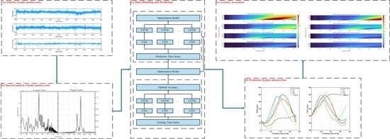
CNN and LSTM have unique characteristics in the process of time series prediction. CNN can extract and optimize features related to polar motion and LSTM can predict future data based on the long-term historical time series data. This section describes a hybrid CNN–LSTM model for polar motion prediction to improve the prediction accuracy. The polar motion prediction processes are divided into three main parts: data pre-processing, data modeling and prediction, and accuracy evaluation. As shown in Figure 4, the polar motion time series are entered in the first step and pre-processed by data normalization. Then, the polar motion time series are divided into two parts: the first part is used as training data to obtain an optimization model, and the second part is used as prediction data to obtain the polar motion time series by the optimization model. In the final experiment, accuracy indicators are used to evaluate the prediction model.

3.2. LS + AR Model

3.2.1. LS Model

To investigate the accuracy of the LS + AR model for predicting polar motion, it is necessary to separate the periodic and trend terms based on the LS method, considering that the polar motion series have mixed periodic and trend terms. The LS model is written as follows [16]:

$$X(t)=a+bt+{\displaystyle \sum _{i=1}^k{c}_i}\cos (\frac{2\pi t}{p_i}+{\omega }_i)+d_i\sin (\frac{2\pi t}{p_i}+{\omega }_i)$$

(13)

where $X(t)$ is the polar motion series; $a$ is a constant term; $b$ is a linear term; $c_i$ and $d_i$ are the coefficients for periodic terms; $p_i$ is the corresponding periodic; $k$ is the number of periodic terms; and ${\omega }_i$ is the phase of each periodic term.

The specific solution of the polar motion series of the LS model can be summarized as follows:

$$X=\left[\begin{array}{cccc}a& b& c_1& \begin{array}{ccc}{c}_2& d_1& \begin{array}{cc}{d}_2& \dots \end{array}\end{array}\end{array}\right]$$

(14)

$$B=\left[\begin{array}{cccc}1& t_1& \cos \frac{2\pi t_1}{p_1}& \begin{array}{cc}\sin \frac{2\pi t_1}{p_1}& \dots \end{array}\\ 1& t_2& \cos \frac{2\pi t_2}{p_2}& \begin{array}{cc}\sin \frac{2\pi t_2}{p_2}& \dots \end{array}\\ & & \dots & \begin{array}{cc}& \end{array}\\ 1& t_n& \cos \frac{2\pi t_n}{p_n}& \begin{array}{cc}\sin \frac{2\pi t_n}{p_n}& \dots \end{array}\end{array}\right]$$

(15)

$$X={(B^{T}B)}^{-1}{B}^{T}L$$

(16)

where $X$ is the estimated parameter vector; $B$ is the coefficient matrix; and $L$ is the observation vector.

3.2.2. AR Model

After modeling and predicting the deterministic part of the polar motion series, the remaining residuals are fitted to the prediction using an AR model, which is a prediction model based on past patterns of the time series variables themselves. The AR$(p)$ model equation for the fitted residual term of polar motion can be summarized as follows [48]:

$$Z_t={\displaystyle \sum _{i=1}^p{\phi }_i}{Z}_{t-i}+a_t$$

(17)

where ${\phi }_i$ is the model parameters, $a_t$ is the white noise, $Z_t$ is the fitted residual terms, and $p$ is the order of AR model.

3.3. Error Analysis

For verification of the prediction model, mean absolute error ($MAE$) and $RMSE$ were used to evaluate the predictive accuracy and objectivity of the results; they can be expressed as:

$$MAE=\frac{1}{n}{\displaystyle \sum _{i=1}^n\left|X_i-D_i\right|}$$

(18)

$$RMSE=\sqrt{\frac{{\displaystyle {\sum }_1^n{(X_i-D_i)}^2}}{n}}$$

(19)

where X_i is the predicted value of polar motion; $D_i$ is the corresponding observation value; $i$ is the span of time; and $n$ is the number of predictions.

3.4. Strategies for Polar Motion Prediction

3.4.1. Sources of Polar Motion Data

The IERS board of directors released the latest version of EOP 14C04 as an IERS reference series (United States Naval Observatory, Washington, DC, USA) on 1 February 2017 [49], which is available at https://hpiers.obspm.fr/eoppc/eop/eopc04/ (accessed on 30 September 2022). Figure 5 shows the polar motion provided by IERS from 1 January 1962 to the present (MJD: 37665-59793). The time span of this experiment is from 1 January 2009 to 31 December 2021.

3.4.2. Experimental Schemes

In this study, to examine the effects of different base time series on prediction accuracy, we designed five sets of prediction experiments using the EOP 14C04 series between 1 January 2009 and 31 December 2020. Furthermore, to explore the accuracy of the ERP series estimated by VLBI observations, we predicted the polar motion series based on the ERP series estimated from 2011 to 2020 VLBI observations. The prediction span was 360 days with one prediction per day, and the prediction period was from 1 January 2021 to 30 December 2021, for a total 360 predictions until the end of 2021. The following are the schemes of this experiments:

• Scheme 1: 1 January 2015 to 31 October 2020 was chosen as the 6-year base time series, with the LS + AR method used for prediction;
• Scheme 2: 1 January 2015 to 31 October 2020 was selected as the 6-year base time series, with the CNN–LSTM method used for prediction;
• Scheme 3: 1 January 2013 to 31 October 2020 was chosen as the 8-year base time series and the CNN–LSTM method is used for prediction;
• Scheme 4: 1 January 2011 to 31 October 2020 was selected as the 10-year base time series, with the CNN–LSTM method used prediction;
• Scheme 5: 1 January 2009 to 31 October 2020 was chosen as the 12-year base time series, with the CNN–LSTM method used for prediction;
• Scheme 6: Prediction of the polar motion series based on the ERP series estimated from 2011 to 2020 VLBI observations, with the CNN–LSTM method used for prediction.

Figure 6 shows the comparison of polar motion prediction in different schemes. The experiments we performed showed that the 12-year base time series fits the true value better and the fit becomes closer to the true value with increased base time series length; unexpectedly, the 6-year base time series was a poor match to the true value. Notably, in the current study we found that the prediction of polar motion based on the ERP series estimated from 2011 to 2020 VLBI observations has a better fit. The accuracy statistics of the prediction results are shown in

Table 5. Accuracy statistics of different prediction schemes (RMSE (mas)). Scheme 1 is a 6-year base time series prediction based on LS + AR model, Schemes 2–5 are base time series prediction based on hybrid CNN–LSTM model, and Scheme 6 is prediction of estimated polar motion from 2011 to 2020 VLBI observations based on hybrid CNN–LSTM model.

Parameters	Schemes	Time Span (d)
		1	5	10	20	30	40	60	90	120	180	270	360
PMX	1	0.23	2.16	3.04	6.86	10.37	11.17	19.37	24.67	30.58	32.07	34.63	39.43
	2	2.14	2.03	2.30	4.18	7.51	10.87	16.10	23.73	32.44	57.62	100.65	95.11
	3	1.93	2.40	3.35	5.31	5.00	4.36	6.96	17.47	32.50	46.41	41.91	37.71
	4	0.35	1.55	2.37	3.37	4.13	4.93	6.59	8.43	13.57	31.94	47.10	56.26
	5	0.61	1.22	1.37	1.37	1.48	1.43	1.46	4.33	6.35	11.34	19.68	18.01
	6	0.04	1.71	2.57	2.08	4.54	8.78	18.69	35.38	46.38	46.65	42.47	38.73
PMY	1	0.61	1.69	2.57	5.05	11.71	14.31	18.64	24.59	31.67	34.05	34.87	40.36
	2	0.21	0.39	2.13	5.69	5.54	5.07	6.49	18.03	23.82	22.39	62.25	109.30
	3	0.44	0.38	1.06	4.73	8.11	9.99	16.94	23.35	22.90	30.42	35.07	31.52
	4	0.86	1.34	2.75	7.71	10.89	12.14	16.42	18.83	17.12	45.05	59.21	60.17
	5	2.11	3.24	4.78	4.93	4.59	6.11	7.93	11.60	15.64	26.41	29.94	27.75
	6	4.24	5.36	7.28	10.76	14.97	20.57	27.11	31.68	29.76	26.93	22.90	20.39

. Scheme 2 had the lowest accuracy, which may be due to the poor training model caused by the short time series. It is notable that the hybrid CNN–LSTM model with 12-year base time series had the highest polar motion prediction accuracy; compared with the LS + AR model, especially in medium- to long-term prediction (90–360 days), and the accuracy of PMX and PMY was improved by about 54% and 31%, respectively. One unanticipated finding was that the accuracy of the ERP series estimated from 2011 to 2020 VLBI observations reached the level of the EOP 14C04 series in the medium- and long-term polar motion prediction for the same period, which also verifies that the ERP estimation experiment in this paper meets the requirement of high accuracy.

4. Discussion

The International VLBI Service for Geodesy and Astrometry (IVS) organized IVS-R1 and IVS-R4 sessions every Monday and Thursday, respectively, and these sessions usually involve a network of 5–10 VLBI stations for observation [13]. In this paper, the ERP series were obtained by estimating VLBI observations from 2011 to 2020 for IVS-R1/R4 sessions; furthermore, the CONT08, CONT11, CONT14, and CONT17 observations were estimated. The results show that the average RMSE based on the IVS-R1/R4 solution is about 0.19 mas for polar motion and 0.02 ms for UT1-UTC, while the accuracy of the CONT solutions is about 0.04 mas and 0.01 ms for polar motion and UT1-UTC, respectively. There may be two reasons for these results: One may be that the IVS-R1/R4 sessions have only 5–10 stations, while CONT campaigns have more globally distributed stations, and the IVS-R1/R4 sessions have a lower rate of data recording (256 Mbit/s) rather than the faster 512 Mbit/s. Another reason may be the difference in accuracy due to the epoch continuum.

Obviously, polar motion is one of the key parameters of ERP, which is defined as the motion of the Celestial Intermediate Pole (CIP) relative to the Earth’s surface. It is composed of a collection of motions covering a range from secular to sub-daily time scales [50]. The polar motion series consists of three significant components: long-term trend, Chandler wobble, and annual wobble. The large-scale secular deformation of Earth causes long-term drift of the polar motion [51]. The Chandler wobble refers to the motion of the CIP over the Earth’s surface, which is caused by the rotation axis not being aligned with the inertia axis [50], and is an excited resonance of the Earth’s rotation over a period of about 14 months [52]. The annual wobble is another important component of the polar motion and current findings confirm that it consists of two components, retrograde, and prograde wobble [53,54].

Furthermore, to explore the high-frequency variations in more detail, fast Fourier transform (FFT), for polar motion time series spectrum analysis, was selected in this paper. The spectrum of polar motion series is plotted in Figure 7, and the results show that the polar motion series exhibit extremely significant Chandler and annual wobble of about 426 days and 360 days, respectively. In addition, the results also showed a weaker retrograde oscillation with an amplitude of about 3.5 mas, and we enlarged the scale of the amplitude in order to explore more details of the retrograde wobble. Previous studies have proposed that the possible causes of excitation for Chandler wobble include variations in submarine, atmospheric, and groundwater pressure, as well as seismic excitation, and the annual wobble may be excited by variations in the atmosphere, ocean, and groundwater [55,56,57].

Moreover, a hybrid CNN–LSTM model is proposed in this paper, which is used for polar motion time series of prediction.

Table 6. Comparison of MAE for polar motion prediction based on two schemes. Hybrid CNN–LSTM model statistics represent the accuracy of the 12-year base time series.

Span (d)	Bulletin A		CNN–LSTM		Improvement
	PMX (mas)	PMY (mas)	PMX (mas)	PMY (mas)	PMX (%)	PMY (%)
1	0.19	0.51	0.61	2.11	−221.05	−313.72
5	0.79	1.62	0.91	2.32	−15.19	−43.21
10	1.11	2.03	1.09	2.79	1.80	−37.43
20	1.55	3.45	1.18	4.46	23.87	−29.28
30	3.34	4.34	1.32	4.13	60.48	4.84
40	5.24	6.67	1.25	5.40	76.15	19.63
90	12.80	11.07	2.99	10.19	22.54	7.95
180	11.40	25.84	8.83	22.36	22.56	13.47
270	18.94	29.93	15.85	26.79	16.31	10.50
360	24.45	28.71	14.03	24.99	42.62	12.96

shows the comparison of the MAE of Bulletin A and the 12-year polar motion prediction based on the hybrid CNN–LSTM model. Compared with Bulletin A, the results show that the accuracy of the hybrid CNN–LSTM model is slightly inferior in ultra-short-term polar motion prediction; this is because the model is being trained in the initial stage when it is less effective. However, the prediction accuracy gradually improved over time; notably, the prediction accuracy for PMX and PMY over a time span of 360 days improved by 42% and 13%, respectively. These results support the conclusion that the hybrid CNN–LSTM model can indeed improve the prediction accuracy of polar motion.

Figure 8 and Figure 9 show the mean absolute error (MAE) of 360-day polar motion prediction using the EOP 14C04 series for the period 1 January 2009 to 31 December 2020. PMX and PMY with 6-year base time series show large errors, especially for medium- to long-term prediction (180–360 days), which is mainly due to the poor training effect caused by the short time series. At the same time, we found that the 12-year base time series had the highest prediction accuracy, mainly due to the fact that the prediction accuracy can be optimized when the length of the base time series is sufficient.

5. Conclusions

Earth rotation parameters play a crucial role in high-precision timing services, precise orbiting of artificial satellites, etc. Prior studies have noted the importance of estimating and predicting ERP. We obtained the ERP series by estimating VLBI observations from 2011 to 2020 for IVS-R1/R4 sessions; furthermore, the CONT08, CONT11, CONT14, and CONT17 observations were estimated. The results show an average RMSE of 0.187 and 0.205 mas for PMX and PMY, respectively, and accuracy of 0.022 ms for UT1-UTC based on IVS-R1/R4 solutions. The accuracy of polar motion for CONT solutions was in the range of 0.03–0.05 mas, and for UT1-UTC based on the CONT solutions it was 0.005–0.01 ms.

Furthermore, to investigate the high-frequency variations in more detail, we performed spectral analysis of the polar motion series using fast Fourier transform (FFT). The results show that the polar motion series exhibit extremely significant Chandler and annual wobble of about 426 days and 360 days, respectively. In addition, the results also show weaker retrograde oscillation with an amplitude of about 3.5 mas.

Another important finding is that the hybrid CNN–LSTM model proposed in this paper is applicable to polar motion prediction. In short term prediction (0–60 days), the LS + AR model was superior, whereas in medium- to long-term prediction (90–360 days), the hybrid CNN–LSTM model improved PMX and PMY 54% and 31%, respectively. These results further support the observation that the hybrid CNN–LSTM model is slightly less accurate in short-term prediction and more accurate in medium- and long-term prediction. One possible explanation for these results is that the model may not have been trained optimally at the beginning. In addition, possible interference of the base time series cannot be ruled out. We tested the variability of the effect of different base series on the prediction of polar motion, and the results indicate that the accuracy of the prediction model gradually improved over time.

One limitation of the methods in this paper is that the training model for the 6-year base series was not very effective, and this needs to be further explored in our next work. We also need to consider the effect of numerous excitation sources on the prediction accuracy. Our future work will be devoted to investigating the effect of different excitation sources and base time series on prediction accuracy.

References

- Kalarus, M.; Schuh, H.; Kosek, W.; Akyilmaz, O.; Bizouard, C.; Gambis, D.; Gross, R.; Jovanović, B.; Kumakshev, S.; Kutterer, H.; et al. Achievements of the Earth orientation parameters prediction comparison campaign. J. Geod. 2010, 84, 587–596. [Google Scholar] [CrossRef]
- Herring, T.A.; Dong, D. Measurement of diurnal and semidiurnal rotational variations and tidal parameters of Earth. J. Geophys. Res. Solid Earth 1994, 99, 18051–18071. [Google Scholar] [CrossRef]
- Chen, J.L.; Wilson, C.R.; Eanes, R.J.; Tapley, B.D. A new assessment of long-wavelength gravitational variations. J. Geophys. Res. Solid Earth 2000, 105, 16271–16277. [Google Scholar] [CrossRef]
- Freedman, A.P.; Steppe, J.A.; Dickey, J.O.; Eubanks, T.M.; Sung, L.Y. The short-term prediction of universal time and length of day using atmospheric angular momentum. J. Geophys. Res. 1994, 99, 6981–6996. [Google Scholar] [CrossRef]
- Gambis, D. Monitoring Earth orientation using space-geodetic techniques: State-of-the-art and prospective. J. Geod. 2004, 78, 295–303. [Google Scholar] [CrossRef]
- Lambeck, K. The Earth’s Variable Rotation; Cambridge University Press: Cambridge, UK, 1980. [Google Scholar]
- Xu, C.; Shen, W.; Chao, D. Geophysical Geodesy Principles and Methods; Wuhan University Press: Wuhan, China, 2006. [Google Scholar]
- Böhm, S.; Brzeziński, A.; Schuh, H. Complex demodulation in VLBI estimation of high frequency Earth rotation components. J. Geodyn. 2012, 62, 56–68. [Google Scholar] [CrossRef]
- Dow, J.M.; Neilan, R.E.; Rizos, C. The International GNSS Service in a changing landscape of Global Navigation Satellite Systems. J. Geod. 2009, 83, 191–198. [Google Scholar] [CrossRef]
- Brzeziński, A. On estimation of high frequency geophysical signals in Earth rotation by complex demodulation. J. Geodyn. 2012, 62, 74–82. [Google Scholar] [CrossRef]
- Brzeziński, A.; Bizouard, C.; Petrov, S.D. Influence Of The Atmosphere On Earth Rotation: What New Can Be Learned From The Recent Atmospheric Angular Momentum Estimates? Surv. Geophys. 2002, 23, 33–69. [Google Scholar] [CrossRef]
- MacMillan, D.S. EOP and scale from continuous VLBI observing: CONT campaigns to future VGOS networks. J. Geod. 2017, 91, 819–829. [Google Scholar] [CrossRef]
- Nilsson, T.; Heinkelmann, R.; Karbon, M.; Raposo-Pulido, V.; Soja, B.; Schuh, H. Earth orientation parameters estimated from VLBI during the CONT11 campaign. J. Geod. 2014, 88, 491–502. [Google Scholar] [CrossRef]
- Puente, V.; Azcue, E.; Gomez-Espada, Y.; Garcia-Espada, S. Comparison of common VLBI and GNSS estimates in CONT17 campaign. J. Geod. 2021, 95, 120. [Google Scholar] [CrossRef]
- Akyilmaz, O.; Kutterer, H. Prediction of Earth rotation parameters by fuzzy inference systems. J. Geod. 2004, 78, 82–93. [Google Scholar] [CrossRef]
- Kosek, W.; Kalarus, M.; Niedzielski, T. Forecasting of the Earth orientation parameters—Comparison of different algorithms. Nagoya J. Med. Sci. 2008, 69, 155–158. [Google Scholar]
- Schuh, H.; Ulrich, M.; Egger, D.; Müller, J.; Schwegmann, W. Prediction of Earth orientation parameters by artificial neural networks. J. Geod. 2002, 76, 247–258. [Google Scholar] [CrossRef]
- Jin, X.; Liu, X.; Guo, J.; Shen, Y. Analysis and prediction of polar motion using MSSA method. Earth Planets Space 2021, 73, 147. [Google Scholar] [CrossRef]
- Kiani Shahvandi, M.; Schartner, M.; Soja, B. Neural ODE Differential Learning and Its Application in Polar Motion Prediction. J. Geophys. Res. Solid Earth 2022, 127, e2022JB024775. [Google Scholar] [CrossRef]
- Akyilmaz, O.; Kutterer, H.; Shum, C.K.; Ayan, T. Fuzzy-wavelet based prediction of Earth rotation parameters. Appl. Soft Comput. 2011, 11, 837–841. [Google Scholar] [CrossRef]
- Kosek, W.; McCarthy, D.D.; Luzum, B.J. El Niño Impact on Polar Motion Prediction Errors. Stud. Geophys. Geod. 2001, 45, 347–361. [Google Scholar] [CrossRef]
- Niedzielski, T.; Kosek, W. Prediction of UT1–UTC, LOD and AAM χ3 by combination of least-squares and multivariate stochastic methods. J. Geod. 2007, 82, 83–92. [Google Scholar] [CrossRef]
- Chin, T.M.; Gross, R.S.; Dickey, J.O. Modeling and forecast of the polar motion excitation functions for short-term polar motion prediction. J. Geod. 2004, 78, 343–353. [Google Scholar] [CrossRef]
- Gambis, D.; Salstein, D.A.; Lambert, S. Use of atmospheric angular momentum forecasts for UT1 predictions: Analyses over CONT08. J. Geod. 2011, 85, 435–441. [Google Scholar] [CrossRef]
- Su, X.; Liu, L.; Houtse, H.; Wang, G. Long-term polar motion prediction using normal time–Frequency transform. J. Geod. 2013, 88, 145–155. [Google Scholar] [CrossRef] [Green Version]
- Li, P.; Abdel-Aty, M.; Yuan, J. Real-time crash risk prediction on arterials based on LSTM-CNN. Accid. Anal. Prev. 2020, 135, 105371. [Google Scholar] [CrossRef] [PubMed]
- Tian, C.; Ma, J.; Zhang, C.; Zhan, P. A Deep Neural Network Model for Short-Term Load Forecast Based on Long Short-Term Memory Network and Convolutional Neural Network. Energies 2018, 11, 3493. [Google Scholar] [CrossRef] [Green Version]
- Xia, W.; Zhu, W.; Liao, B.; Chen, M.; Cai, L.; Huang, L. Novel architecture for long short-term memory used in question classification. Neurocomputing 2018, 299, 20–31. [Google Scholar] [CrossRef]
- Karim, F.; Majumdar, S.; Darabi, H.; Chen, S. LSTM Fully Convolutional Networks for Time Series Classification. IEEE Access 2018, 6, 1662–1669. [Google Scholar] [CrossRef]
- Zhou, H.; Sun, J.; Zhao, Z.; Yang, Y.; Xie, A.; Chiclana, F. Attention-Based Deep Learning Model for Predicting Collaborations Between Different Research Affiliations. IEEE Access 2019, 7, 118068–118076. [Google Scholar] [CrossRef]
- Böhm, J.; Böhm, S.; Nilsson, T.; Pany, A.; Plank, L.; Spicakova, H.; Teke, K.; Schuh, H. The New Vienna VLBI Software VieVS. In Geodesy for Planet Earth; Springer: Berlin/Heidelberg, Germany, 2012; pp. 1007–1011. [Google Scholar]
- Böhm, J.; Böhm, S.; Boisits, J.; Girdiuk, A.; Gruber, J.; Hellerschmied, A.; Krásná, H.; Landskron, D.; Madzak, M.; Mayer, D.; et al. Vienna VLBI and Satellite Software (VieVS) for Geodesy and Astrometry. Publ. Astron. Soc. Pac. 2018, 130, 044503. [Google Scholar] [CrossRef]
- Kalarus, M.; Kosek, W.; Schuh, H. Current Results of the Earth Orientation Parameters Prediction Comparison Campaign; Observatoire de Paris: Paris, France, 2007. [Google Scholar]
- Ros, C.T.; Pavetich, P.; Nilsson, T.; Böhm, J.; Schuh, H. Vienna SAC-SOS: Analysis of the European Vlbi Sessions. In Proceedings of the IVS 2012 General Meeting Proceedings “Launching the Next-Generation IVS Network”, Madrid, Spain, 4–9 March 2012. [Google Scholar]
- Petit, G. Relativity in the IERS Conventions. Proc. Int. Astron. Union 2010, 5, 16–21. [Google Scholar] [CrossRef] [Green Version]
- Altamimi, Z.; Rebischung, P.; Métivier, L.; Collilieux, X. ITRF2014: A new release of the International Terrestrial Reference Frame modeling nonlinear station motions. J. Geophys. Res. Solid Earth 2016, 121, 6109–6131. [Google Scholar] [CrossRef]
- Gordon, D. Impact of the VLBA on reference frames and earth orientation studies. J. Geod. 2016, 91, 735–742. [Google Scholar] [CrossRef]
- Landskron, D.; Böhm, J. VMF3/GPT3: Refined discrete and empirical troposphere mapping functions. J. Geod. 2018, 92, 349–360. [Google Scholar] [CrossRef]
- Blakemore, D. Relevance and Linguistic Meaning: The Semantics and Pragmatics of Discourse Markers; Cambridge University Press: Cambridge, UK, 2002. [Google Scholar]
- Bonn, U.u.L. Ensemble Simulations of Atmospheric Angular Momentum and Its Influence on the Earth’s Rotation. Doctoral Dissertation, Universitäts-und Landesbibliothek Bonn, Bonn, Germany, 2009. [Google Scholar]
- Montesinos López, O.A.; Montesinos López, A.; Crossa, J. Convolutional Neural Networks; Springer International Publishing: Cham, Switzerland, 2022; pp. 533–577. [Google Scholar]
- Zang, H.; Liu, L.; Sun, L.; Cheng, L.; Wei, Z.; Sun, G. Short-term global horizontal irradiance forecasting based on a hybrid CNN-LSTM model with spatiotemporal correlations. Renew. Energy 2020, 160, 26–41. [Google Scholar] [CrossRef]
- Zhao, J.; Mao, X.; Chen, L. Speech emotion recognition using deep 1D & 2D CNN LSTM networks. Biomed. Signal Process. Control 2019, 47, 312–323. [Google Scholar] [CrossRef]
- Abdeljaber, O.; Avci, O.; Kiranyaz, S.; Gabbouj, M.; Inman, D.J. Real-time vibration-based structural damage detection using one-dimensional convolutional neural networks. J. Sound Vib. 2017, 388, 154–170. [Google Scholar] [CrossRef]
- Li, T.; Hua, M.; Wu, X. A Hybrid CNN-LSTM Model for Forecasting Particulate Matter (PM2.5). IEEE Access 2020, 8, 26933–26940. [Google Scholar] [CrossRef]
- Liu, H.; Mi, X.-w.; Li, Y.-f. Wind speed forecasting method based on deep learning strategy using empirical wavelet transform, long short term memory neural network and Elman neural network. Energy Convers. Manag. 2018, 156, 498–514. [Google Scholar] [CrossRef]
- Gers, F.A.; Schmidhuber, J.; Cummins, F. Learning to Forget: Continual Prediction with LSTM. Neural Comput. 2000, 12, 2451–2471. [Google Scholar] [CrossRef]
- Young, P.; Shellswell, S. Time series analysis, forecasting and control. IEEE Trans. Autom. Control 1972, 17, 281–283. [Google Scholar] [CrossRef]
- Bizouard, C.; Lambert, S.; Gattano, C.; Becker, O.; Richard, J.-Y. The IERS EOP 14C04 solution for Earth orientation parameters consistent with ITRF 2014. J. Geod. 2018, 93, 621–633. [Google Scholar] [CrossRef]
- McCarthy, D.D.; Seidelmann, P.K. Time: From Earth Rotation to Atomic Physics; Cambridge University Press: Cambridge, UK, 2018. [Google Scholar]
- King, M.A.; Watson, C.S. Geodetic vertical velocities affected by recent rapid changes in polar motion. Geophys. J. Int. 2014, 199, 1161–1165. [Google Scholar] [CrossRef] [Green Version]
- Gross, R. The excitation of the Chandler wobble. Geophys. Res. Lett. 2000, 27, 2329–2332. [Google Scholar] [CrossRef] [Green Version]
- King, N.E.; Agnew, D.C. How large is the retrograde annual wobble. Geophys. Res. Lett. 1991, 18, 1735–1738. [Google Scholar] [CrossRef]
- Schindelegger, M.; Böhm, J.; Salstein, D.; Schuh, H. High-resolution atmospheric angular momentum functions related to Earth rotation parameters during CONT08. J. Geod. 2011, 85, 425–433. [Google Scholar] [CrossRef]
- Min, Z.; Haoming, Y.; Yaozhong, Z. The investigation of atmospheric angular momentum as a contributor to polar wobble and length of day change with AMIP II GCM data. Adv. Atmos. Sci. 2002, 19, 287–296. [Google Scholar] [CrossRef]
- Höpfner, J. Low-Frequency Variations, Chandler and Annual Wobbles of Polar Motion as Observed Over One Century. Surv. Geophys. 2004, 25, 1–54. [Google Scholar] [CrossRef] [Green Version]
- Gross, R.; Fukumori, I.; Menemenlis, D. Atmospheric and Oceanic Excitation of the Earth’s Wobbles During 1980–2000. J. Geophys. Res. Solid Earth 2003, 108, B8. [Google Scholar] [CrossRef]
Figure 1.
Flow diagram of geodetic VLBI observations analysis.
Figure 2.
Daily solutions of residual polar motion and UT1-UTC based on VLBI observations from 2011 to 2020 after subtracting daily ERP series provided by IERS; PMX, PMY represent the x and y components of polar motion series respectively, UT1-UTC is universal time.
Figure 3.
Network architecture of LSTM.
Figure 4.
Flowchart of polar motion prediction using hybrid CNN–LSTM model.
Figure 5.
Polar motion time series from 1 January 1962 to now (MJD: 37665-59793); PMX, PMY represent the x and y components of polar motion series respectively.
Figure 6.
Comparison of polar motion prediction in different base time series based on hybrid CNN–LSTM model. True value was provided by Bulletin A. In graphs, 6y–12y indicate predicted values for different base time series and VLBI-10y is the VLBI observations estimated in this paper.
Figure 7.
Spectral analysis of polar motion series: retrograde wobble (left) and prograde wobble (right); scale of amplitude of left graph is enlarged to explore retrograde wobble in more detail.
Figure 8.
MAE (unit: mas) of PMX prediction using hybrid CNN–LSTM model based on different base time series.
Figure 9.
MAE (unit: mas) of PMY prediction using hybrid CNN–LSTM model based on different base time series.