
SRTM DEM Correction Using Ensemble Machine Learning Algorithm
1
College of Science, Central South University of Forestry and Technology, Changsha 410001, China
2
School of Earth Science and Spatial Information Engineering, Hunan University of Science and Technology, Xiangtan 411201, China
3
School of Geosciences and Info-Physics, Central South University, Changsha 410083, China
4
Hunan Engineering and Research Center of Natural Resource Investigation and Monitoring, Changsha 410007, China
*
Author to whom correspondence should be addressed.
Remote Sens. 2023, 15(16), 3946; https://doi.org/10.3390/rs15163946
Submission received: 20 June 2023
/
Revised: 1 August 2023
/
Accepted: 2 August 2023
/
Published: 9 August 2023
(This article belongs to the Special Issue Remote Sensing Data Fusion and Applications)
Abstract
:The Shuttle Radar Topographic Mission (SRTM) digital elevation model (DEM) is a widely utilized product for geological, climatic, oceanic, and ecological applications. However, the accuracy of the SRTM DEM is constrained by topography and vegetation. Using machine learning models to correct SRTM DEM with high-accuracy reference elevation observations has been proven to be useful. However, most of the reference observation-aided approaches rely on either parametric or non-parametric regression (e.g., a single machine learning model), which may lead to overfitting or underfitting and limit improvements in the accuracy of SRTM DEM products. In this study, we presented an algorithm for correcting SRTM DEM using a stacking ensemble machine learning algorithm. The proposed algorithm is capable of learning how to optimally combine the predictions from multiple well-performing machine learning models, resulting in superior performance compared to any individual model within the ensemble. The proposed approach was tested under varying relief and vegetation conditions in Hunan Province, China. The results indicate that the accuracy of the SRTM DEM productions improved by approximately 46% using the presented algorithm with respect to the original SRTM DEM. In comparison to two conventional algorithms, namely linear regression and artificial neural network models, the presented algorithm demonstrated a reduction in root-mean-square errors of SRTM DEM by 28% and 12%, respectively. The approach provides a more robust tool for correcting SRTM DEM or other similar DEM products over a wide area.
1. Introduction
A digital elevation model (DEM) is a three-dimensional representation of bare topographic surfaces created through digital means [1]. DEMs are essential for various applications in fields such as topography, geology, geomorphology, hydrology, and ecology [2], as they allow for the characterization, monitoring, and analysis of changes to the Earth’s surface in three dimensions [3]. Due to the increasing demand for DEMs [4], a range of freely available global or near-global DEMs have been produced over the past two decades, including the Shuttle Radar Topography Mission (SRTM) DEM [5], Advanced Spaceborne Thermal Emission and Reflection Radiometer (ASTER) DEM [6], Advance Land Observing Satellite (ALOS) world 3D-30 m (AW3D30) DEM [7], and the Copernicus DEM [8]. These DEM products were obtained through various remote sensing techniques. For example, the ASTER DEM and AW3D30 DEM were both generated using the space-based optical stereo matching technique, whereas the SRTM DEM and Copernicus DEM were generated using space-borne interferometric synthetic aperture radar (InSAR) techniques. Among the global DEMs, the SRTM DEM is widely utilized due to its extensive coverage from 60°N to 57°S [9], open accessibility, and early release date in February 2003. However, according to [10], SRTM DEM contains error biases of up to 3.6 m and large uncertainties of up to 16.16 m in vegetated areas or areas with steep topography. It has been demonstrated that an effective method to correct SRTM DEM errors involves the utilization of high-quality auxiliary elevation observations obtained from ground-based leveling benchmarks, GPS receivers, LiDAR, and ice, cloud, and land elevation satellites (ICESat). Consequently, numerous algorithms have been developed in recent years to facilitate the correction of the error of the SRTM DEM. These algorithms can be roughly categorized into two groups based on the models employed, namely parametric regression and non-parametric regression. The former aims to model and eliminate DEM error trends by fitting SRTM DEM deviations with error-related variables derived from high-quality auxiliary elevation observations (e.g., canopy cover, slope, aspect, elevation height, vegetation height, and density) [11,12,13,14,15,16,17,18,19,20,21,22,23,24]. In addition to the quality of collected reference elevation observations, such as their number, density, and accuracy, the performance of SRTM DEM correction using parametric regression algorithms primarily depends on the fit of the mathematical models. Theoretically, incorporating more variables related to SRTM DEM errors into these models is beneficial to better describe complicated error patterns. However, the inclusion of additional input variables may result in the curse of dimensionality, particularly in areas with highly nonlinear error patterns [25], which significantly restricts the practical applications of parametric regression algorithms.
The second category of SRTM DEM correction involves non-parametric machine learning algorithms. For example, Ref. [26] proposed the use of an artificial neural network (ANN) to correct SRTM DEMs. Their approach involved generating a training model based on 11 bands of Landsat-8 multispectral imagery and highly accurate reference elevation data. Their results indicated an average improvement in accuracy of approximately 55% for two test sites. Compared to parametric regression algorithms, machine learning algorithms do not require specific assumptions about the mapping function between DEM errors and the related variables. Therefore, if suitable training samples are available, machine learning algorithms can theoretically describe and correct complex error patterns in SRTM DEM. In recent years, several enhanced machine learning-based algorithms have been developed to improve the accuracy of predictions. These include incorporating additional variables [25] and utilizing other ANN algorithms, such as multilayer perceptron neural networks, fully convolutional neural networks, random forests, and multi-channel convolutional neural networks, among others [25,27,28,29,30,31,32]. However, the majority of existing studies employ a single machine learning model to correct SRTM DEM errors, resulting in poor robustness. Specifically, for the same or slightly different training samples, the same machine learning algorithm produces varying prediction outputs each time. Additionally, different machine learning algorithms yield distinct predictions.
Ensemble learning algorithms involve training multiple machine learning models and combining their predictions to improve accuracy and robustness [33,34]. Numerous studies have demonstrated the superior accuracy and robustness of ensemble learning algorithms compared to any single machine learning model involved in the ensemble, as evidenced by research in image classification, data mining, and numerical prediction [35,36,37]. Meanwhile, ensemble methods have gained widespread adoption in terrain characterization and digital elevation model research [20,23,24]. For instance, Shastry et al. [20] enhanced the precision of a digital elevation model for flood simulation through the application of ensemble data assimilation techniques. Due to this advantage, utilizing ensemble learning algorithms instead of a single machine learning model, as used in previous studies, can improve the level of accuracy and correct SRTM DEM errors. However, to the best of our knowledge, few studies on correcting SRTM DEM errors using ensemble learning algorithms have been presented so far. Therefore, in this paper, we propose a framework for correcting these errors with the assistance of high-quality auxiliary elevation observations. We refer to this framework as the Stacking Fusion Correction Model (SFCM). This paper is organized as follows. Section 2 introduces the study area and dataset, followed by a description of the methods used to correct SRTM DEM errors using an ensemble learning framework. The results and discussions are presented in Section 4, while Section 5 provides conclusions and prospects.
2. Study Areas and Datasets
2.1. Study Areas
In this study, the SFCM algorithm was tested in four regions in Hunan Province, namely Chenzhou, Yongzhou, Yueyang, and Changde (see Figure 1b), China. The total area of these four regions is approximately 74,845 km2. The Chenzhou and Yongzhou regions are situated in the southern part of Hunan Province and are delineated by cyan and red lines in Figure 1b. These areas are characterized by the Luoxiao Mountains and Nanling Mountains, which create a dramatic variation in terrain with elevations ranging from 28 m to 2040 m and slopes changing from 0° to 73° (see Figure 1c,d). The Yueyang and Changde regions, delineated by cyan and red lines in Figure 1b, are situated in the northern part of Hunan province with elevations ranging from 12 m to 2060 m and terrain slopes varying from 0° to 75° (see Figure 1e,f). The mean slope of the Yueyang and Changde regions is approximately 8.5°, which is lower than that of the selected Chenzhou and Yongzhou regions, whose average slope measures around 14.7°.
As depicted in Figure 1b, the four selected regions exhibit diverse surface covers, including forests, grasslands, wetlands, cultivated lands, artificial surfaces, and bare earth. This enables us to evaluate the performance of the SFCM algorithm across different land cover types. In Table 1, it is evident that the mean canopy height in the Chenzhou (8.1 m) and Yongzhou (7.5 m) regions are almost equivalent to each other, surpassing those of the Yueyang (5.6 m) and Changde (5.8 m) regions. Additionally, the average vegetation coverage in Chenzhou (71.8%) is approximately equivalent to that of Yongzhou (70.2%), both of which exceed that of the Yueyang (59.4%) and Changde regions (58.7%). In terms of overall terrain characteristics and surface coverage, Chenzhou is similar to Yongzhou, while Yueyang resembles Changde. Therefore, we utilized datasets from the Chenzhou and Changde regions as training data while employing datasets from the Yongzhou and Yueyang regions for testing purposes to validate our proposed algorithm.
2.2. Datasets
2.2.1. SRTM DEM
SRTM (Shuttle Radar Topography Mission) was a radar topography mission conducted by the space shuttle Endeavor in February 2000 [5], which acquired elevation data from 56°S to 60°N of the global land surface [38]. The SRTM DEM products are available in resolutions of 90 m and 30 m, with a horizontal datum of WGS84 and an elevation datum of EGM96. Since its initial public release in 2003, the SRTM DEM has undergone multiple revisions, resulting in several data versions being available. The first version, SRTM3 V1, was released by the National Aeronautics and Space Administration (NASA) on a continental basis but contained numerous voids and anomalous values while lacking any oceanic elevation data [5]; SRTM3 V2 was released by NASA in 2005 to address the gap region of SRTM3 V1 through spatial interpolation methods, which effectively mitigated water noise [39]. Subsequently, the Consortium of International Agricultural Research Centers (CGIAR) released SRTM3 V3 in 2006, which utilized the Global Waters Boundary Dataset to crop the shorelines and flatten waters. The gaps in SRTM3 V2 were filled using interpolation based on auxiliary data (e.g., GTOPO30, NED DTM, and ASTER DEMs) [40]; SRTM3 V4, which was released by the CGIAR in 2008, employs a novel interpolation algorithm [41] and addresses data gaps present in SRTM3 V3 with the aid of high-resolution DEMs such as Canadian Digital Elevation Data Level 1 [40]. In contrast to previous versions, SRTM1 was launched by the United States Geological Survey (USGS) in 2014 with significantly fewer voids, rendering it the highest resolution and most consistently high-quality SRTM DEM available; however, it still contains voids and outliers [42]. Compared to SRTM3, SRTM1 offers higher resolution and accuracy, enabling the extraction of more precise topographic information. Additionally, these data are more practical for calibration purposes. Therefore, in this paper, we have selected the SRTM1 DEM version obtained from (http://earthexplorer.usgs.gov/) (accessed on 8 October 2022).
2.2.2. Reference Elevation Data
In this study, two types of high-quality auxiliary elevation datasets were employed as reference elevation observations for SRTM DEM correction. The first dataset was obtained through the Global Navigation Satellite System (GNSS) with the assistance of Hunan Province’s Continuously Operating Reference Station (CORS) network. The CORS network comprises over 120 base stations (as of 2018) that facilitate the correction of common errors between base and rover receivers [43], thereby improving the post-processed coordinate accuracies of rover receivers to approach centimeter-level precision in both the vertical and horizontal dimensions [44,45]. To rectify errors in the SRTM DEM, we gathered a total of 742,007 GNSS observations from the CORS network located in Hunan province’s four selected regions (refer to Table 1 for further details).
The other type of high-quality auxiliary elevation dataset was acquired through the utilization of ICEsat-2 (Ice, Cloud, and Land Elevation Satellite). Launched in 2018, ICESat-2 represents the second generation of laser altimeter technology following the ICESat mission [46]. The Advanced Topographic Laser Altimeter System (ATLAS) employs multi-beam micropulse laser technology, emitting a single beam with a wavelength of 532 nm at an exceptionally high frequency of 10 kHz [47]. Each laser pulse transmitted is split by diffractive optics in the ATLAS, resulting in six separate beams arranged into three groups. Each group consists of strong and weak beams with an energy ratio of approximately 4:1, enabling continuous ground observation [48]. The ATL08 product generated from ICESat-2 acquisition provides highly accurate ground elevation data and vegetation canopy data, with vertical accuracy ranging from several centimeters to a few meters (e.g., below 3 m), depending on the evaluated areas and reference elevation samples [47,49]. This level of accuracy surpasses that of the SRTM DEM product. Therefore, we collected a total of 42,500 ATL08 elevation observations for our selected four study regions between 2019 to 2022 as an auxiliary elevation dataset to correct the SRTM DEM. The locations of the selected ATL08 elevation observations (https://search.earthdata.nasa.gov/) (accessed on 15 October 2022) are indicated by pink cycles in Figure 1c–f.
For the purpose of this work, we have designed the collected CORS GNSS and ICESat-2 ATL08 elevation observations as reference elevations. To ensure high-quality reference elevation data, we have eliminated significant errors exceeding a difference of 50 m between the reference elevations and corresponding SRTM DEM elevations [50]. This resulted in a total of 364,635 reference elevations for the two training regions (Yongzhou and Yueyang) and 419,872 reference elevations in the two testing regions (Chenzhou and Changde).
2.2.3. Ancillary Data
As indicated by previous studies [12,13,14,25,51], the accuracy of SRTM DEM products is closely associated with canopy height, vegetation coverage, and surface cover type. Therefore, we initially acquired the 2019 canopy height dataset provided by [52] at a resolution of 30 m. The canopy height dataset was generated through the fusion of Global Ecosystem Dynamics Investigation (GEDI), ICESat-2 ATLAS, and Sentinel-2 images using neural network-guided interpolation [52]. This resulted in a spatial resolution of 30 m and an accuracy level of 5 m (as denoted by standard deviation).
Additionally, vegetation coverage data obtained from the inversion of the normalized difference vegetation index for 2021 (https://modis.gsfc.nasa.gov/data/) (accessed on 18 December 2022) were also collected. The original resolution of the collected vegetation coverage data was 250 m, which was resampled to 30 m using the approach described by [53] to match the spatial resolution of the collected SRTM DEM. Finally, GlobalLand30 2020 data (http://www.globallandcover.com/) (accessed on 21 November 2022), a surface cover-type dataset with a resolution of 30 m and an accuracy level of 80% [54], were obtained.
3. Method
The ensemble learning algorithm combines predictions from multiple machine learning algorithms to produce an optimal predictive model, enhancing prediction robustness beyond that of a single machine learning algorithm. The models used in ensemble learning can be divided into two categories: base models consisting of multiple machine learning algorithms and meta-models that combine the predictions of the base models to produce an optimal result. In this study, we developed an ensemble learning framework for accurately correcting SRTM DEM data with the primary objective of improving correction accuracy. The base models in the constructed framework consist of random forest, extreme gradient boosting (XGBoost), light gradient boosting machine (LightGBM), and an ANN, with linear regression selected as the meta-model. The developed ensemble learning framework was employed to refine SRTM DEM using the collected ancillary data.
3.1. Stacking Fusion Correction Model (SFCM) Construction
3.1.1. Base Models of the SFCM
The accuracy improvement achieved by ensemble learning over an individual machine learning algorithm can be primarily attributed to two operations performed by the base models: (i) bagging, which reduces prediction variance by randomly sub-sampling the original dataset and independently training on each sub-sample, and (ii) boosting, which reduces prediction bias through iterative reweighting of the original datasets. In recent decades, a plethora of bagging and boosting algorithms have been developed. Theoretically, any combination of two or more algorithms can be selected as base models; however, the accuracy of different combinations may vary [55]. Among these algorithms, random forest is widely used for its ability to handle large datasets and provide higher predictive accuracy compared to decision tree algorithms. The extreme gradient boosting (XGBoost) algorithm and the light gradient boosting machine (LightGBM) are two advanced boosting algorithms that efficiently handle large datasets, generate highly accurate predictions, and exhibit good resistance to overfitting. These merits make them preferable base models for reducing variance and bias in SRTM DEM correction alongside the random forest algorithm [56,57,58]. Furthermore, artificial neural networks (ANN) exhibit a remarkable capacity for capturing nonlinear patterns in sample datasets while maintaining a high degree of robustness against data errors [59]. As such, this study incorporates an ANN into the base models to enhance prediction heterogeneity.
3.1.2. Meta-Models of the SFCM
As illustrated in Figure 2, the base models generated predictions based on all training datasets, and each selected model produced a distinct prediction due to varying training strategies. To address this issue, the stacking (or stacked generalization) technique was employed to integrate the predictions from multiple base learning models using a meta-learning model. In light of this, the base models are denoted as level 0 models, while the meta-model is referred to as a level 1 model. The meta-model initiates training and determines the optimal combination of predictions from multiple base models by minimizing a user-defined loss function. Specifically, the meta-model learns a weight vector denoting the significance of base learners according to the defined loss function, with larger weights implying a greater influence on the final prediction. It then multiplies each base learner’s prediction by its weight and sums them to obtain the final prediction. By quantifying each base learner’s contribution through the weighting mechanism of the meta-model, the prediction accuracy of the ensemble is enhanced. Therefore, the meta-model is typically a highly interpretable model, such as a decision tree, linear regression model, logistic regression model, and so on [60,61]. In this study, we selected linear regression as the meta-model for SFCM due to its simplicity, strong interpretability, and robustness. Additionally, we defined a loss function using the mean squared error (MSE), i.e.,
where represents the prediction of the -th base model, is the prediction of the meta-model, and n is the number of the selected base models.
3.1.3. SRTM DEM Correction Using SFCM
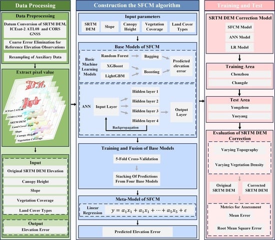
The SFCM procedure for correcting SRTM DEM is described in detail below. As illustrated in Figure 3, firstly, training datasets (including SRTM DEM products, reference elevation data, and the ancillary data listed in Section 2.2.3) were prepared, and parameters such as SRTM elevation, slope, surface cover type, canopy height, and vegetation coverage were input into four selected based models: random forest, XGBoost, LightGBM, and an ANN. Secondly, each of the selected base models underwent training on the training datasets through a 5-fold cross-validation process. The primary objective of utilizing this technique was to evaluate the proficiency of base models in handling new data and generate novel features that can expand the input samples for the meta-model [62]. In each iteration of the 5-fold cross-validation, the training dataset was randomly partitioned into five folds with approximately equal sizes. Each unique fold served as a validation set, while the remaining four folds were used for training. Each base model was trained on the training datasets for each combination of the 5-fold cross-validation, and its training performance was evaluated on the split validation set. As a result, five predictions were generated from each base model, which were then used as inputs to the meta-model to produce a final prediction using weighted linear regression. After obtaining the training model of the constructed ensemble learning algorithm, it was theoretically possible to correct SRTM DEM products outside of the training regions based on this model (as depicted in Equation (2)).
As indicated in Table 1, the terrain characteristics, canopy height, and vegetation cover exhibit similar averages between the Changde and Yueyang regions. Similarly, comparable averages are observed for the terrain characteristics, canopy height, and vegetation cover between the Chenzhou and Yongzhou regions. Therefore, we designated the Changde and Chenzhou regions as training areas while reserving the remaining two regions for validation purposes in order to optimize the ensemble learning algorithm’s training model generation. Specifically, we utilized CORS GNSS and ICESat-2 ATL08 elevation datasets collected from the Changde and Chenzhou regions as reference elevations to estimate errors present within SRTM DEM products. Then, the canopy height, vegetation coverage, elevation, slope, and land cover types of the Changde and Chenzhou regions were selected as training datasets in response to the estimated errors of SRTM DEM products. To mitigate the impact of gross errors, samples with estimated absolute errors larger than 50 m were filtered from the training datasets. It should be noted that the accuracy of SRTM DEM correction is evaluated using mean error (ME) and root-mean-square error (RMSE), as previously described by [9,63,64].
where represents the elevation values of SRTM DEM products, denotes the corresponding reference elevation data, and represents the total count of such reference data points.
4. Results and Discussion
4.1. SFCM-Based SRTM DEM Correction
Figure 4 illustrates both the original SRTM DEM and its corresponding SFCM-corrected version over these two test areas. The differences between the two are illustrated in Figure 4c,f for comparative analysis. As depicted in Figure 4, SRTM DEM has apparent errors in regions with complex terrains. More specifically, the root-mean-square error (RMSE) increases from 12.6 m to 17.3 m in the Yongzhou region and from 8.7 m to 15.6 m in the Yueyang region when slopes range between 0° and 30°; similarly, when elevations range between 0 m and 1500 m, the RMSE increases from 6.5 m to 14.4 m in the Yongzhou region and from 5.l m to 11.7 m in the Yueyang region. Additionally, the precision of SRTM DEM in non-vegetated regions is significantly superior to that in vegetated areas. As vegetation coverage increases from 0% to 100%, the root-mean-square error (RMSE) rises from 7.0 m to 13.6 m in the Yongzhou region and from 6.7 m to 10.5 m in the Yueyang region.
4.2. Accuracy Evaluation of the SFCM-Corrected SRTM DEMs
Figure 5 displays scatter plots depicting the correlation between the in situ reference elevations and the corresponding corrected SRTM DEMs across the Yueyang and Yongzhou regions. The SFCM-corrected SRTM DEM exhibits a favorable agreement with the in situ reference observations, as depicted in Figure 5. Specifically, for the Yueyang region, the mean error (ME) and root-mean-square error (RMSE) are approximately 0.01 m and 5.4 m, respectively, while for the Yongzhou region, they are about 0.01 m and 7.3 m. In addition, we conducted a linear regression analysis to establish the relationship between in situ reference elevations and the corresponding corrected SRTM DEM. The results indicate that the intercepts and slopes of the fitted linear functions (indicated by lines in Figure 5) for both the Yueyang and Yongzhou regions are close to zero and one, respectively, with coefficients of determination (R2) of 0.99 and 0.98 for the Yueyang and Yongzhou regions.
4.3. Performance Comparisons between the SFCM and the Classical Algorithms
As mentioned in Section 1, methods for correcting SRTM DEM based on in situ reference elevations can be broadly classified into two categories: parametric regression and non-parametric machine learning. In this section, we compared the performance of the presented SFCM algorithm with two classical algorithms for SRTM DEM correction, specifically linear regression (LR) [14], which belongs to the parametric regression group, and the ANN model [65], which belongs to the non-parametric machine learning group.
4.3.1. Comparison of Overall Accuracy
Figure 6b–d illustrates the histograms depicting the disparities between in situ elevations and SRTM DEMs, which have been rectified by employing the proposed SFCM, ANN, and LR algorithms across the Yongzhou region. Additionally, a histogram comparing the differences between the in situ elevations and the original SRTM DEM was presented in Figure 6a. The MEs and RMSEs of these discrepancies are displayed in Figure 6. As depicted by Figure 6, due to the presence of dense vegetation and mountainous terrain, the original SRTM DEM exhibits an ME and RMSE of 5.9 m and 13.4 m over the Yongzhou region. This indicates that the original SRTM DEM contains significant bias (as indicated by ME) and high variance (as denoted by RMSE), leading to errors. Fortunately, the utilization of the SFCM, ANN, and LR algorithms effectively mitigated bias and variance with varying degrees of accuracy. Specifically, these algorithms reduced the original bias of 5.91 m to 0.01 m, −0.05 m, and −0.06 m, respectively. However, the SFCM-corrected SRTM DEM exhibits a slightly smaller ME compared to the corrected SRTM DEMs generated by the other two algorithms. Furthermore, all three algorithms are capable of reducing the original RMSE of 13.4 m in the SRTM DEM to 7.3 m, 9.0 m, and 10.8 m for the SFCM, ANN, and LR algorithms, respectively. Compared to the existing ANN and LR algorithms, the SFCM-corrected SRTM DEM exhibits an RMSE that is smaller by 18.8% and 32.4%, respectively.
Figure 7 depicts the histograms illustrating the differences between the in situ elevations and the original, SFCM-corrected, ANN-corrected, and LR-corrected SRTM DEMs across the Yueyang region. As depicted in Figure 7a, the SRTM DEM still exhibits errors with a mean error of approximately 1.5 m and a root-mean-square error of 9.9 m. Due to the coarser resolution and lower vegetation cover in the Yueyang region, both the bias and variance of the original SRTM DEM are smaller than those observed in the Yongzhou region. In addition, as depicted in Figure 7b–d, the SFCM, ANN, and LR algorithms all exhibit effective bias removal and significant variance reduction of the original SRTM DEM. However, among these three algorithms, the proposed SFCM algorithm outperforms both ANN and LR algorithms in terms of variance reduction (by approximately 18.2% and 35.7%, respectively).
The comparison between the Yongzhou (mountainous) and Yueyang (low relief) regions demonstrates that the SFCM, ANN, and LR algorithms are all effective in mitigating bias in SRTM DEMs when appropriate samples are available. However, the SFCM algorithm exhibits superior performance in reducing the variance of SRTM DEM errors (with mean variance improvements of approximately 18.5% and 34.1%) compared to the ANN and LR algorithms due to its ensemble learning approach. Specifically, base models such as random forest, XGBoost, and LightGBM are capable of mitigating bias and variance through bagging and boosting operations. Moreover, the fundamental architecture of artificial neural networks (ANNs) exhibits robust capability in capturing nonlinear relationships between variables and responses [55]. These ANNs generate diverse features from the SRTM DEM errors and other variables, which are then utilized by a meta-model based on linear regression to produce an optimal model. Numerous case studies have demonstrated that ensemble learning typically outperforms individual models within the ensemble [61,66,67]. Therefore, it is reasonable to expect that the SFCM algorithm will exhibit superior performance in variance reduction compared to the ANN algorithm selected as a base model in this study. Moreover, the LR algorithm fails to capture the nonlinear correlation between variables and SRTM DEM errors [68], resulting in a higher RMSE for the LR-corrected SRTM DEM compared to those corrected by SFCM and ANN.
4.3.2. Accuracy Comparison with Respect to Slopes
Table 2 presents an accuracy comparison of the original SRTM DEM and its corrected versions, namely SFCM-corrected, ANN-corrected, and LR-corrected SRTM DEMs across different slope ranges. The results indicate that the accuracy (including ME and RMSE) of the original SRTM DEM in both the Yongzhou and Yueyang regions decreases as slopes increase. This phenomenon has been observed in previous literature (e.g., [69,70]), indicating a strong correlation between slope and errors in SRTM DEM products [14,38].
Table 2 demonstrates that the SFCM, ANN, and LR algorithms can effectively mitigate the average biases of SRTM DEMs over the Yongzhou and Yueyang regions for slope ranges from 0° to greater than 30°, resulting in absolute MEs below 1 m. However, the decrease in the variance of SRTM DEMs in these two regions using SFCM, ANN, and LR algorithms differs. For example, the original RMSEs for different slope ranges vary from 10.7 m to 18.6 m. The LR algorithm-corrected model’s original RMSE range from 9.9 to about 16.9 m, which is inferior to that of the ANN algorithm, whose RMSEs range from 7.5 m to 13.0 m. The proposed SFCM was found to be effective in improving the accuracy of SRTM DEM, with RMSEs ranging from 6.1 to 11.5 m. Specifically, for plain terrain (slopes ranging from 0° to 10°), the RMSE of the SFCM-corrected SRTM DEM is 6.3 m, which represents a relative improvement of about 37.6% and 18.2% compared to LR- (10.1 m) and ANN-corrected (7.7 m) SRTM DEMs, respectively. For undulating terrain with slopes ranging from 10° to 30°, the SFCM-corrected SRTM DEM exhibits a mean RMSE of 8.7 m, which represents an improvement of 13.6% and 30.6% over the LR and ANN corrections, respectively. In contrast, for mountainous terrain with slopes greater than 30°, the mean RMSE of the SFCM-corrected SRTM DEM is measured at 11.5 m, indicating an enhancement of 11.8% and 32.1%, compared to those achieved by LR and ANN corrections.
These results suggest that the SFCM, ANN, and LR algorithms can effectively correct the bias of SRTM DEM when appropriate reference elevation measurements and ancillary data are available. However, for the plain terrain present in the tested Yongzhou and Yueyang regions, the variance correction using these three algorithms showed that SFCM outperformed the ANN, which in turn outperformed the LR algorithm.
4.3.3. Accuracy Comparison with Respect to Vegetation Coverage
Table 3 presents an accuracy comparison of the original SRTM DEM and those corrected by the SFCM, ANN, and LR algorithms for varying levels of vegetation coverage (0%~25%, 25%~50%, 50%~75%, and 75%~100%). As demonstrated, the mean error (ME) and root-mean-square error (RMSE) of the initial SRTM DEMs across the Yongzhou and Yueyang regions exhibit an upward trend with increasing vegetation coverage percentages. Specifically, the average MEs escalate from 2.3 m to 8.0 m as vegetation coverage rises from 0% to 100%. Meanwhile, the average RMSEs increase from 6.8 m to 12.0 m. The significant bias present in the original SRTM DEM is primarily attributed to the limited penetration of C-band radar through the vegetation canopy [14], resulting in most of the incident electromagnetic energy being reflected by scatterers within the vegetation canopy [51]. Additionally, the SRTM DEM utilized was released in 2014, whereas the ancillary data was generally from 2020. Land cover transitions in certain regions between 2014 and 2020, such as forest to cultivated regions or urban areas, would alter vegetation conditions such as the vegetation fraction. Therefore, this temporal discrepancy also accounted for the varying SRTM DEM errors across vegetation densities.
The results in Table 3 demonstrate that the SFCM, ANN, and LR algorithms can effectively mitigate the average biases of SRTM DEMs for vegetation coverage ranges in the Yongzhou and Yueyang regions (with absolute MEs below 1 m). However, the decrease in the variance of SRTM DEMs in these two regions varies when using SFCM, ANN, and LR algorithms. Specifically, the original RMSEs for different vegetation coverage range from 6.8 m to 12.0 m. The LR algorithm-corrected model’s original RMSE range from 6.0 to 9.2 m, which is inferior to that of the ANN algorithm, whose RMSE ranges from 4.6 m to 7.6 m. Nevertheless, the RMSE ranges were further reduced to 3.9~6.6 m when utilizing the proposed SFCM to correct the SRTM DEM. Moreover, the RMSE of the SFCM-corrected SRTM DEM was 3.9 m for low vegetation cover (0% to 25%), indicating a relative improvement of approximately 14.6% and 34.4% compared with mean RMSEs of LR- (6.0 m) and ANN-corrected (4.6 m) SRTM DEMs. For areas with moderate vegetation cover (25% to 50%), the SFCM-corrected SRTM DEM has a mean RMSE of 4.9 m, which is an improvement of 19.5% and 30.0% compared to LR and ANN corrections, respectively. In high vegetation cover (>50%), the mean RMSE of the SFCM-corrected SRTM DEM is 5.9 m, which represents an improvement of 16.1% and 30.2% compared with LR and ANN corrections. The results indicate that the SFCM, ANN, and LR algorithms are effective in correcting the bias of SRTM DEM. However, when it comes to variance correction, the SFCM outperforms both the ANN and LR algorithms.
4.3.4. Accuracy Comparison with Respect to Land Cover Types
The land cover in the two tested regions can be broadly categorized into seven types, namely cultivated land, forest, grassland, wetland, water body, artificial surface, and bare land. Table 4 illustrates the distribution of the CORS GNSS and ICESat-2 ATL08 elevation observations across seven land cover types. As shown in Table 4, the reference elevation observations exhibit the highest distribution across cultivated land, followed by forests and artificial surfaces. Regrettably, this study only has access to 52 reference elevation measurements on bare land. To mitigate the impact of randomness caused by limited elevation measurements, we refrained from analyzing accuracy in relation to the bare land below. The box plots depicted in Figure 8 present a comparison of accuracy among the original SRTM DEM and those corrected using SFCM, ANN, and LR techniques with respect to six distinct land cover types, excluding bare land within the Yongzhou and Yueyang regions. As depicted in Figure 8, the accuracies of SRTM DEM vary significantly across different land cover types. Specifically, the elevation biases for forest and grassland (with a mean of 5.1 m) are approximately three times greater than those for cultivated land, wetlands, and artificial surfaces (with an absolute mean of 1.4 m). This is attributed to the fact that, in comparison with the latter three land cover types, forest and grassland vegetation exhibit higher density, which results in larger biases due to the limited penetration capacity of the SRTM C-band into these regions. In addition, the root-mean-square errors (RMSEs) of elevation for forest and grassland are significantly higher than those for cultivated land, wetland, and water bodies. This is due to the fact that most areas covered by cultivated land, wetland, and water bodies in Yongzhou and Yueyang regions are situated on flat terrain with sparse vegetation. Moreover, as mentioned in Section 4.3.3, the gradual transitions in land cover types over time also contributed to the discrepancies across types. For instance, the conversion from forest to grassland in certain areas led to larger biases and variations than the conversion from grasslands to cultivated lands. The evolution of cultivated lands into urban districts resulted in considerably greater deviations in artificial surfaces compared to cultivated lands.
As depicted in Figure 8, the SRTM DEM biases for all six land cover types were effectively mitigated (with an absolute ME below 1 m after corrections) through the utilization of SFCM, ANN, and LR correction algorithms. This outcome is primarily attributed to the copious number and relatively uniform distribution of reference elevation measurements across various model fittings of land cover types. However, the performance of these three algorithms in terms of variance reduction differs. Specifically, for forest and grassland types with high variances, the mean RMSE of the SFCM-corrected SRTM DEM (6.7 m) improved by 46.0% compared to that of the original SRTM DEM (12.4 m), which outperforms the RMSE improvements achieved by ANN- (8.3 m, 33.1%) and LR-correction SRTM DEMs (10.4 m, 16.1%). Additionally, for land, wetland, and water body types with relatively low variance, the mean RMSE of the SFCM-corrected SRTM DEM is 4.2 m, indicating a 50.6% improvement compared to the original SRTM DEM (8.5 m). This demonstrates superior performance compared to the RMSE improvements of ANN- (5.5 m, 35.3%) and LR-corrected SRTM DEMs (7.7 m, 9.4%).
4.3.5. Time Cost Comparison
In this section, we compared the time costs of the SFCM, ANN, and LR algorithms for correcting SRTM DEM. All three algorithms were implemented in Python 3 on a laptop equipped with an Intel Core i7-12700K CPU and 16 GB of RAM. The time costs of three algorithms over the selected study areas are presented in Figure 9. It can be observed that the SFCM algorithm required a significantly longer time (190 min) compared to the ANN (49 min) and LR algorithms (7 s). The reasons for this extended computational time of the SFCM algorithm are enumerated below. Firstly, the SFCM algorithm employs four base models (i.e., random forest, XGBoost, LightGBM, and ANN) instead of a single model such as ANN or LR to fit the training samples separately. Secondly, the 5-fold cross-validation strategy is utilized in learning the base models, which incurs additional time when making predictions with these models. Thirdly, a linear regression model serves as a meta-model to produce final predictions from multiple base model outputs.
5. Conclusions
In this study, we proposed a novel algorithm named SFCM for correcting SRTM DEM. Specifically, we constructed a stacking ensemble learning framework that integrates random forest, XGBoost, LightGBM, and ANN as base models with linear regression as the meta-model. An ensemble learning framework was employed to rectify the SRTM DEM by leveraging reference elevation measurements and ancillary data, such as canopy height, vegetation coverage, and surface cover type. Experimental results conducted in four regions of Hunan province, China, demonstrate that the SFCM algorithm can effectively mitigate the bias of the SRTM DEM with an improvement rate of approximately 99.7%, given appropriate training datasets in terms of quantity and spatial distribution. Meanwhile, the SFCM algorithm can reduce the variance of the original SRTM DEM by 45.5%. In comparison with two typical parametric and non-parametric regression algorithms (i.e., LR and ANN), it is found that all three algorithms (including the proposed SFCM algorithm) exhibit similar levels of bias correction in tested regions. However, when it comes to variance reduction, both the LR and ANN algorithms perform worse than the SFCM algorithm by 28.2% and 12.4%, respectively.
The constructed ensemble learning algorithm combines multiple machine learning models to produce an optimal prediction. However, the improved accuracy of the SFCM algorithm comes at the cost of much longer processing time compared to the LR and ANN algorithms. In addition, the proposed SFCM algorithm was only tested in four regions with a total area of 74,845 km2 and compared to an LR and ANN as the only benchmark algorithms. This limited scope may not fully demonstrate the superiority of SFCM over existing parametric and non-parametric algorithms. Therefore, our future research will focus on reducing the computational cost of SFCM and comparing it with other existing algorithms in more diverse regions.
Author Contributions
Conceptualization, Z.O. and C.Z.; methodology, Z.O., C.Z., J.X., J.Z. and G.Z.; validation, Z.O., C.Z., J.X., G.Z. and M.A.; formal analysis, Z.O., C.Z., J.X. and G.Z.; investigation, Z.O., C.Z. and J.X.; resources, M.A.; data curation, G.Z.; writing—original draft preparation, Z.O.; writing—review and editing, Z.O. and C.Z.; supervision, C.Z. and J.Z.; project administration, C.Z., J.X. and G.Z.; funding acquisition, C.Z. and J.Z. All authors have read and agreed to the published version of the manuscript.
Funding
This research was funded by the National Natural Science Foundation of China (Nos. 42074016 and 42030112), and Hunan Provincial Natural Science Foundation of China (No. 2021JJ30244).
Acknowledgments
Many thanks to NASA and USGS for providing free datasets. The authors would like to thank Zefa Yang from Central South University for the helpful discussions on the SRTM DEM error correction method.
Conflicts of Interest
The authors declare no conflict of interest.
References
- Miliaresis, G.C.; Paraschou, C.V.E. Geoinformation. Vertical accuracy of the SRTM DTED level 1 of Crete. Int. J. Appl. Earth Obs. Geoinf. 2005, 7, 49–59. [Google Scholar]
- Wilson, J.P. Environmental Applications of Digital Terrain Modeling; John Wiley & Sons: Hoboken, NJ, USA, 2018. [Google Scholar]
- Wolock, D.M.; Price, C.V. Effects of digital elevation model map scale and data resolution on a topography-based watershed model. Water Resour. Res. 1994, 30, 3041–3052. [Google Scholar] [CrossRef]
- Okolie, C.J.; Smit, J.L. A systematic review and meta-analysis of Digital elevation model (DEM) fusion: Pre-processing, methods and applications. ISPRS J. Photogramm. Remote Sens. 2022, 188, 1–29. [Google Scholar] [CrossRef]
- Farr, T.G.; Rosen, P.A.; Caro, E.; Crippen, R.; Duren, R.; Hensley, S.; Kobrick, M.; Paller, M.; Rodriguez, E.; Roth, L.; et al. The shuttle radar topography mission. Rev. Geophys. 2007, 45. [Google Scholar] [CrossRef] [Green Version]
- Hirt, C.; Filmer, M.S.; Featherstone, W.E. Comparison and validation of the recent freely available ASTER-GDEM ver1, SRTM ver4.1 and GEODATA DEM-9S ver3 digital elevation models over Australia. Aust. J. Earth Sci. 2010, 57, 337–347. [Google Scholar] [CrossRef] [Green Version]
- Tadono, T.; Nagai, H.; Ishida, H.; Oda, F.; Naito, S.; Minakawa, K.; Iwamoto, H. Generation of the 30 M-mesh global digital surface model by ALOS PRISM. ISPRS Int. Arch. Photogramm. Remote Sens. Spat. Inf. Sci. 2016, 41, 157–162. [Google Scholar]
- Fahrland, E.; Paschko, H.; Jacob, P.; Kahabka, D.H. Copernicus DEM Product Handbook. Available online: https://spacedata.copernicus.eu/documents/20126/0/GEO1988-CopernicusDEM-SPE-002_ProductHandbook_I1.00.pdf (accessed on 25 June 2022).
- Mukherjee, S.; Joshi, P.K.; Mukherjee, S.; Ghosh, A.; Garg, R.; Mukhopadhyay, A. Geoinformation. Evaluation of vertical accuracy of open source Digital Elevation Model (DEM). Int. J. Appl. Earth Obs. Geoinf. 2013, 21, 205–217. [Google Scholar]
- Berry, P.; Garlick, J.; Smith, R. Near-global validation of the SRTM DEM using satellite radar altimetry. Remote Sens. Environ. 2007, 106, 17–27. [Google Scholar] [CrossRef]
- Li, Y.; Fu, H.; Zhu, J.; Wu, K.; Yang, P.; Wang, L.; Gao, S. A Method for SRTM DEM Elevation Error Correction in Forested Areas Using ICESat-2 Data and Vegetation Classification Data. Remote Sens. 2022, 14, 3380. [Google Scholar] [CrossRef]
- Magruder, L.; Neuenschwander, A.; Klotz, B. Digital terrain model elevation corrections using space-based imagery and ICESat-2 laser altimetry. Remote Sens. Environ. 2021, 264, 112621. [Google Scholar] [CrossRef]
- O’Loughlin, F.; Paiva, R.; Durand, M.; Alsdorf, D.; Bates, P. A multi-sensor approach towards a global vegetation corrected SRTM DEM product. Remote Sens. Environ. 2016, 182, 49–59. [Google Scholar] [CrossRef] [Green Version]
- Su, Y.; Guo, Q. A practical method for SRTM DEM correction over vegetated mountain areas. ISPRS J. Photogramm. Remote Sens. 2014, 87, 216–228. [Google Scholar] [CrossRef]
- Su, Y.; Guo, Q.; Ma, Q.; Li, W. SRTM DEM Correction in Vegetated Mountain Areas through the Integration of Spaceborne LiDAR, Airborne LiDAR, and Optical Imagery. Remote Sens. 2015, 7, 11202–11225. [Google Scholar] [CrossRef] [Green Version]
- Yamazaki, D.; Ikeshima, D.; Tawatari, R.; Yamaguchi, T.; O’Loughlin, F.; Neal, J.C.; Sampson, C.C.; Kanae, S.; Bates, P.B. A high-accuracy map of global terrain elevations. Geophys. Res. Lett. 2017, 44, 5844–5853. [Google Scholar] [CrossRef] [Green Version]
- Zhao, X.; Su, Y.; Hu, T.; Chen, L.; Gao, S.; Wang, R.; Jin, S.; Guo, Q. A global corrected SRTM DEM product for vegetated areas. Remote Sens. Lett. 2018, 9, 393–402. [Google Scholar] [CrossRef]
- Zhou, C.; Zhang, G.; Yang, Z.; Ao, M.; Liu, Z.; Zhu, J. An Adaptive Terrain-Dependent Method for SRTM DEM Correction Over Mountainous Areas. IEEE Access 2020, 8, 130878–130887. [Google Scholar] [CrossRef]
- Preety, K.; Prasad, A.K.; Varma, A.K.; El-Askary, H. Accuracy Assessment, Comparative Performance, and Enhancement of Public Domain Digital Elevation Models (ASTER 30 m, SRTM 30 m, CARTOSAT 30 m, SRTM 90 m, MERIT 90 m, and TanDEM-X 90 m) Using DGPS. Remote Sens. 2022, 14, 1334. [Google Scholar] [CrossRef]
- Shastry, A.; Durand, M. Water Surface Elevation Constraints in a Data Assimilation Scheme to Infer Floodplain Topography: A Case Study in the Logone Floodplain. Geophys. Res. Lett. 2020, 47, e2020GL088759. [Google Scholar] [CrossRef]
- Hawker, L.; Neal, J.; Bates, P. Accuracy assessment of the TanDEM-X 90 Digital Elevation Model for selected floodplain sites. Remote Sens. Environ. 2019, 232, 111319. [Google Scholar] [CrossRef]
- Mason, D.C.; Trigg, M.; Garcia-Pintado, J.; Cloke, H.L.; Neal, J.C.; Bates, P.D. Improving the TanDEM-X Digital Elevation Model for flood modelling using flood extents from Synthetic Aperture Radar images. Remote Sens. Environ. 2016, 173, 15–28. [Google Scholar] [CrossRef] [Green Version]
- Durand, M.; Andreadis, K.M.; Alsdorf, D.E.; Lettenmaier, D.P.; Moller, D.; Wilson, M. Estimation of bathymetric depth and slope from data assimilation of swath altimetry into a hydrodynamic model. Geophys. Res. Lett. 2008, 35. [Google Scholar] [CrossRef] [Green Version]
- Hawker, L.; Bates, P.; Neal, J.; Rougier, J. Perspectives on Digital Elevation Model (DEM) Simulation for Flood Modeling in the Absence of a High-Accuracy Open Access Global DEM. Front. Earth Sci. 2018, 6, 233. [Google Scholar] [CrossRef] [Green Version]
- Kulp, S.; Strauss, B.H. Global DEM errors underpredict coastal vulnerability to sea level rise and flooding. Front. Earth Sci. 2016, 4, 36. [Google Scholar] [CrossRef]
- Wendi, D.; Liong, S.-Y.; Sun, Y.; Doan, C.D. An innovative approach to improve SRTM DEM using multispectral imagery and artificial neural network. J. Adv. Model. Earth Syst. 2016, 8, 691–702. [Google Scholar] [CrossRef] [Green Version]
- Hawker, L.; Uhe, P.; Paulo, L.; Sosa, J.; Savage, J.; Sampson, C.; Neal, J. A 30 m global map of elevation with forests and buildings removed. Environ. Res. Lett. 2022, 17, 024016. [Google Scholar] [CrossRef]
- Kasi, V.; Yeditha, P.K.; Rathinasamy, M.; Pinninti, R.; Landa, S.R.; Sangamreddi, C.; Agarwal, A.; Radha, P.R.D. A novel method to improve vertical accuracy of CARTOSAT DEM using machine learning models. Earth Sci. Inform. 2020, 13, 1139–1150. [Google Scholar] [CrossRef]
- Kim, D.E.; Liong, S.-Y.; Gourbesville, P.; Andres, L.; Liu, J. Simple-Yet-Effective SRTM DEM Improvement Scheme for Dense Urban Cities Using ANN and Remote Sensing Data: Application to Flood Modeling. Water 2020, 12, 816. [Google Scholar] [CrossRef] [Green Version]
- Meadows, M.; Wilson, M. A Comparison of Machine Learning Approaches to Improve Free Topography Data for Flood Modelling. Remote Sens. 2021, 13, 275. [Google Scholar] [CrossRef]
- Nguyen, N.S.; Kim, D.E.; Jia, Y.; Raghavan, S.V.; Liong, S.Y. Application of Multi-Channel Convolutional Neural Network to Improve DEM Data in Urban Cities. Technologies 2022, 10, 61. [Google Scholar] [CrossRef]
- Chen, C.; Yang, S.; Li, Y. Accuracy Assessment and Correction of SRTM DEM using ICESat/GLAS Data under Data Coregistration. Remote Sens. 2020, 12, 3435. [Google Scholar] [CrossRef]
- Kuhn, M.; Johnson, K. Applied Predictive Modeling; Springer: Berlin/Heidelberg, Germany, 2013; Volume 26. [Google Scholar]
- Polikar, R. Applications. In Ensemble Learning; Springer: Berlin/Heidelberg, Germany, 2012; pp. 1–34. [Google Scholar]
- Bui, D.T.; Tsangaratos, P.; Ngo, P.-T.T.; Pham, T.D.; Pham, B.T. Flash flood susceptibility modeling using an optimized fuzzy rule based feature selection technique and tree based ensemble methods. Sci. Total Environ. 2019, 668, 1038–1054. [Google Scholar] [CrossRef]
- Fang, Z.; Wang, Y.; Peng, L.; Hong, H. A comparative study of heterogeneous ensemble-learning techniques for landslide susceptibility mapping. Int. J. Geogr. Inf. Sci. 2021, 35, 321–347. [Google Scholar] [CrossRef]
- Fu, B.; He, X.; Yao, H.; Liang, Y.; Deng, T.; He, H.; Fan, D.; Lan, G.; He, W. Comparison of RFE-DL and stacking ensemble learning algorithms for classifying mangrove species on UAV multispectral images. Int. J. Appl. Earth Obs. Geoinf. 2022, 112, 102890. [Google Scholar] [CrossRef]
- Rabus, B.; Eineder, M.; Roth, A.; Bamler, R. The shuttle radar topography mission—A new class of digital elevation models acquired by spaceborne radar. ISPRS J. Photogramm. Remote Sens. 2003, 57, 241–262. [Google Scholar] [CrossRef]
- Rodríguez, E.; Morris, C.S.; Belz, J.E. A Global Assessment of the SRTM Performance. Photogramm. Eng. Remote Sens. 2006, 72, 249–260. [Google Scholar] [CrossRef] [Green Version]
- Jarvis, A.; Guevara, E.; Reuter, H.I.; Nelson, A.D. Hole-filled SRTM for the globe Version 4: Data grid. CGIAR Consort. Spat. Inf. 2008, 15, 5. [Google Scholar]
- Reuter, H.I.; Nelson, A.; Jarvis, A. An evaluation of void-filling interpolation methods for SRTM data. Int. J. Geogr. Inf. Sci. 2007, 21, 983–1008. [Google Scholar] [CrossRef]
- Florinsky, I.; Skrypitsyna, T.; Luschikova, O. Comparative accuracy of the AW3D30 DSM, ASTER GDEM, and SRTM1 DEM: A case study on the Zaoksky testing ground, Central European Russia. Remote Sens. Lett. 2018, 9, 706–714. [Google Scholar] [CrossRef]
- Ao, M.; Dong, M.; Chu, B.; Zeng, X.; Li, C. Revealing the User Behavior Pattern Using HNCORS RTK Location Big Data. IEEE Access 2019, 7, 30302–30312. [Google Scholar] [CrossRef]
- Snay, R.A.; Soler, T. Continuously operating reference station (CORS): History, applications, and future enhancements. J. Surv. Eng. 2008, 134, 95–104. [Google Scholar] [CrossRef]
- Teunissen, P.J.; Odijk, D.; Zhang, B. PPP-RTK: Results of CORS network-based PPP with integer ambiguity resolution. J. Aeronaut. Astronaut. Aviat. Ser. A 2010, 42, 223–230. [Google Scholar]
- Markus, T.; Neumann, T.; Martino, A.; Abdalati, W.; Brunt, K.; Csatho, B.; Farrell, S.; Fricker, H.; Gardner, A.; Harding, D.; et al. The Ice, Cloud, and land Elevation Satellite-2 (ICESat-2): Science requirements, concept, and implementation. Remote Sens. Environ. 2017, 190, 260–273. [Google Scholar] [CrossRef]
- Neuenschwander, A.; Guenther, E.; White, J.C.; Duncanson, L.; Montesano, P. Validation of ICESat-2 terrain and canopy heights in boreal forests. Remote Sens. Environ. 2020, 251, 112110. [Google Scholar] [CrossRef]
- Neuenschwander, A.; Pitts, K. The ATL08 land and vegetation product for the ICESat-2 Mission. Remote Sens. Environ. 2019, 221, 247–259. [Google Scholar] [CrossRef]
- Liu, A.; Cheng, X.; Chen, Z. Performance evaluation of GEDI and ICESat-2 laser altimeter data for terrain and canopy height retrievals. Remote Sens. Environ. 2021, 264, 112571. [Google Scholar] [CrossRef]
- Satgé, F.; Bonnet, M.; Timouk, F.; Calmant, S.; Pillco, R.; Molina, J.; Lavado-Casimiro, W.; Arsen, A.; Crétaux, J.; Garnier, J. Accuracy assessment of SRTM v4 and ASTER GDEM v2 over the Altiplano watershed using ICESat/GLAS data. Int. J. Remote Sens. 2015, 36, 465–488. [Google Scholar] [CrossRef]
- Wessel, B.; Huber, M.; Wohlfart, C.; Marschalk, U.; Kosmann, D.; Roth, A. Accuracy assessment of the global TanDEM-X Digital Elevation Model with GPS data. ISPRS J. Photogramm. Remote Sens. 2018, 139, 171–182. [Google Scholar] [CrossRef]
- Liu, X.; Su, Y.; Hu, T.; Yang, Q.; Liu, B.; Deng, Y.; Tang, H.; Tang, Z.; Fang, J.; Guo, Q. Neural network guided interpolation for mapping canopy height of China’s forests by integrating GEDI and ICESat-2 data. Remote Sens. Environ. 2022, 269, 112844. [Google Scholar] [CrossRef]
- Song, W.; Mu, X.; Ruan, G.; Gao, Z.; Li, L.; Yan, G. Estimating fractional vegetation cover and the vegetation index of bare soil and highly dense vegetation with a physically based method. Int. J. Appl. Earth Obs. Geoinf. 2017, 58, 168–176. [Google Scholar] [CrossRef]
- Brovelli, M.A.; Molinari, M.E.; Hussein, E.; Chen, J.; Li, R. The First Comprehensive Accuracy Assessment of GlobeLand30 at a National Level: Methodology and Results. Remote Sens. 2015, 7, 4191–4212. [Google Scholar] [CrossRef] [Green Version]
- Wu, T.; Zhang, W.; Jiao, X.; Guo, W.; Hamoud, Y.A. Evaluation of stacking and blending ensemble learning methods for estimating daily reference evapotranspiration. Comput. Electron. Agric. 2021, 184, 106039. [Google Scholar] [CrossRef]
- Wen, L.; Hughes, M. Coastal Wetland Mapping Using Ensemble Learning Algorithms: A Comparative Study of Bagging, Boosting and Stacking Techniques. Remote Sens. 2020, 12, 1683. [Google Scholar] [CrossRef]
- Breiman, L. Random forests. Mach. Learn. 2001, 45, 5–32. [Google Scholar] [CrossRef] [Green Version]
- Ke, G.; Meng, Q.; Finley, T.; Wang, T.; Chen, W.; Ma, W.; Ye, Q.; Liu, T.-Y. Lightgbm: A highly efficient gradient boosting decision tree. Adv. Neural Inf. Process. Syst. 2017, 30. [Google Scholar]
- Saritas, M.M.; Yasar, A. Performance analysis of ANN and Naive Bayes classification algorithm for data classification. Int. J. Intell. Syst. Appl. Eng. 2019, 7, 88–91. [Google Scholar] [CrossRef] [Green Version]
- Dou, J.; Yunus, A.P.; Bui, D.T.; Merghadi, A.; Sahana, M.; Zhu, Z.; Chen, C.-W.; Han, Z.; Pham, B.T. Improved landslide assessment using support vector machine with bagging, boosting, and stacking ensemble machine learning framework in a mountainous watershed, Japan. Landslides 2019, 17, 641–658. [Google Scholar] [CrossRef]
- Zhang, H.; Li, J.-L.; Liu, X.-M.; Dong, C. Multi-dimensional feature fusion and stacking ensemble mechanism for network intrusion detection. Futur. Gener. Comput. Syst. 2021, 122, 130–143. [Google Scholar] [CrossRef]
- James, G.; Witten, D.; Hastie, T.; Tibshirani, R. An Introduction to Statistical Learning; Springer: Berlin/Heidelberg, Germany, 2013; Volume 112. [Google Scholar]
- Buffington, K.J.; Dugger, B.D.; Thorne, K.M.; Takekawa, J.Y. Statistical correction of lidar-derived digital elevation models with multispectral airborne imagery in tidal marshes. Remote Sens. Environ. 2016, 186, 616–625. [Google Scholar] [CrossRef] [Green Version]
- Pham, H.T.; Marshall, L.; Johnson, F.; Sharma, A. A method for combining SRTM DEM and ASTER GDEM2 to improve topography estimation in regions without reference data. Remote Sens. Environ. 2018, 210, 229–241. [Google Scholar] [CrossRef]
- Kulp, S.A.; Strauss, B.H. CoastalDEM: A global coastal digital elevation model improved from SRTM using a neural network. Remote Sens. Environ. 2018, 206, 231–239. [Google Scholar] [CrossRef]
- Akyol, K. Stacking ensemble based deep neural networks modeling for effective epileptic seizure detection. Expert Syst. Appl. 2020, 148, 113239. [Google Scholar] [CrossRef]
- Ribeiro, M.H.D.M.; dos Santos Coelho, L. Ensemble approach based on bagging, boosting and stacking for short-term prediction in agribusiness time series. Appl. Soft Comput. 2020, 86, 105837. [Google Scholar] [CrossRef]
- Maulud, D.; Abdulazeez, A. A review on linear regression comprehensive in machine learning. J. Appl. Sci. Tech. Trends 2020, 1, 140–147. [Google Scholar] [CrossRef]
- Gorokhovich, Y.; Voustianiouk, A. Accuracy assessment of the processed SRTM-based elevation data by CGIAR using field data from USA and Thailand and its relation to the terrain characteristics. Remote Sens. Environ. 2006, 104, 409–415. [Google Scholar] [CrossRef]
- Satge, F.; Denezine, M.; Pillco, R.; Timouk, F.; Pinel, S.; Molina, J.; Garnier, J.; Seyler, F.; Bonnet, M.-P. Absolute and relative height-pixel accuracy of SRTM-GL1 over the South American Andean Plateau. ISPRS J. Photogramm. Remote Sens. 2016, 121, 157–166. [Google Scholar] [CrossRef]
Figure 1.
Location (a) and land cover (b) of Hunan province, China; terrains of Chenzhou, Yongzhou, Changde, and Yueyang regions are shown in (c–f). Cyan and red lines in (b) indicate the four selected regions. Cyan and pink circles in (c–f) mark the locations of used CORS GPS points and ICESat-2 points.

Figure 2.
The stacking ensemble consists of two levels: level 0 for base models and level 1 for the meta-model that outputs predictions.
Figure 2.
The stacking ensemble consists of two levels: level 0 for base models and level 1 for the meta-model that outputs predictions.

Figure 3.
The base models (random forest, XGBoost, LightGBM, and ANN) are fused with a meta-model (linear regression).
Figure 3.
The base models (random forest, XGBoost, LightGBM, and ANN) are fused with a meta-model (linear regression).

Figure 4.
Comparison between the original SRTM DEM (a,d) and the SFCM-corrected SRTM DEM (b,e) over the Yongzhou and Yueyang regions. (c,f) show the differences between the original and SFCM-corrected SRTM DEMs in Yongzhou and Yueyang regions, respectively.
Figure 4.
Comparison between the original SRTM DEM (a,d) and the SFCM-corrected SRTM DEM (b,e) over the Yongzhou and Yueyang regions. (c,f) show the differences between the original and SFCM-corrected SRTM DEMs in Yongzhou and Yueyang regions, respectively.

Figure 5.
Scatter plots comparing in situ elevation (measured by CORS GNSS and ICESat-2) with corrected SRTM DEM were created for the Yueyang (a) and Yongzhou (b) regions.
Figure 5.
Scatter plots comparing in situ elevation (measured by CORS GNSS and ICESat-2) with corrected SRTM DEM were created for the Yueyang (a) and Yongzhou (b) regions.

Figure 6.
Histograms of original elevation (a) differences between in situ measurements and SRTM DEMs corrected by SFCM (b), ANN (c), and LR (d) methods generated for the Yongzhou region.
Figure 6.
Histograms of original elevation (a) differences between in situ measurements and SRTM DEMs corrected by SFCM (b), ANN (c), and LR (d) methods generated for the Yongzhou region.

Figure 7.
Histograms of original elevation (a) differences between in situ measurements and SRTM DEMs corrected by SFCM (b), ANN (c), and LR (d) methods generated for the Yueyang region.
Figure 7.
Histograms of original elevation (a) differences between in situ measurements and SRTM DEMs corrected by SFCM (b), ANN (c), and LR (d) methods generated for the Yueyang region.

Figure 8.
Error box plots comparing original (a), SFCM-corrected (b), ANN-corrected (c), and LR-corrected (d) SRTM DEMs for six land cover types in the Yongzhou and Yueyang regions.
Figure 8.
Error box plots comparing original (a), SFCM-corrected (b), ANN-corrected (c), and LR-corrected (d) SRTM DEMs for six land cover types in the Yongzhou and Yueyang regions.

Figure 9.
Time costs of the SFCM, ANN, and LR algorithms for the study area.


Table 1.
Average characteristics of four study areas, including area, elevation, slope, canopy height, and vegetation cover.
Table 1.
Average characteristics of four study areas, including area, elevation, slope, canopy height, and vegetation cover.
| Topography | Region | Area (km2) | Mean Elevation (m) | Mean Slope (°) | Mean Canopy Height (m) | Vegetation Coverage (%) | Number of CORS Observations | Number of ATL08 Observations |
|---|---|---|---|---|---|---|---|---|
| Mountainous | Chenzhou | 19,387 | 493.3 | 14.9 | 8.1 | 71.8 | 219,439 | 12,569 |
| Yongzhou | 22,400 | 434.3 | 14.5 | 7.5 | 70.2 | 125,442 | 7185 | |
| Low-relief | Changde | 18,200 | 159.3 | 9.2 | 5.8 | 59.4 | 240,009 | 13,747 |
| Yueyang | 14,858 | 133.5 | 7.9 | 5.6 | 58.7 | 157,117 | 8999 |
Table 2.
The accuracies of original, SFCM-, ANN-, and LR-corrected SRTM DEMs were tested against different slope ranges in Yongzhou and Yueyang regions.
Table 2.
The accuracies of original, SFCM-, ANN-, and LR-corrected SRTM DEMs were tested against different slope ranges in Yongzhou and Yueyang regions.
| Slope Thresholds (°) | SRTM DEM | SFCM-Corrected | ANN-Corrected | LR-Corrected | ||||
|---|---|---|---|---|---|---|---|---|
| ME (m) | RMSE (m) | ME (m) | RMSE (m) | ME (m) | RMSE (m) | ME (m) | RMSE (m) | |
| 0–5 | 2.70 | 10.7 | −0.03 | 6.1 | −0.01 | 7.5 | −0.38 | 9.9 |
| 5–10 | 4.91 | 11.5 | 0.05 | 6.4 | −0.12 | 7.9 | −0.05 | 10.2 |
| 10–20 | 7.73 | 13.1 | 0.07 | 7.3 | 0.03 | 8.8 | 0.02 | 10.9 |
| 20–30 | 10.10 | 16.4 | −0.08 | 10.2 | 0.15 | 11.4 | 0.21 | 14.3 |
| ≥30 | 12.45 | 18.6 | 0.43 | 11.5 | 0.02 | 13.0 | 0.77 | 16.9 |
Table 3.
Accuracies of the original SRTM DEM and those corrected by SFCM, ANN, and LR were evaluated against varying vegetation coverage ranges in Yongzhou and Yueyang regions.
Table 3.
Accuracies of the original SRTM DEM and those corrected by SFCM, ANN, and LR were evaluated against varying vegetation coverage ranges in Yongzhou and Yueyang regions.
| Vegetation Coverage Thresholds (%) | SRTM DEM | SFCM-Corrected | ANN Corrected | LR Corrected | ||||
|---|---|---|---|---|---|---|---|---|
| ME (m) | RMSE (m) | ME (m) | RMSE (m) | ME (m) | RMSE (m) | ME (m) | RMSE (m) | |
| 0–25 | 2.27 | 6.8 | 0.03 | 3.9 | 0.09 | 4.6 | −0.03 | 6.0 |
| 25–50 | 3.56 | 8.4 | 0.06 | 4.9 | 0.10 | 6.1 | 0.08 | 6.1 |
| 50–75 | 4.90 | 9.2 | −0.02 | 5.2 | 0.10 | 6.4 | 0.03 | 7.7 |
| 75–100 | 8.00 | 12.0 | 0.05 | 6.6 | −0.03 | 7.6 | −0.20 | 9.2 |
Table 4.
The distribution of observation counts for the CORS GNSS and ICESat-2 ATL08 elevation observations across seven land cover types in the study areas.
Table 4.
The distribution of observation counts for the CORS GNSS and ICESat-2 ATL08 elevation observations across seven land cover types in the study areas.
| Land Cover Types | CORS GNSS | ICEsat-2 ATL08 |
|---|---|---|
| Cultivated Land | 407,669 | 17,188 |
| Forest | 192,769 | 16,301 |
| Grasslands | 58,099 | 4106 |
| Wetlands | 611 | 36 |
| Water Bodies | 17,186 | 1008 |
| Artificial Surfaces | 65,634 | 3848 |
| Bare Land | 39 | 13 |
Disclaimer/Publisher’s Note: The statements, opinions and data contained in all publications are solely those of the individual author(s) and contributor(s) and not of MDPI and/or the editor(s). MDPI and/or the editor(s) disclaim responsibility for any injury to people or property resulting from any ideas, methods, instructions or products referred to in the content. |
© 2023 by the authors. Licensee MDPI, Basel, Switzerland. This article is an open access article distributed under the terms and conditions of the Creative Commons Attribution (CC BY) license (https://creativecommons.org/licenses/by/4.0/).
Share and Cite
MDPI and ACS Style
Ouyang, Z.; Zhou, C.; Xie, J.; Zhu, J.; Zhang, G.; Ao, M. SRTM DEM Correction Using Ensemble Machine Learning Algorithm. Remote Sens. 2023, 15, 3946. https://doi.org/10.3390/rs15163946
AMA Style
Ouyang Z, Zhou C, Xie J, Zhu J, Zhang G, Ao M. SRTM DEM Correction Using Ensemble Machine Learning Algorithm. Remote Sensing. 2023; 15(16):3946. https://doi.org/10.3390/rs15163946
Chicago/Turabian StyleOuyang, Zidu, Cui Zhou, Jian Xie, Jianjun Zhu, Gui Zhang, and Minsi Ao. 2023. "SRTM DEM Correction Using Ensemble Machine Learning Algorithm" Remote Sensing 15, no. 16: 3946. https://doi.org/10.3390/rs15163946
Note that from the first issue of 2016, this journal uses article numbers instead of page numbers. See further details here.