


Developing a Pixel-Scale Corrected Nighttime Light Dataset (PCNL, 1992–2021) Combining DMSP-OLS and NPP-VIIRS
by
 , ,
, ,
Shijie Li
1,
Xin Cao
1,2,*,
Chenchen Zhao
1,
Na Jie
1,
Luling Liu
1,
Xuehong Chen
1,2 and
Xihong Cui
1,2 1
State Key Laboratory of Remote Sensing Science, Faculty of Geographical Science, Beijing Normal University, Beijing 100875, China
2
Beijing Engineering Research Center for Global Land Remote Sensing Products, Faculty of Geographical Science, Beijing Normal University, Beijing 100875, China
*
Author to whom correspondence should be addressed.
Remote Sens. 2023, 15(16), 3925; https://doi.org/10.3390/rs15163925
Submission received: 7 July 2023
/
Revised: 31 July 2023
/
Accepted: 5 August 2023
/
Published: 8 August 2023
(This article belongs to the Special Issue Remote Sensing of Night-Time Light II)
Abstract
:The spatial extent and values of nighttime light (NTL) data are widely used to reflect the scope and intensity of human activities, such as extracting urban boundaries, spatializing population density, analyzing economic development levels, etc. DMSP-OLS and NPP-VIIRS are widely used global NTL datasets, but their severe inconsistencies hinder long-time series studies. At present, global coverage, long time series, and public NTL products are still rare and have room for improvement in terms of pixel-scale correction, temporal and spatial consistency, etc. We proposed a set of inter-correction methods for DMSP-OLS and NPP-VIIRS based on two corrected DMSP-OLS and NPP-VIIRS products, i.e., CCNL-DMSP and VNL-VIIRS, with the goal of temporal and spatial consistency at the pixel-scale. A pixel-scale corrected nighttime light dataset (PCNL, 1992–2021) that met the needs of pixel-scale studies was developed through outlier removal, resampling, masking, regression, and calibration processes, optimizing spatial and temporal consistency. To examine the quality of PCNL, we compared it with two existing global long time series NTL products, i.e., LiNTL and ChenNTL, in terms of overall accuracy, spatial consistency, temporal consistency, and applicability in the socio-economic field. PCNL demonstrates great overall accuracy at both the pixel-scale (R2: 0.93) and the city scale (R2: 0.98). In developing, developed, and war regions, PCNL shows excellent spatial consistency. At global, national, urban, and pixel-scales, PCNL has excellent temporal consistency and can portray stable trends in stable developing regions and abrupt changes in areas experiencing sudden development or disaster. Globally, PCNL has a high correlation coefficient with GDP (r: 0.945) and population (r: 0.971). For more than half of the countries, the correlation coefficients of PCNL with GDP and population are higher than the results of ChenNTL and LiNTL. PCNL can analyze the dynamic changes in socio-economic characteristics over the past 30 years at global, regional, and pixel-scales.
1. Introduction
Nighttime lights are widely distributed in residential areas, commercial areas, and roads and are closely related to human activities. Nighttime light (NTL) data is a kind of remote sensing data used to portray the brightness of the earth’s surface at night, and its value is positively correlated with brightness. NTL data provides a unique perspective for observing human activities, with the advantages of objectivity, wide coverage, and easy access. In urbanization studies, the coverage of nighttime lights is used to extract urban boundaries [1,2] and analyze urban expansion and shrinking [3], and the brightness of nighttime lights is used to portray the level of urbanization [4]. Areas with brighter nighttime lights tend to have a dense population distribution and a higher level of economic development. Therefore, NTL data is used to spatialize population density [5,6,7] and analyze the level of economic development [8,9]. In addition, some studies have developed broader applications of NTL data, such as analyzing electricity consumption [10,11], estimating PM2.5 [12], monitoring diseases [13], and fighting wars [14].
The Defense Meteorological Satellite Program Operational Linescan System (DMSP-OLS) NTL data released by the National Oceanic and Atmospheric Administration (NOAA) is the most extended historical NTL data available (1992–2013), becoming the most commonly used NTL data. However, DMSP-OLS suffers from interannual inconsistency, saturation, and blooming problems [15], affecting the accuracy of studies. Many processing methods for DMSP-OLS were proposed to remove the limitation of digital number (DN) values up to 63, weaken the blooming effect, and make the interannual data more comparable [16,17,18,19]. DMSP-OLS ceased its observing service in 2013, and a new generation of NTL data is urgently needed to fill the gap in nighttime observations. The Visible Infrared Imaging Radiometer Suite (VIIRS) onboard the Suomi National Polar-Orbiting Partnership (Suomi NPP) spacecraft provides monthly and annual NTL data. Although NPP-VIIRS also proves to be uncertain in some aspects [20], it is often regarded as the latest alternative to DMSP-OLS due to its advantages of long time series, high resolution, and continuous updates. Together with DMSP-OLS, NPP-VIIRS is widely used for nighttime light data. The main problem with NPP-VIIRS is outliers, and Elvidge et al. devised a methodology to remove background noise, solar and lunar contamination, and irrelevant light such as fire and volcanoes [21]. Negative and abnormally high-values of NPP-VIIRS have also been noted in several studies [22,23].
To develop long-time-series NTL products, DMSP-OLS and NPP-VIIRS are often combined with temporal and spatial consistency. The data quality issues of DMSP-OLS and NPP-VIIRS cannot be ignored, and a wide range of methods have been proposed as described in the previous paragraph, while the inconsistency of the two products should also be considered. The spatial resolutions of DMSP-OLS and NPP-VIIRS are 30 arcsec (~1000 m) and 15 arcsec (~500 m), respectively, and resampling is the main method to produce consistent products. The difference in dynamic range between DMSP-OLS and NPP-VIIRS is another major issue, with 6 bit and 14 bit, respectively [24]. Although machine learning and deep learning have attempted to address differences in dynamic range [25], regression remains the predominant and most widely used method due to the uncertainty associated with machine learning and deep learning. The difference in regression methods seems to be a difference in function choice; however, the drawbacks of different regression models cannot be ignored. The regression models mainly include the power function [26,27], exponential function [28], quadratic polynomial function [29], linear-log function [30], double-log function [3], sigmoid function [31], and geographically weighted regression [32]. The sigmoid function has the disadvantage of limiting the upper limit of the regressed NPP-VIIRS, drastically reducing the ability to observe high-value regions. Geographically weighted regression can locally generate highly correlated results but can lead to spatial incomparability problems. In addition to the selection of the model, the method of selecting the sample points is also important and directly affects the effectiveness of the regression model in different regions, such as high-value regions and low-value regions. In a small area, such as a country or even a city, the number of pixels is limited, and it is easier to represent the quantitative relationship between DMSP-OLS and NPP-VIIRS in a single model. Whereas a large area has more pixel points, which means that there may be more values that do not fit the regression results well. To further correct the consistency of DMSP-OLS and NPP-VIIRS, some methods are used as supplements after the regression, including correcting light values by combining demographic and economic data [3], correcting inter-year differences by logistic correction [28], etc. The key to regression post-processing is to maintain spatial and temporal consistency.
To allow long-term change studies at both global and local scales, a good NTL product should have the following advantages: inclusion of all available years, coverage of global scales, good spatial texture characteristics, a continuous and stable total sum of lights at the regional scale, and reasonable and reliable brightness variation trends at the pixel-scale. DMSP-like NTL data produced by Li et al. (LiNTL, 1992–2018) and VIIRS-like NTL data produced by Chen et al. (ChenNTL, 2000–2020) are two major global NTL products, with the advantages of long time series, global coverage, and high accuracy [25,33]. However, existing products still have room for improvement. Issues requiring further consideration and improvement include the need for pixel-scale research, the temporal incomparability of DMSP-OLS and NPP-VIIRS due to sensor inconsistency, and the recovery of spatial information to enhance spatial comparability. In addition, DMSP-OLS and NPP-VIIRS each have unique advantages, such as greater dynamic range and spatial consistency for NPP-VIIRS and longer time-series observations and a more robust dynamic range for DMSP-OLS. Combining the advantages of DMSP-OLS and NPP-VIIRS in generating global NTL products, rather than generating DMSP-like or VIIRS-like products, is a better approach that remains to be explored.
In this research, we developed a set of inter-calibration methods for DMSP-OLS and NPP-VIIRS and produced the long time series global NTL products that meet the needs of pixel-scale studies, i.e., the pixel-scale corrected nighttime light dataset (PCNL, 1992–2021), based on the recently developed Consistent and Corrected Nighttime Light (CCNL-DMSP, 1992–2013) dataset [34] derived from DMSP-OLS. After outlier removal, resampling, spatial masking, regression, and numerical calibration, the generated products have excellent temporal and spatial consistency and meet the research needs at the pixel-scale. The quality of the three products (PCNL, LiNTL, and ChenNTL) is compared and demonstrated from multiple perspectives. PCNL can be accessed and downloaded freely at https://doi.org/10.5281/zenodo.7612389 [35].
2. Data
Four types of data are used in this study (Table 1): NTL data for the production of PCNL, socio-economic data for the examination of PCNL, two other sets of global NTL products for comparison, and administrative division data for spatial statistics.
Considering the impact of raw data on the quality of PCNL, we chose two sets of reliable global NTL datasets as the basis. CCNL-DMSP (1992–2013) is a consistent and corrected NTL dataset produced from DMSP-OLS [34]. CCNL-DMSP mainly solved three problems of DMSP-OLS, namely, interannual inconsistency, saturation, and blooming. Referring to Wu et al.’s method [36], CCNL-DMSP used the pseudo-invariant feature to correct the interannual inconsistency. A saturation correction method based on a regression model and radiance-calibrated NTL data (SARMRC) proved effective for solving saturation [37] and was used in the production of CCNL-DMSP. To solve the blooming effect, CCNL-DMSP adopted the SEAM model proposed by Cao et al. without supporting auxiliary data and with excellent results [19]. The value of CCNL-DMSP has no upper limit, and 99% of the values in the lighted area are statistically not more than 85. The spatial resolution of the CCNL-DMSP is 30 arcsec (~1000 m). The annual VNL-VIIRS dataset [38] available on the Earth Observation Group website was also used, and the monthly median masked data of V21 was selected. Using filtering and employing outlier removal, VNL-VIIRS has removed sunlit, moonlit, and cloudy pixels and discarded biomass-burning pixels. The dynamic range of VNL-VIIRS is 14 bit, and the spatial resolution is 15 arcsec (~500 m). Both CCNL-DMSP and VNL-VIIRS have significant temporal and spatial consistency.
As two public global long time series NTL datasets, LiNTL and ChenNTL [25,33] have been proven to be temporally and spatially reliable. LiNTL values range from 0 to 63, with a spatial resolution of 30 arcsec (~1000 m). The dynamic range of ChenNTL is 14 bit, and the spatial resolution is 15 arcsec (~500 m). These two datasets were used to compare quality and effectiveness with PCNL.
The socio-economic data used were collected from the World Bank, including gross domestic product (GDP) and population (POP). Data from different regions of the same country were aggregated and combined; for example, China’s data includes mainland China, Hong Kong, Macau, and Taiwan.
The national and municipal administrative division data were collected from the Resource and Environment Science and Data Center (RESDC) and the Database of Global Administrative Areas (GADM).
3. Methods
3.1. Production Process of PCNL
As shown in Figure 1, we designed a five-step process to produce PCNL, including outlier removal, resampling, masking, regression, and calibration. Outlier removal is used to correct outliers in VNL-VIIRS. Resampling and masking methods are used to solve the spatial inconsistency of CCNL-DMSP and VNL-VIIRS. Regression and calibration are to solve the temporal inconsistency of CCNL-DMSP and VNL-VIIRS. We processed CCNL-DMSP (1992–2013) and VNL-VIIRS (2012–2021), and finally, PCNL is composed of two components, i.e., the processed CCNL-DMSP (1992–2013) and the processed VNL-VIIRS (2014–2021).
- STEP 1: Outlier removal
We designed three steps to remove outliers. First, remove unreasonably high-values. According to ChenNTL [25], we selected the maximum value of four cities (New York City, London, Shanghai, and Beijing) as the high-value threshold (HVT). Each pixel with a value above HVT will be marked as a high-value anomaly, and its value will be replaced by the mean of normal values within its eight neighbors. Second, remove negative values. For the few negative values, change them to 0. Third, remove unstable low-values. Considering the difference in detection capability between NPP-VIIRS and DMSP-OLS sensors, the inconsistent low-values of VNL-VIIRS need to be removed. Ma et al. [39] calculated the median value of all lighted pixels in China’s cities (1 nWcm−2sr−1), which was used by Chen et al. [25] as the low-value threshold (LVT). We argued that the threshold for China could not be used globally, so we redesigned the method for selecting LVT. Considering the spatial extent with positive values of CCNL-DMSP and VNL-VIIRS in 2013 should be the same, we extracted pixels where CCNL-DMSP was 0 for two consecutive years in 2012 and 2013, then counted the corresponding VNL-VIIRS values in 2013 and selected the 95th percentile, i.e., 0.7853 nWcm−2sr−1, as LVT. Each pixel that is consistently below LVT and has at least one value of 0 during 2012–2021 will be marked as a low-value anomaly, and its value will be replaced by 0 during 2012–2021.
- STEP 2: Resampling
Due to the inconsistent spatial resolution of CCNL-DMSP and VNL-VIIRS, VNL-VIIRS was resampled from 15 arcsec to 30 arcsec, consistent with CCNL-DMSP. Bilinear interpolation is suitable for continuous data and was chosen for resampling in our study. Although some resampling methods may work better, we performed resampling in ArcGIS to align the CCNL-DMSP and VNL-VIIRS grids, which was necessary for the execution of subsequent steps. After resampling, we clipped CCNL-DMSP and VNL-VIIRS to each other so that CCNL-DMSP and VNL-VIIRS have the same spatial extent with 43,201 columns and 16,802 rows.
- STEP 3: Masking
As shown in Figure 2, the blooming problems of CCNL-DMSP cannot be removed entirely, and the sensor differences between DMSP-OLS and NPP-VIIRS cannot be ignored, resulting in a larger spatial extent of CCNL-DMSP than VNL-VIIRS. It is groundless and unreasonable to add new values for the unlit area of VNL-VIIRS, but unifying the spatial extent of CCNL-DMSP and VNL-VIIRS lighted areas is necessary to resolve the spatial inconsistency, so we masked CCNL-DMSP. The NPP-VIIRS has a strong sensor capability to capture faint lights, so we believe that the spatial extent of the VNL-VIIRS with lighted and unlit areas is almost realistic. However, the spatial extent of the CCNL-DMSP lighted area is less plausible because CCNL-DMSP has been widely demonstrated to have the blooming effect, coarser spatial resolution, and other problems that make the spatial extent of CCNL-DMSP lighted area unreasonably large. Therefore, to further remove the unreasonable spatial extent of the CCNL-DMSP, we extracted pixels of resampled VNL-VIIRS for two consecutive years (2012 and 2013) as unlit areas and generated a mask to filter CCNL-DMSP (1992–2013).
- STEP 4: Regression
DMSP-OLS and NPP-VIIRS have different radiometric resolutions, resulting in different numerical ranges and data distribution characteristics. It is common in studies to transform the values of NPP-VIIRS to be similar to DMSP-OLS rather than vice versa because NPP-VIIRS has more sensitive observations of light, and it is not easy to transform DMSP-OLS to the same high accuracy as NPP-VIIRS. After correction, the numerical range of CCNL-DMSP was expanded but still differed from VNL-VIIRS. Figure 3 shows that the low-value interval of CCNL-DMSP matches well with the low-value interval of VNL-VIIRS, but the high-value interval of CCNL-DMSP is difficult to match with the high-value interval of VNL-VIIRS.
Some global NTL products use sigmoid functions to establish regression relationships between CCNL-DMSP and VNL-VIIRS [31]. Since the value range of CCNL-DMSP in our study is not limited to 0–63, functions with upper numerical limits, such as sigmoid, cannot be used. To build the regression model for CCNL-DMSP and VNL-VIIRS, we selected the only complete overlapping year of both (2013) and plotted scatter plots in different regions (Figure 4). CCNL-DMSP and VNL-VIIRS showed a consistent linear-logarithmic relationship, so a linear-logarithmic function was chosen as the regression model, calculated as Equation (1):
where X is the VNL-VIIRS DN value, Y is the DMSP-like DN value, and A and B are parameters in the function. In the function, coefficient 1 was introduced to prevent the transformed pixel values from being negative. Slope A was used to further establish the correlation between VNL-VIIRS and CCNL-DMSP value ranges, and intercept B was used to determine the minimum pixel value of the transformed VNL-VIIRS. VNL-VIIRS has no saturation effect, so taking the logarithm of VNL-VIIRS can not only compress the large range of VNL-VIIRS values, lower the high-values, and raise the low-values, but also retain the spatial distribution information of lights in urban centers. Each time, 1% pixels in the global lighted area were selected for calculating the regression coefficients and repeated 100 times, and the median was calculated to obtain A = 16.166 and B = 2.315.
- STEP 5: Calibration at the pixel-scale
The switching time of nighttime lights is closely related to various factors such as urban management, residents’ living habits, and economic development patterns. Due to the different transit times of DMSP-OLS and NPP-VIIRS, the observed nighttime light values can vary in the same area with constant light on or off times. Ideally, NTL products could be corrected using ground-measured light brightness. However, the difference in nighttime light values between the two datasets caused by observation time is still challenging to quantify and eliminate since the actual light brightness from ground observations is missing, and a variety of complex factors influence the time of switching lights on and off in different areas.
Many regression methods have been proposed, and globally consistent regression models cannot completely eliminate the numerical differences between CCNL-DMSP and VNL-VIIRS, while local regression methods may lead to spatial incomparability of light brightness. If no post-regression treatment is carried out, there may be abrupt changes in nighttime light values in the bridging years of CCNL-DMSP and VNL-VIIRS (2012–2014). When plotting time series curves, there are unavoidable low-high connections and high-low connections between CCNL-DMSP and VNL-VIIRS. Therefore, we propose a pixel-scale calibration method to correct the pixel value of CCNL-DMSP and reduce the numerical difference between CCNL-DMSP and VNL-VIIRS.
The CCNL-DMSP data has been corrected for interannual inconsistency so that it can meet the requirement of temporal consistency. However, CCNL-DMSP has a coarse spatial resolution and substantial overlap footprints [40], which may introduce the problem of spatial incomparability. Considering that the values of VNL-VIIRS are physically meaningful, we believe that VNL-VIIRS is globally spatially comparable. Since the regression processing uses a globally consistent formula, regressed VNL-VIIRS pixel values are also globally comparable. Therefore, we combine the advantages of temporal consistency of CCNL-DMSP and the advantages of spatial comparability of VNL-VIIRS to do pixel-scale numerical calibration of CCNL-DMSP based on VNL-VIIRS.
First, the difference between the regressed VNL-VIIRS and the masked CCNL-DMSP was calculated at the pixel-scale in 2013 based on the VNL-VIIRS to obtain the difference raster layer, which was calculated as Equation (2):
where DNVNL-VIIRS and DNCCNL-DMSP denote the DN values of regressed VNL-VIIRS and masked CCNL-DMSP, respectively, and DNdiff means the DN value of the difference raster layer. We also tried to generate the difference raster layer for 2012, which has a high correlation coefficient of 0.84, with the difference raster layer for 2013, implying that calibration based on regressed VNL-VIIRS for 2012 and 2013 would lead to similar results. Considering that the only complete common year for VNL-VIIRS and CCNL-DMSP is 2013, we finally chose the 2013 difference raster layer. Then, we corrected the masked CCNL-DMSP for 1992–2013, and the calibrated CCNL-DMSP was calculated as Equation (3):
where DNPCNL is the DN value of calibrated products, PCNL for the period 1992–2013. For the unlit area of CCNL-DMSP, we would not artificially change the value. For the area with a negative DN value after calibration, we modified its DN value to 0. The corrected pixels both maintain the temporal continuity of the values and satisfy the spatial consistency.
3.2. Evaluation Methods of Global NTL Products
The data quality of PCNL, LiNTL, and ChenNTL was evaluated and compared in several aspects, including overall accuracy, spatial consistency, temporal consistency, and applicability in the socio-economic field.
We first calculated the overall accuracy of the three NTL products at the pixel-scale and the city scale, represented by the coefficient of determination (R2) and the root mean square error (RMSE), and analyzed the effect of each step of our production process on the accuracy. Since ChenNTL and LiNTL have published R2 and RMSE in other papers [25,32], we did not repeat their calculations. The calculation methods of R2 and RMSE for the three NTL products are not identical, and the comparison of overall accuracy can only represent the product quality to a certain extent.
Then, we compared spatial and temporal consistency. Mapping the spatial texture of nighttime lights over the past 30 years (1992–2021) can reflect the spatial extent, light intensity, and temporal trends of the lighted areas. In areas free from natural and human-caused disasters, a steadily expanding range of lighted areas and steadily increasing light values are considered signs of high-quality products. DN curves can be plotted to show further details of spatial consistency comparing urban centers and suburbs. Temporally, plotting time series curves is an intuitive way to test interannual consistency. Regionally, the total sum of nighttime light (TSOL) was calculated as Equation (4):
where DNi is the DN value of each pixel in the region, and n is the total number of pixels in the region. TSOL was calculated at global, national, and urban scales and used to reflect the trends of nighttime light at different scales. At the pixel-scale, several representative areas were also selected to plot time series curves. To further quantify the possibility of anomalous fluctuations in the data, we calculated the normalized difference index (NDI), which captures the interannual variation in light values [41]. The average of the normalized difference index (ANDI) is the average of the NDI in the time series, which can reflect the stability of the TSOL time series. A lower ANDI means that abnormal data fluctuations are less likely. NDI and ANDI were calculated as Equations (5) and (6):
where TSOLi and TSOLi+1 represent the TSOL of the adjacent two years, NDIi is the NDI of year i and year i + 1, and t represents the length of the time series. For PCNL, LiNTL, and ChenNTL, t is equal to 30, 27, and 21, respectively.
Finally, we analyzed the applicability of three products in the socio-economic field. Nighttime light values have been proven to be highly positively correlated with the economy and population [42,43], and the correlation between products and socio-economics reflects, to a certain extent, the quality of the products and their applicability in the socio-economic field. At global and national scales, we calculated the correlation coefficients of the TSOL of the three products with the gross domestic product (GDP) and population (POP) as a comparison. Note that NTL and GDP, as well as POP, may have complex relationships in some areas. On the one hand, for developed regions, NTL may grow slowly while GDP may grow rapidly. On the other hand, NTL may be difficult to observe in poorer regions. Therefore, the correlation coefficients only give a sideways view of the availability of products in the socio-economic field.
4. Results
4.1. Overall Accuracy
In order to step-by-step evaluate our process of data production, we calculated the R2 and RMSE after regression and after pixel calibration, respectively. Our processing results in gradually reducing the discrepancy between CCNL-DMSP and VNL-VIIRS at the pixel-scale. Figure 5 illustrates the scatter density plots of the resampled VNL-VIIRS and masked CCNL-DMSP. The chosen linear-logarithmic model is able to portray their overall relationship and transform the VNL-VIIRS DN values into DMSP-like DN values. We calculated the R2 and RMSE of regressed VNL-VIIRS in 2012 and masked CCNL-DMSP in 2012. After masking and regression, the results show an R2 of 0.81 and an RMSE of 1.37, which means our regression model has good results. Then we examined the overall accuracy of PCNL. Note that PCNL has been calibrated based on regressed VNL-VIIRS, and they have the same values in 2013, so the data in 2013 will not be used to calculate correlations. Therefore, we used an alternative method to examine the overall accuracy by calculating the R2 and RMSE of regressed VNL-VIIRS in 2012 and PCNL in 2012. After calibration at the pixel-scale, the R2 and RMSE are, respectively, 0.93 and 0.77 (Figure 6a), representing a significant improvement in consistency after calibration. At the city scale, PCNL also shows a better performance with an R2 of 0.98 and an RMSE of 1883.28 (Figure 6b).
Although Li et al. [33] did not publish the results of R2 and RMSE, the calculations of Zheng et al. [32] showed that LiNTL has a lower R2 of approximately 0.5. ChenNTL has better performance; R2 and RMSE are, respectively, 0.87 and 2.96 nWcm−2sr−1 at the pixel-scale and 0.95 and 3024.62 nWcm−2sr−1 at the city scale [25]. After regression and calibration, PCNL showed better results than LiNTL but was not as good as ChenNTL. Pixel-scale calibration is a characteristic step in the production process of PCNL. After calibration, PCNL performed better than both LiNTL and ChenNTL at the pixel and city scales.
4.2. Evaluation of Spatial Consistency
We chose the Beijing-Tianjin-Hebei region (BTH) in China, New York and nearby areas of the US, and Damascus in Syria to represent developing regions, developed regions, and regions suffering from war. Beijing and Tianjin are China’s municipalities and metropolises; BTH has been continuously and steadily growing over the past 30 years. New York is one of the most prosperous cities in the US and one of the most developed cities in the world. New York has a well-developed infrastructure and high population density, with consistently high light values over the past 30 years. Damascus, the capital of Syria, has prospered and, unfortunately, has suffered from war, which has resulted in human casualties and the destruction of infrastructure. Figure 7 shows the spatial texture of the three NTL products in BTH, New York, and Damascus.
In the developing region, PCNL demonstrates well both the gradually increasing lighted area and the general trend of progressively higher light values. LiNTL also reflects the changes in lighted area and light intensity well, but due to incomplete removal of blooming and saturation effects, the lighted area of LiNTL seems to be larger, and the value in the city center always remains at the saturation value (DN = 63). ChenNTL also presents a good spatial texture map, but ChenNTL and PCNL have interannual fluctuations in urban centers. In developed areas, PCNL and LiNTL show high light values. LiNTL is almost saturated in the region, and it is difficult to see the spatial texture, while PCNL can show the difference between high- and low-value areas. ChenNTL demonstrates well the spatial distribution of lights in the region, with a clear contrast between high- and low-value areas. In areas suffering from war, PCNL, LiNTL, and ChenNTL are able to demonstrate a sudden reduction in the spatial extent of lighted areas and a sudden dimming of light intensity.
Details of the spatial consistency are shown in Figure 8. In BTH, China, in 2013, four lines crossing the city center were chosen to demonstrate the continuous spatial variation of DN values. In terms of the overall shape, PCNL shows a robust inverted U-shape along the central axis of the city. PCNL has high-values in the city center, while in the suburbs it has low or even zero values. ChenNTL has more dramatic fluctuations, but an overall inverted U-shape can also be observed. In terms of trends, PCNL and ChenNTL have consistent trends, although ChenNTL rises and falls more dramatically. LiNTL is affected by the saturation of DMSP-OLS, showing consistent highest values in the city center (DN:63), and no differences or details can be observed.
4.3. Evaluation of Temporal Consistency at Regional Scales
We first evaluated the temporal consistency at regional scales by plotting the time series of TSOL of three NTL products at three scales: global, national, and urban. Three countries, China, the United States, and Syria, are chosen to represent developing countries, developed countries, and countries that suffer from accidents due to war and other reasons, respectively. Three representative cities, Beijing, New York, and Damascus, are selected in each of the three countries.
As shown in Figure 9, at the global scale, the TSOL of PCNL increases steadily with time, while the time series of LiNTL and ChenNTL are not smooth. There was an abrupt rise in TSOL for LiNTL in 2013–2014 and for ChenNTL in 2010–2013. 2012–2014 are the bridging years for CCNL-DMSP and VNL-VIIRS, and the TSOL of LiNTL and ChenNTL may have problems because there seems to be an abrupt change in the bridging years. At the national and urban scales, PCNL presents equally good results, with a smooth trend near connection years 2013. For PCNL, TSOL consistently and steadily increases in developing countries; TSOL has small fluctuations in developed countries; and in war-affected countries TSOL has a significant decrease in war years. However, at the urban scale, the interannual fluctuations in PCNL are greater than that at the national scale. LiNTL and ChenNTL performed better in developing countries, but in developed countries there was still an abrupt increase in light values in bridging years. In countries suffering from war, LiNTL and PCNL show consistent trends, but ChenNTL seems to demonstrate a more volatile time trend. At the urban scale, LiNTL and ChenNTL are similar to them at the national scale, but the saturation problem of LiNTL in developed cities requires attention.
Overall, PCNL has the most stable temporal trends at the global, national, and urban scales, with flat changes near connection years, but more severe interannual fluctuations in PCNL exist in smaller regions. LiNTL has a good general trend, but the saturation problem in developed cities cannot be ignored. ChenNTL has had a more active dynamic change, with an abrupt increase in TSOL values globally and in developed countries and cities in the connection years.
A comparison of ANDI further demonstrates the stability of TSOL for the three NTL products (Figure 10). Generally, the time series curves of TSOL are stable at large scales. The larger the ANDI is, the more likely there are abnormal fluctuations. At the global scale, the ANDI of PCNL, LiNTL, and ChenNTL is 0.023, 0.046, and 0.042, respectively. The ANDI of PCNL is the lowest, and the time series stability of TSOL is the highest. At the national scale, the time series stability of PCNL is generally high, indicating that the TSOL of PCNL is stable in most countries, but the ANDI is slightly elevated in island areas such as Greenland. For LiNTL and ChenNTL, the interannual fluctuations are overall larger than for PCNL. The problems of LiNTL are mainly reflected in the islands, and the problems of ChenNTL are reflected in the islands and in the high latitudes of Europe (Sweden and Norway). We did not calculate ANDI at the city scale because the stability of the time series is not very relevant to product quality due to the diversity of development patterns in different cities.
4.4. Evaluation of Temporal Consistency at the Pixel-Scale
At the pixel-scale, we selected eight representative cases in different regions of the world. For each case, we set nine spatially evenly distributed pixels based on their own representativeness and plotted the time series of three NTL products (Figure 11). These cases are categorized into two types: stable trend (ST) and sudden change (SC).
(1) New York, US, is a famous developed city in a developed country, and its nighttime lights are relatively stable. For LiNTL, the nighttime light values are saturated and stable around 63. On the one hand, the high-values of nighttime light correspond to the actual conditions in the city center. On the other hand, the saturated values do not reflect temporal variations orspatial differences. For PCNL, the nighttime light values had some fluctuations until 2013 and were more stable after 2013. The advantage of PCNL is that the unsaturated values can reflect spatial differences. However, similar fluctuations for all pixels suggest that the interannual correction for DMSP-OLS is still imperfect and difficult to resolve. As for ChenNTL, the overall trend is similar to that of PCNL, but the interannual variation in values seems to be more random.
(2) London, UK, is a developed city, the same as New York. The situation in London is similar to that in New York.
(3) India is a developing country, and the suburbs, of New Delhi is still developing. All three NTL products reflect steadily increasing nighttime light values. Relative to ChenNTL, PCNL, and LiNTL suffered fewer interannual fluctuations.
(4) Lagos, Nigeria, is also a developing city in a developing country. Similar to New Delhi, the three NTL products reflect a general trend of steady growth in Lagos. There appear to be some incomprehensible fluctuations in ChenNTL, but the overall trend remains correct.
(5) Daxing Airport in Beijing, China, began construction in about 2015. Prior to 2015, it was a large field of farmland with little nighttime light. After the construction of the airport, the surrounding area began to flourish. We chose Daxing Airport and were 8 pixels close to it. A sudden increase in nighttime light values can be observed in three NTL products around 2015. Before the airport’s construction, LiNTL had a nighttime light value of around 10, caused by the blooming effect of nighttime lights, while PCNL and ChenNTL seemed more reasonable.
(6) Created with the oil boom, Punta de Mata, Venezuela, has experienced a sudden population explosion in the last decade. As the population grew, buildings and roads flourished, businesses flourished, and lights became brighter at night. Three NTL products show that the growth of nighttime light values suddenly became faster in 2010.
(7) Aleppo is Syria’s second-largest city, densely populated, and with a long history. Unfortunately, the Battle of Aleppo (2012–2016) caused widespread damage to the city, and many lives were lost as a result. For PCNL and LiNTL, it can be observed that the nighttime light values suddenly decreased to very low levels in 2012. PCNL can observe the decreasing trend from different values to low-values, and LiNTL can observe the change from saturation to low-values. For ChenNTL, despite an outlier occurring, a sudden decrease in nighttime light values in 2012 can still be observed. PCNL is more applicable for detecting temporal mutations and spatial differences.
(8) In 2008, a massive earthquake of over 8 magnitude struck Wenchuan County, Sichuan Province, China. After the earthquake, the Chinese government announced that it would rebuild the earthquake-stricken area within the next three years. From 2009 to 2011, the nighttime lights in Wenchuan County brightened due to post-earthquake reconstruction, peaking in 2010. PCNL and LiNTL have better observations, plotting the peaks equally in space. ChenNTL can observe the peak in 2010 in some pixels, but a more complex time series is observed for others.
4.5. Applicability in the Socio-Economic Field
At the global scale, the correlation coefficients of PCNL, ChenNTL, and LiNTL with GDP are 0.945, 0.881, and 0.776, respectively. The correlation coefficients of PCNL, ChenNTL, and LiNTL with POP are 0.971, 0.937, and 0.815, respectively. The three NTL products show a higher correlation with POP than GDP. Comparing the three NTL products, PCNL demonstrates the strongest correlation with GDP and POP, ChenNTL also has good results, and LiNTL has a slightly lower correlation than the other two NTL products.
For countries globally, the correlation coefficients of the three NTL products with socio-economic data (GDP and POP) were calculated separately. The World Bank uses countries and economies as the statistical scale, and the NTL products use countries and regions as the statistical scale. 204 countries and regions with consistent statistical units are selected, which are all the countries with available data. As shown in Figure 12, the correlation coefficients between three products (PCNL, LiNTL, and ChenNTL) and socio-economic data (GDP and POP) are plotted. Considering the positive correlation between NTL data and socio-economic data, only countries and regions with positive correlation coefficients are shown in the figure. PCNL has the best correlation with GDP and POP and is most suitable for socio-economic studies. The results of ChenNTL are better than those of LiNTL.
5. Discussion
5.1. Comprehensive Comparison of the Three NTL Products
Table 2 summarizes the comparison of the three NTL products from eight perspectives: temporal horizon, spatial extent, spatial resolution, overall accuracy, spatial consistency, regional temporal consistency, pixel temporal consistency, and applicability in the socio-economic field. PCNL and LiNTL have a much longer time horizon, and PCNL and ChenNTL products are still being updated annually. All three products achieve global coverage, but ChenNTL has a higher spatial resolution. PCNL and ChenNTL have higher overall accuracy at the pixel-scale and the city scale, while the overall accuracy of LiNTL is slightly lower than the other two products. The spatial texture maps of all three products demonstrate good spatial consistency, but LiNTL is unable to show spatial details in developed regions due to saturation and blooming effects. PCNL has the highest temporal consistency globally, while LiNTL and ChenNTL have close calculations of ANDI. All three products have reasonable time series at regional and pixel-scales and can also monitor abrupt changes in light values due to special events, but all three products have their own problems. The TSOL and pixel values of PCNL have interannual fluctuations around 2005. LiNTL is saturated in the developed regions and has an abrupt increase in light values in the bridging years of CCNL-DMSP and VNL-VIIRS. ChenNTL fluctuates a bit more and also has an abrupt rise in light values in the bridging years of CCNL-DMSP and VNL-VIIRS. All three products have a strong correlation with socio-economic data. The correlation coefficients with GDP and POP were calculated, and PCNL obtained the best result, ChenNTL obtained a slightly lower result, and LiNTL ranked third.
Overall, PCNL has unique advantages over other NTL products due to the fact that it combines two reliable global NTL datasets (CCNL-DMSP and VNL-VIIRS) using a series of spatiotemporal consistency calibration methods. First, PCNL covers the full range of years available and has the ability to be continuously updated. In addition, PCNL has better spatial consistency and spatial analysis capabilities. Although PCNL is based on DMSP-OLS, it is not limited by the dynamic range of DMSP-OLS (6 bit) and generates products with no upper limit of values. PCNL has better observation ability for internal differences in high-value areas, while other DMSP-like products (e.g., LiNTL) have values in urban centers mainly ranging from 61 to 63. Moreover, PCNL has excellent performance in temporal consistency, which is validated at regional and pixel-scales. At the regional scale, there is no sudden unreasonable change in the bridging year (2012–2014) between DMSP-OLS and NPP-VIIRS, which is a great improvement over the existing NTL products. More importantly, PCNL has pixel-level observational capabilities. Existing NTL products are criticized for pixel-scale saturation or fluctuation and are applied to the regional scale rather than the pixel-scale. Based on the current results, PCNL has not yet found unreasonable fluctuations at the pixel-scale (relative to ChenNTL), no saturation (relative to LiNTL), and is able to see stable trends (including developed and developing regions) as well as abrupt trends (e.g., new airports, cities with population explosions, war zones, and regions suffering from earthquakes). Also, the high correlation with GDP and population at global and national scales is another advantage of PCNL over LiNTL and ChenNTL, although the actual relationship between NTL and GDP is complex rather than linear.
However, we understand that all three products have unique strengths, so our recommendations are as follows: When developing studies of time series longer than 20 years, PCNL and LiNTL are preferred. When there is a strict requirement for spatial resolution, ChenNTL is the optimal choice. When there is a serious request for the spatial extent of the lighted area, such as conducting urbanization studies, PCNL and ChenNTL are better choices. When the study area is a global or developing region, PCNL and LiNTL perform better. When the study area is a developed region, ChenNTL is more reflective of spatial details. When the statistical scale is a regional scale, the results of PCNL are more reasonable. When conducting studies at the pixel-scale, PCNL seems better, but no dataset is perfect, and attention needs to be paid to interannual fluctuations of PCNL, the saturation of LiNTL, and unreasonable abrupt changes of ChenNTL. When conducting studies in the socio-economic field, PCNL and ChenNTL can better help establish the relationship between NTL data and socio-economic indicators.
5.2. Understanding of the Role of PCNL Production Steps
PCNL is generated by a series of spatiotemporal consistency calibration methods. Regression is a generally accepted method for constructing DMSP-OLS and NPP-VIIRS consistency correction models. Based on the regression model, we designed a set of five-step correction methods that were designed with the goal of spatiotemporal consistency. Preprocessing corrected the outliers in VNL-VIIRS. Resampling unified the spatial resolution of CCNL-DMSP and VNL-VIIRS. The masking method removed the blooming spatial extent of CCNL-DMSP and was used to resolve the spatial extent inconsistency between CCNL-DMSP and VNL-VIIRS. The regression method unified the numerical ranges of CCNL-DMSP and VNL-VIIRS, making CCNL-DMSP and VNL-VIIRS roughly similar in numerical values. Calibration at the pixel scale was used to correct CCNL-DMSP based on VNL-VIIRS after the regression method to optimize the spatial comparability of CCNL-DMSP while maintaining temporal consistency and matching the values of CCNL-DMSP and VNL-VIIRS.
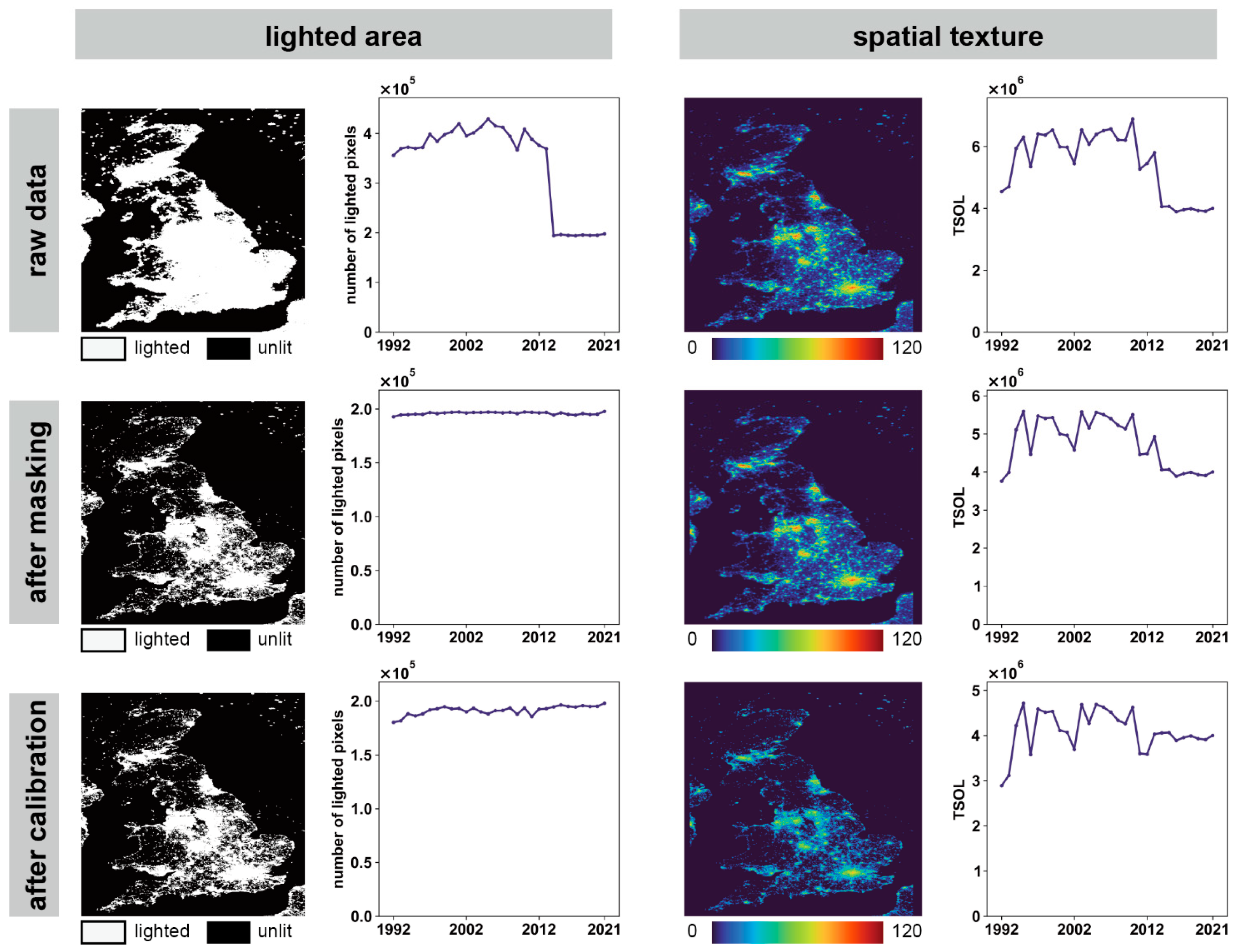
Masking and calibration are the key steps for spatial and temporal consistency. As shown in Figure 13, the case of the UK shows that masking reduces the spatial inconsistency of CCNL-DMSP with VNL-VIIRS, while calibration reduces the temporal inconsistency of CCNL-DMSP with the regressed VNL-VIIRS. Spatially, CCNL-DMSP has a larger spatial extent compared to VNL-VIIRS due to transit time and other sensor differences, and masking removes the different spatial extent, which accounts for 51.2% of the global lighted pixels of CCNL-DMSP. Without masking, the area of lighted pixels expands almost twice, which illustrates the necessity of masking. Temporally, the calibration avoids the misidentification of NTL time series development patterns. The Theil-Sen median trend analysis and Mann-Kendall trend test [44,45,46] are used to identify the time series of NTL, and the types are classified as significant increase, non-significant increase, significant decrease, and non-significant decrease. As shown in Table 3, unmasked and uncalibrated CCNL-DMSP has a large number of pixels with incorrect types compared to PCNL. The correct identification rates for significant increase, insignificant increase, significant decrease, and insignificant decrease are 84.4%, 20.3%, 54.2%, and 25.7%, respectively. The low correct identification rate for NTL types illustrates the need for calibration.
5.3. Limitations of PCNL
PCNL is a DMSP-like NTL dataset with a uniform spatial resolution compared to CCNL-DMSP. We discarded the advantage of the high resolution of VNL-VIIRS and resampled VNL-VIIRS to 30 arcsec, which was consistent with CCNL-DMSP. The reduction in spatial resolution is a loss of product quality; however, it is necessary to produce PCNL. The spatial resolution of VNL-VIIRS is higher than that of CCNL-DMSP, which means that four pixels of VNL-VIIRS correspond to one pixel of CCNL-DMSP. We can resample four pixels of VNL-VIIRS into one pixel by resampling, but it is not easy to do the opposite. Compared with the traditional regression method, machine learning and deep learning methods can compensate for this deficiency [25,47], which is worth exploring in the future.
All three NTL products have unreasonable fluctuations around 2005 due to the interannual inconsistency problem of DMSP-OLS, which is prominent during that time, and the interannual correction methods used for these products still fail to address the problem entirely. Among the interannual correction methods used by PCNL, ChenNTL, and LiNTL, the stepwise interannual correction method [17] used by LiNTL is the most effective. The method of the invariant region [36] used by CCNL-DMSP is relatively simple, but interannual fluctuations still need to be removed entirely. Some novel interannual consistency correction methods are proposed [48], which are worthy of continued exploration in the future.
6. Conclusions
In this study, we proposed the DMSP-OLS and NPP-VIIRS inter-correction methods. Based on the processed DMSP-OLS dataset CCNL-DMSP and the processed NPP-VIIRS dataset VNL-VIIRS, a set of long time series global NTL products PCNL (1992–2021), which meets pixel-scale research needs, was developed through the processes of outlier removal, resampling, masking, regression, and calibration. In order to examine the quality of PCNL, PCNL and two existing global long-time series NTL products, LiNTL and ChenNTL, are compared from several angles, including overall accuracy, spatial consistency, temporal consistency, and applicability in the socio-economic field.
PCNL demonstrates good overall accuracy at both the pixel-scale (R2: 0.93, RMSE: 0.77) and the city scale (R2: 0.98, RMSE: 1883.28). The spatial texture maps of PCNL show good spatial consistency in developing, developed, and war regions. At global and national scales, the plotted time series curves and calculated ANDI indicate a stable time trend and good temporal consistency for PCNL (ANDI: 0.023, global). In the bridging year of CCNL-DMSP and VNL-VIIRS (near 2013), PCNL well bridges CCNL-DMSP and VNL-VIIRS. At urban and pixel-scales, PCNL also performs well in stable developed regions, in stable developing regions, and regions experiencing sudden development and sudden disaster. At the global scale, PCNL has a high correlation coefficient with GDP (r: 0.945) and population (r: 0.971). For more than half of the countries, the correlation coefficients of PCNL with GDP and population are higher than the results of ChenNTL and LiNTL, which indicates the strong applicability of PCNL in the socio-economic domain.
Author Contributions
Conceptualization, X.C. (Xin Cao); Formal analysis, S.L.; Funding acquisition, X.C. (Xin Cao); Investigation, S.L. and L.L.; Methodology, S.L., X.C. (Xin Cao), C.Z. and N.J.; Supervision, X.C. (Xuehong Chen) and X.C. (Xihong Cui); Validation, S.L.; Writing—original draft, S.L. and X.C. (Xuehong Chen); Writing—review & editing, X.C. (Xin Cao) and X.C. (Xihong Cui). All authors have read and agreed to the published version of the manuscript.
Funding
This research was funded by the Special Project of Science and Technology Basic Resources Survey, Ministry of Science and Technology of China, grant number 2019FY202502.
Data Availability Statement
PCNL has been shared at https://zenodo.org/record/7612389 [35]. CCNL-DMSP can be obtained at https://doi.org/10.5281/zenodo.6644980. VNL-VIIRS can be obtained from https://eogdata.mines.edu/nighttime_light/annual/v21/. ChenNTL can be obtained from https://doi.org/10.7910/DVN/YGIVCD. LiNTL can be obtained from https://doi.org/10.6084/m9.figshare.9828827.v2. GDP and POP data can be obtained from https://data.worldbank.org/. National administrative division data can be obtained from https://www.resdc.cn/data.aspx?DATAID=205. Municipal administrative division data can be obtained from https://gadm.org/download_world.html. All of the above datasets were accessed on 7 July 2023. MATLAB codes developed and used in this study are available upon request from the corresponding author.
Conflicts of Interest
The authors declare no conflict of interest.
References
- Cao, X.; Chen, J.; Imura, H.; Higashi, O. A SVM-Based Method to Extract Urban Areas from DMSP-OLS and SPOT VGT Data. Remote Sens. Environ. 2009, 113, 2205–2209. [Google Scholar] [CrossRef]
- Zhang, Q.; Seto, K.C. Mapping Urbanization Dynamics at Regional and Global Scales Using Multi-Temporal DMSP/OLS Nighttime Light Data. Remote Sens. Environ. 2011, 115, 2320–2329. [Google Scholar] [CrossRef]
- Yang, Y.; Wu, J.; Wang, Y.; Huang, Q.; He, C. Quantifying Spatiotemporal Patterns of Shrinking Cities in Urbanizing China: A Novel Approach Based on Time-Series Nighttime Light Data. Cities 2021, 118, 103346. [Google Scholar] [CrossRef]
- Wang, Y.; Liu, Z.; He, C.; Xia, P.; Liu, Z.; Liu, H. Quantifying Urbanization Levels on the Tibetan Plateau with High-Resolution Nighttime Light Data. Geogr. Sustain. 2020, 1, 233–244. [Google Scholar] [CrossRef]
- Li, X.; Zhou, W. Dasymetric Mapping of Urban Population in China Based on Radiance Corrected DMSP-OLS Nighttime Light and Land Cover Data. Sci. Total Environ. 2018, 643, 1248–1256. [Google Scholar] [CrossRef] [PubMed]
- Tan, M.; Li, X.; Li, S.; Xin, L.; Wang, X.; Li, Q.; Li, W.; Li, Y.; Xiang, W. Modeling Population Density Based on Nighttime Light Images and Land Use Data in China. Appl. Geogr. 2018, 90, 239–247. [Google Scholar] [CrossRef]
- Wang, L.; Fan, H.; Wang, Y. Improving Population Mapping Using Luojia 1-01 Nighttime Light Image and Location-Based Social Media Data. Sci. Total Environ. 2020, 730, 139148. [Google Scholar] [CrossRef] [PubMed]
- Henderson, V.; Storeygard, A.; Weil, D.N. A Bright Idea for Measuring Economic Growth. Am. Econ. Rev. 2011, 101, 194–199. [Google Scholar] [CrossRef] [Green Version]
- Yu, B.; Shi, K.; Hu, Y.; Huang, C.; Chen, Z.; Wu, J. Poverty Evaluation Using NPP-VIIRS Nighttime Light Composite Data at the County Level in China. IEEE J. Sel. Top. Appl. Earth Obs. Remote Sens. 2015, 8, 1217–1229. [Google Scholar] [CrossRef]
- Min, B.; Gaba, K.M.; Sarr, O.F.; Agalassou, A. Detection of Rural Electrification in Africa Using DMSP-OLS Night Lights Imagery. Int. J. Remote Sens. 2013, 34, 8118–8141. [Google Scholar] [CrossRef]
- Cao, X.; Wang, J.; Chen, J.; Shi, F. Spatialization of Electricity Consumption of China Using Saturation-Corrected DMSP-OLS Data. Int. J. Appl. Earth Obs. Geoinf. 2014, 28, 193–200. [Google Scholar] [CrossRef]
- Wang, Y.; Wang, M.; Huang, B.; Li, S.; Lin, Y. Estimation and Analysis of the Nighttime PM2.5 Concentration Based on LJ1-01 Images: A Case Study in the Pearl River Delta Urban Agglomeration of China. Remote Sens. 2021, 13, 3405. [Google Scholar] [CrossRef]
- Elvidge, C.D.; Ghosh, T.; Hsu, F.-C.; Zhizhin, M.; Bazilian, M. The Dimming of Lights in China during the COVID-19 Pandemic. Remote Sens. 2020, 12, 2851. [Google Scholar] [CrossRef]
- Li, X.; Li, D. Can Night-Time Light Images Play a Role in Evaluating the Syrian Crisis? Int. J. Remote Sens. 2014, 35, 6648–6661. [Google Scholar] [CrossRef]
- Bennett, M.M.; Smith, L.C. Advances in Using Multitemporal Night-Time Lights Satellite Imagery to Detect, Estimate, and Monitor Socioeconomic Dynamics. Remote Sens. Environ. 2017, 192, 176–197. [Google Scholar] [CrossRef]
- Zhang, Q.; Pandey, B.; Seto, K.C. A Robust Method to Generate a Consistent Time Series From DMSP/OLS Nighttime Light Data. IEEE Trans. Geosci. Remote Sens. 2016, 54, 5821–5831. [Google Scholar] [CrossRef]
- Li, X.; Zhou, Y. A Stepwise Calibration of Global DMSP/OLS Stable Nighttime Light Data (1992–2013). Remote Sens. 2017, 9, 637. [Google Scholar] [CrossRef] [Green Version]
- Shen, Z.; Zhu, X.; Cao, X.; Chen, J. Measurement of Blooming Effect of DMSP-OLS Nighttime Light Data Based on NPP-VIIRS Data. Ann. GIS 2019, 25, 153–165. [Google Scholar] [CrossRef] [Green Version]
- Cao, X.; Hu, Y.; Zhu, X.; Shi, F.; Zhuo, L.; Chen, J. A Simple Self-Adjusting Model for Correcting the Blooming Effects in DMSP-OLS Nighttime Light Images. Remote Sens. Environ. 2019, 224, 401–411. [Google Scholar] [CrossRef]
- Wang, Z.; Román, M.; Kalb, V.; Shrestha, R.; Stokes, E.; Paynter, I. Uncertainties in VIIRS Nighttime Light Time Series Analysis. In Proceedings of the IGARSS 2020–2020 IEEE International Geoscience and Remote Sensing Symposium, Online, 26 September–2 October 2020; pp. 156–159. [Google Scholar]
- Elvidge, C.D.; Baugh, K.; Zhizhin, M.; Hsu, F.C.; Ghosh, T. VIIRS Night-Time Lights. Int. J. Remote Sens. 2017, 38, 5860–5879. [Google Scholar] [CrossRef] [Green Version]
- Zhou, Y.; Ma, T.; Zhou, C.; Xu, T. Nighttime Light Derived Assessment of Regional Inequality of Socioeconomic Development in China. Remote Sens. 2015, 7, 1242–1262. [Google Scholar] [CrossRef] [Green Version]
- You, H.; Yang, J.; Xue, B.; Xiao, X.; Xia, J.; Jin, C.; Li, X. Spatial Evolution of Population Change in Northeast China during 1992–2018. Sci. Total Environ. 2021, 776, 146023. [Google Scholar] [CrossRef]
- Zheng, Q.; Seto, K.C.; Zhou, Y.; You, S.; Weng, Q. Nighttime Light Remote Sensing for Urban Applications: Progress, Challenges, and Prospects. ISPRS J. Photogramm. Remote Sens. 2023, 202, 125–141. [Google Scholar] [CrossRef]
- Chen, Z.; Yu, B.; Yang, C.; Zhou, Y.; Yao, S.; Qian, X.; Wang, C.; Wu, B.; Wu, J. An Extended Time Series (2000–2018) of Global NPP-VIIRS-like Nighttime Light Data from a Cross-Sensor Calibration. Earth Syst. Sci. Data 2021, 13, 889–906. [Google Scholar] [CrossRef]
- Li, X.; Li, D.; Xu, H.; Wu, C. Intercalibration between DMSP/OLS and VIIRS Night-Time Light Images to Evaluate City Light Dynamics of Syria’s Major Human Settlement during Syrian Civil War. Int. J. Remote Sens. 2017, 38, 5934–5951. [Google Scholar] [CrossRef]
- Zhu, X.; Ma, M.; Yang, H.; Ge, W. Modeling the Spatiotemporal Dynamics of Gross Domestic Product in China Using Extended Temporal Coverage Nighttime Light Data. Remote Sens. 2017, 9, 626. [Google Scholar] [CrossRef] [Green Version]
- Hu, Y.; Zhang, Y. Global Nighttime Light Change from 1992 to 2017: Brighter and More Uniform. Sustainability 2020, 12, 4905. [Google Scholar] [CrossRef]
- Zhao, J.; Ji, G.; Yue, Y.; Lai, Z.; Chen, Y.; Yang, D.; Yang, X.; Wang, Z. Spatio-Temporal Dynamics of Urban Residential CO2 Emissions and Their Driving Forces in China Using the Integrated Two Nighttime Light Datasets. Appl. Energy 2019, 235, 612–624. [Google Scholar] [CrossRef]
- Chen, T.-H.K.; Prishchepov, A.V.; Fensholt, R.; Sabel, C.E. Detecting and Monitoring Long-Term Landslides in Urbanized Areas with Nighttime Light Data and Multi-Seasonal Landsat Imagery across Taiwan from 1998 to 2017. Remote Sens. Environ. 2019, 225, 317–327. [Google Scholar] [CrossRef]
- Zhao, M.; Zhou, Y.; Li, X.; Zhou, C.; Cheng, W.; Li, M.; Huang, K. Building a Series of Consistent Night-Time Light Data (1992–2018) in Southeast Asia by Integrating DMSP-OLS and NPP-VIIRS. IEEE Trans. Geosci. Remote Sens. 2020, 58, 1843–1856. [Google Scholar] [CrossRef]
- Zheng, Q.; Weng, Q.; Wang, K. Developing a New Cross-Sensor Calibration Model for DMSP-OLS and Suomi-NPP VIIRS Night-Light Imageries. ISPRS J. Photogramm. Remote Sens. 2019, 153, 36–47. [Google Scholar] [CrossRef]
- Li, X.; Zhou, Y.; Zhao, M.; Zhao, X. A Harmonized Global Nighttime Light Dataset 1992–2018. Sci Data 2020, 7, 168. [Google Scholar] [CrossRef]
- Zhao, C.; Cao, X.; Chen, X.; Cui, X. A Consistent and Corrected Nighttime Light Dataset (CCNL 1992–2013) from DMSP-OLS Data. Sci. Data 2022, 9, 424. [Google Scholar] [CrossRef] [PubMed]
- Li, S.; Cao, X. A Pixel-Scale Corrected Nighttime Light Dataset (PCNL, 1992–2021) Combining DMSP-OLS and NPP-VIIRS. Zenodo. 2023. Available online: https://doi.org/10.5281/zenodo.7612389 (accessed on 7 July 2023).
- Wu, J.; He, S.; Peng, J.; Li, W.; Zhong, X. Intercalibration of DMSP-OLS Night-Time Light Data by the Invariant Region Method. Int. J. Remote Sens. 2013, 34, 7356–7368. [Google Scholar] [CrossRef]
- Hu, Y.; Chen, J.; Cao, X.; Chen, X.; Cui, X.; Gan, L. Correcting the Saturation Effect in DMSP/OLS Stable Nighttime Light Products Based on Radiance-Calibrated Data. IEEE Trans. Geosci. Remote Sens. 2022, 60, 5602011. [Google Scholar] [CrossRef]
- Elvidge, C.D.; Zhizhin, M.; Ghosh, T.; Hsu, F.-C.; Taneja, J. Annual Time Series of Global VIIRS Nighttime Lights Derived from Monthly Averages: 2012 to 2019. Remote Sens. 2021, 13, 922. [Google Scholar] [CrossRef]
- Ma, T.; Zhou, C.; Pei, T.; Haynie, S.; Fan, J. Responses of Suomi-NPP VIIRS-Derived Nighttime Lights to Socioeconomic Activity in China’s Cities. Remote Sens. Lett. 2014, 5, 165–174. [Google Scholar] [CrossRef]
- Elvidge, C.D.; Baugh, K.; Ghosh, T.; Zhizhin, M.; Hsu, F.C.; Sparks, T.; Bazilian, M.; Sutton, P.C.; Houngbedji, K.; Goldblatt, R. Fifty Years of Nightly Global Low-Light Imaging Satellite Observations. Front. Remote Sens. 2022, 3, 919937. [Google Scholar] [CrossRef]
- Zheng, Z.; Yang, Z.; Chen, Y.; Wu, Z.; Marinello, F. The Interannual Calibration and Global Nighttime Light Fluctuation Assessment Based on Pixel-Level Linear Regression Analysis. Remote Sens. 2019, 11, 2185. [Google Scholar] [CrossRef] [Green Version]
- Elvidge, C.D.; Baugh, K.E.; Kihn, E.A.; Kroehl, H.W.; Davis, E.R.; Davis, C.W. Relation between Satellite Observed Visible-near Infrared Emissions, Population, Economic Activity and Electric Power Consumption. Int. J. Remote Sens. 1997, 18, 1373–1379. [Google Scholar] [CrossRef]
- Han, G.; Zhou, T.; Sun, Y.; Zhu, S. The Relationship between Night-Time Light and Socioeconomic Factors in China and India. PLoS ONE 2022, 17, e0262503. [Google Scholar] [CrossRef] [PubMed]
- Sen, P.K. Estimates of the Regression Coefficient Based on Kendall’s Tau. J. Am. Stat. Assoc. 1968, 63, 1379–1389. [Google Scholar] [CrossRef]
- Theil, H. A Rank-Invariant Method of Linear and Polynomial Regression Analysis. In Henri Theil’s Contributions to Economics and Econometrics: Econometric Theory and Methodology; Raj, B., Koerts, J., Eds.; Springer: Dordrecht, The Netherlands, 1992; pp. 345–381. ISBN 978-94-011-2546-8. [Google Scholar]
- Hamed, K.H.; Ramachandra Rao, A. A Modified Mann-Kendall Trend Test for Autocorrelated Data. J. Hydrol. 1998, 204, 182–196. [Google Scholar] [CrossRef]
- Sahoo, S.; Gupta, P.K.; Srivastav, S.K. Inter-Calibration of DMSP-OLS and SNPP-VIIRS-DNB Annual Nighttime Light Composites Using Machine Learning. GISci. Remote Sens. 2020, 57, 1144–1165. [Google Scholar] [CrossRef]
- Yang, L.; Cao, J.; Zhuo, L.; Shi, Q. A Novel Consistency Calibration Method for DMSP-OLS Nighttime Stable Light Time-Series Images. IEEE J. Sel. Top. Appl. Earth Obs. Remote Sens. 2022, 15, 2621–2631. [Google Scholar] [CrossRef]
Figure 1.
Flowchart of PCNL production.
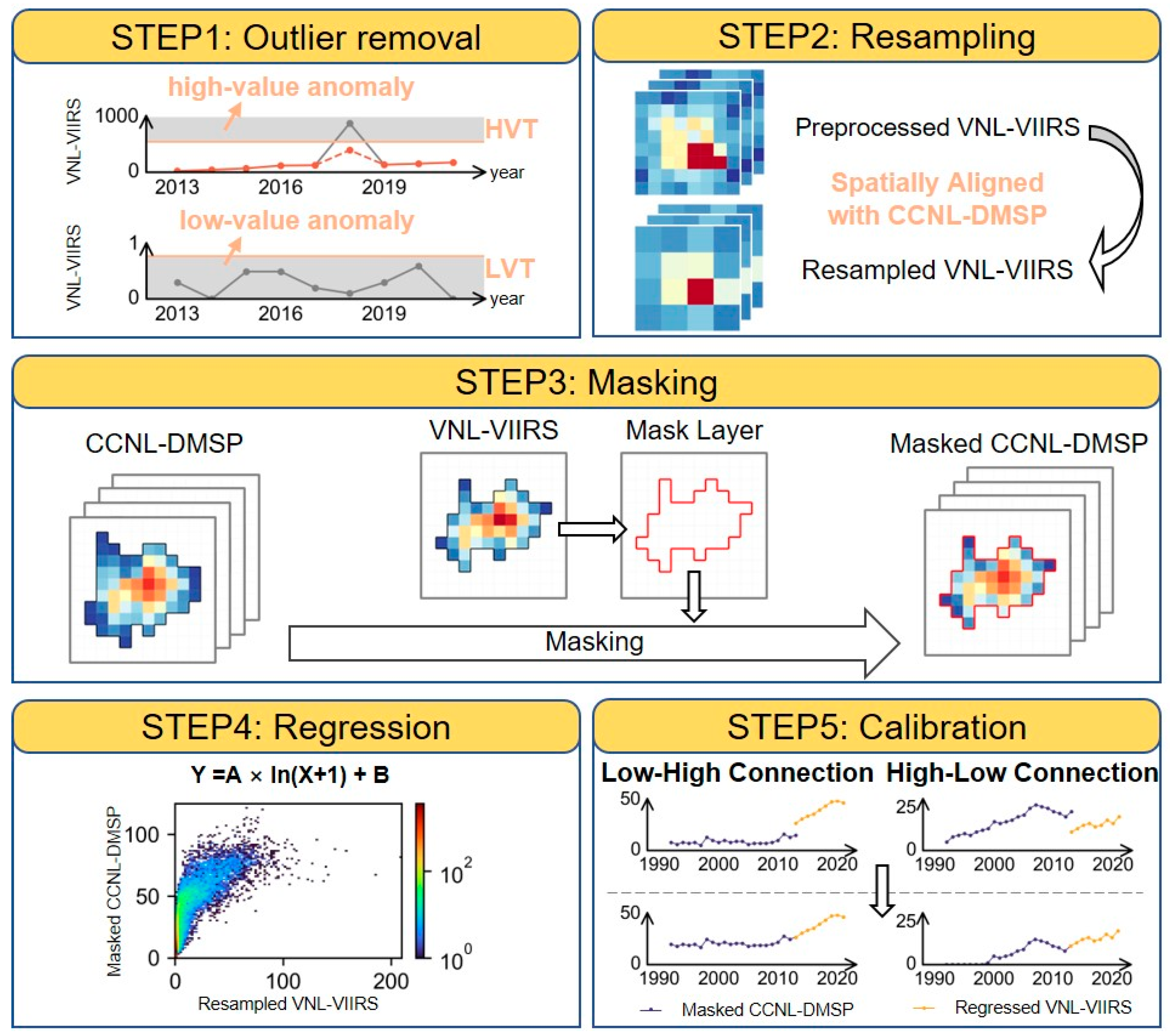
Figure 2.
Comparing the spatial extent differences between CCNL-DMSP and resampled VNL-VIIRS (unit: nWcm−2sr−1) in 2013.
Figure 2.
Comparing the spatial extent differences between CCNL-DMSP and resampled VNL-VIIRS (unit: nWcm−2sr−1) in 2013.
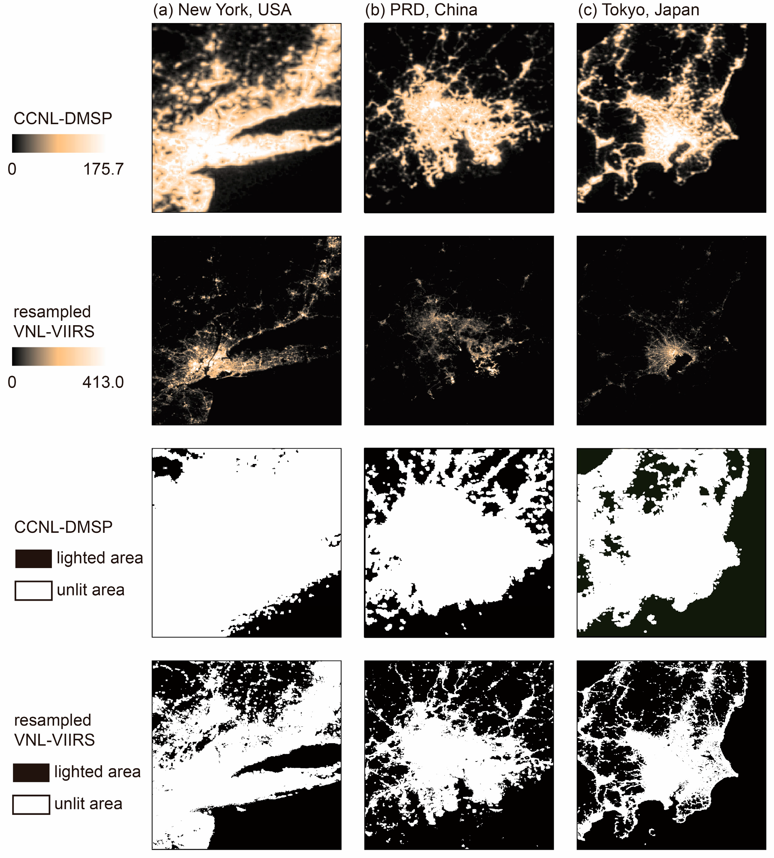
Figure 3.
Histogram of the corresponding resampled VNL-VIIRS (unit: nWcm−2sr−1) when DN values of masked CCNL-DMSP (DNCCNL-DMSP) in 2013 are in different intervals.
Figure 3.
Histogram of the corresponding resampled VNL-VIIRS (unit: nWcm−2sr−1) when DN values of masked CCNL-DMSP (DNCCNL-DMSP) in 2013 are in different intervals.

Figure 4.
Scattered density plots of masked CCNL-DMSP and resampled VNL-VIIRS (unit: nWcm−2sr−1) in 2013 in 6 cities: (a) Beijing, China; (b) Tokyo, Japan; (c) New Delhi, India; (d) Paris, France; (e) Berlin, Germany; and (f) London, UK. The color of the scatter represents the frequency.
Figure 4.
Scattered density plots of masked CCNL-DMSP and resampled VNL-VIIRS (unit: nWcm−2sr−1) in 2013 in 6 cities: (a) Beijing, China; (b) Tokyo, Japan; (c) New Delhi, India; (d) Paris, France; (e) Berlin, Germany; and (f) London, UK. The color of the scatter represents the frequency.
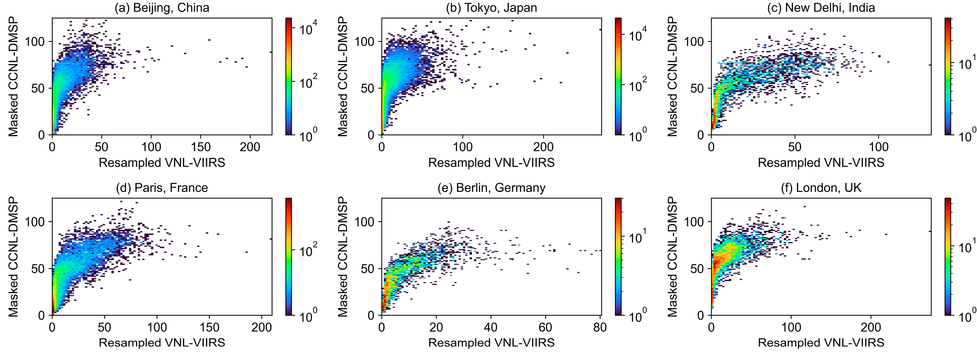
Figure 5.
Scatter density plots of resampled VNL-VIIRS and masked CCNL-DMSP. The dashed line is the regression model we chose.
Figure 5.
Scatter density plots of resampled VNL-VIIRS and masked CCNL-DMSP. The dashed line is the regression model we chose.

Figure 6.
Regression results for (a) the pixel-scale and (b) the city scale.
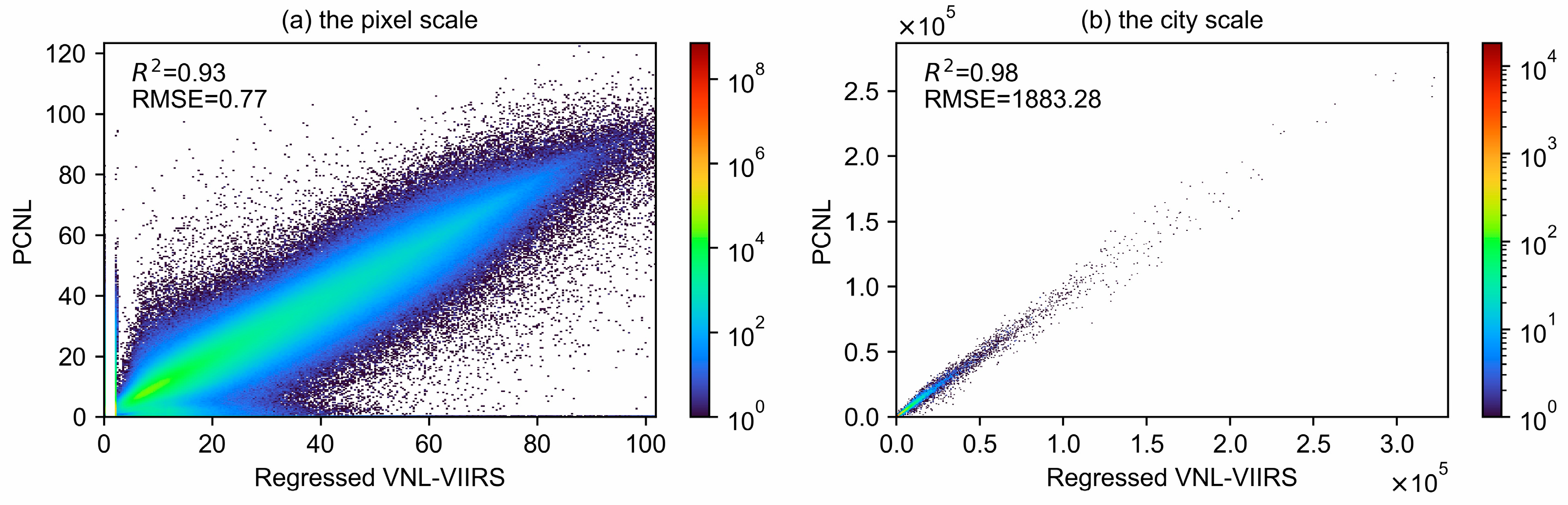
Figure 7.
Spatial texture maps comparing PCNL (1992–2021), LiNTL (1992–2018), and ChenNTL (2000–2020) in (a) BTH, China, (b) New York, US, and (c) Damascus, Syria. Due to the different distribution ranges of the values of the three NTL products and different areas of varying light values, to better demonstrate spatial details, develop color stretching rules based on the 99th percentile of each product in each area.
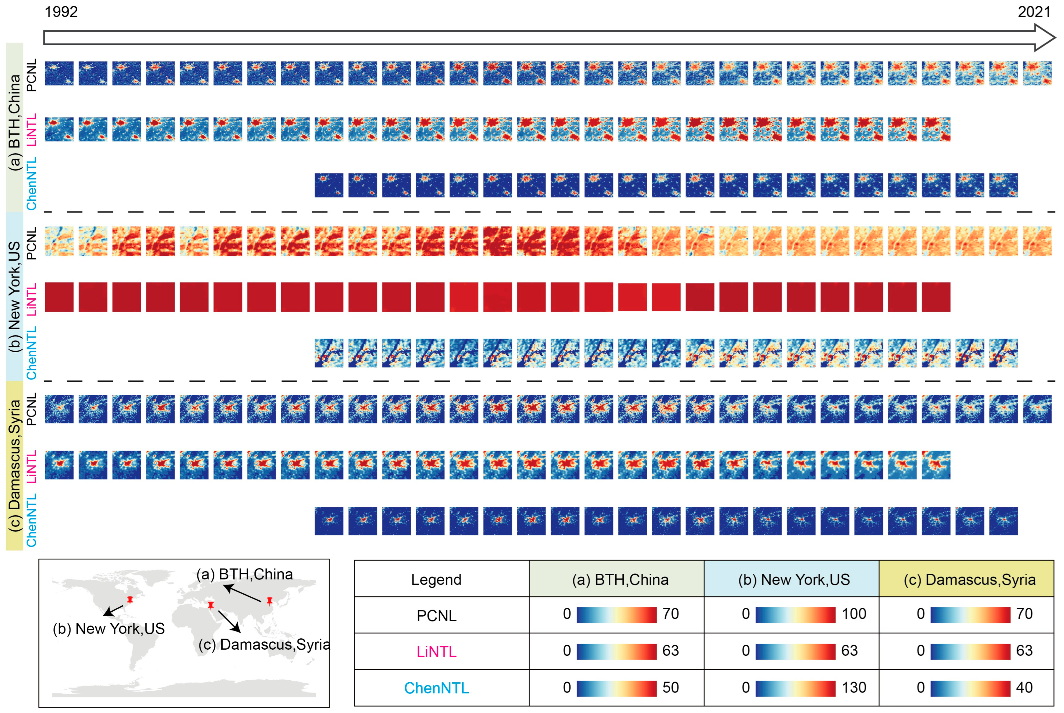
Figure 8.
DN curves comparing PCNL, LiNTL, and ChenNTL in BTH, China, in 2013. (a1–a3) are the spatial texture maps of three NTL products, and the four dashed lines in the maps correspond to the DN curves of (b1–b4).
Figure 8.
DN curves comparing PCNL, LiNTL, and ChenNTL in BTH, China, in 2013. (a1–a3) are the spatial texture maps of three NTL products, and the four dashed lines in the maps correspond to the DN curves of (b1–b4).
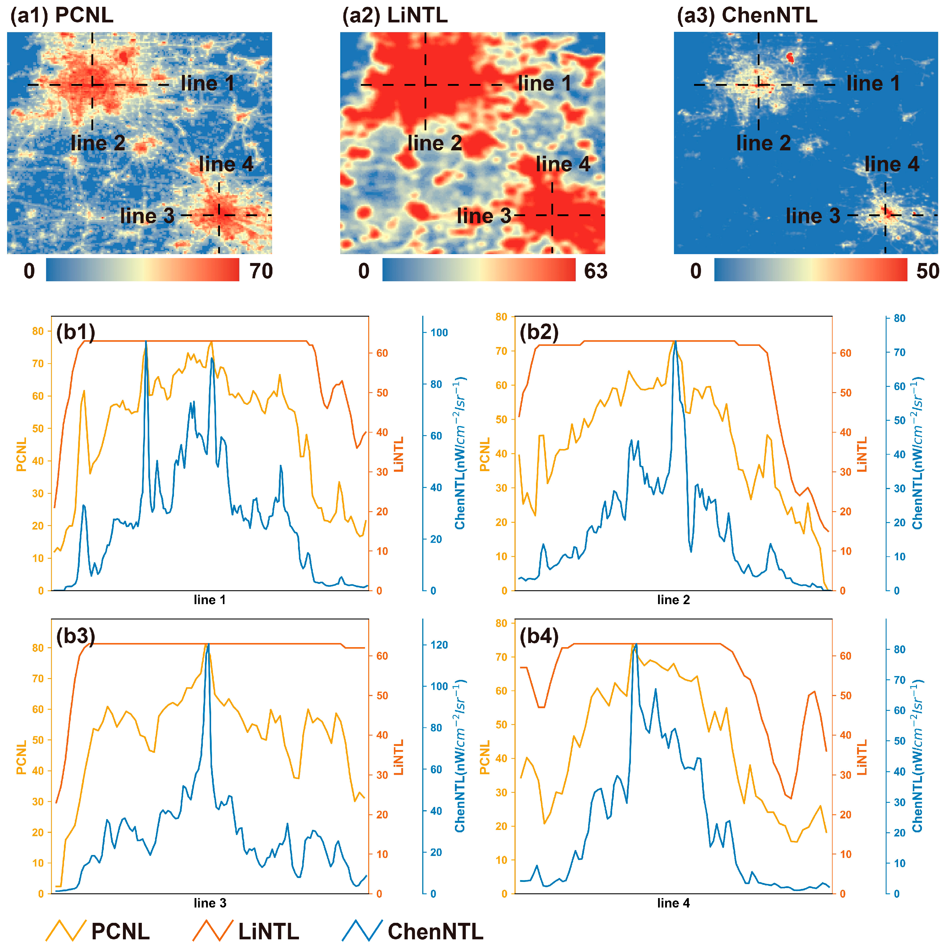
Figure 9.
Time series of the total sum of regional nighttime light comparing PCNL (1992–2021), LiNTL (1992–2018), and ChenNTL (2000–2020).
Figure 9.
Time series of the total sum of regional nighttime light comparing PCNL (1992–2021), LiNTL (1992–2018), and ChenNTL (2000–2020).
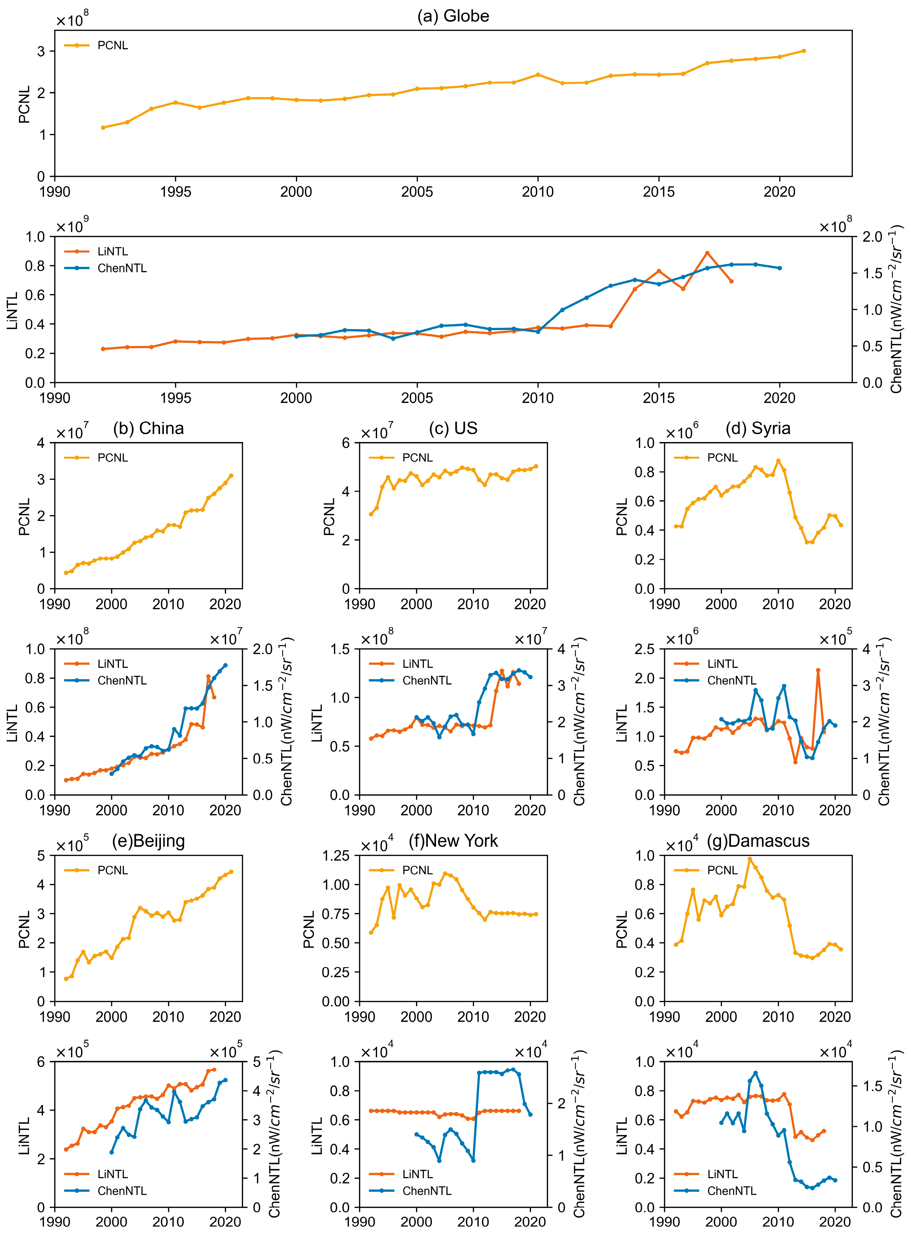
Figure 10.
ANDI comparing PCNL, LiNTL, and ChenNTL at the national scale.
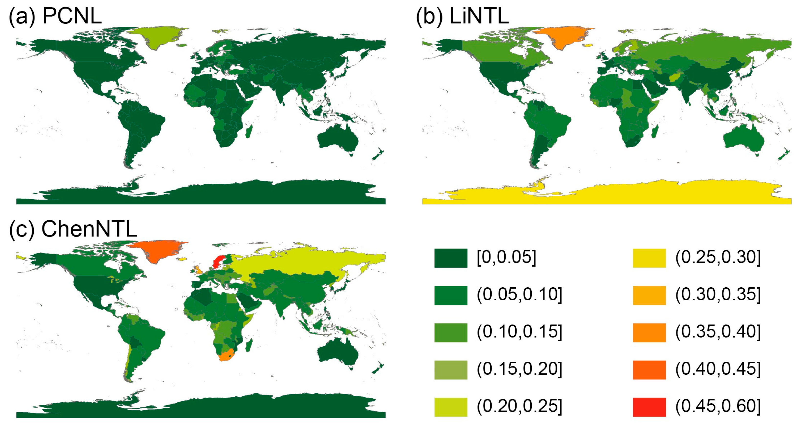
Figure 11.
Time series of pixel nighttime light comparing PCNL (1992–2021), LiNTL (1992–2018), and ChenNTL (2000–2020). For each case, the location on the world map is marked, and the PCNL nighttime light for band composite in the R (2021), G (2007), and B (1992) bands is shown. For each case, the time series of PCNL, LiNTL, and ChenNTL are plotted for the selected 9 pixels, marked as red or white dots. The administrative divisions were plotted on parts of the maps to aid point selection.
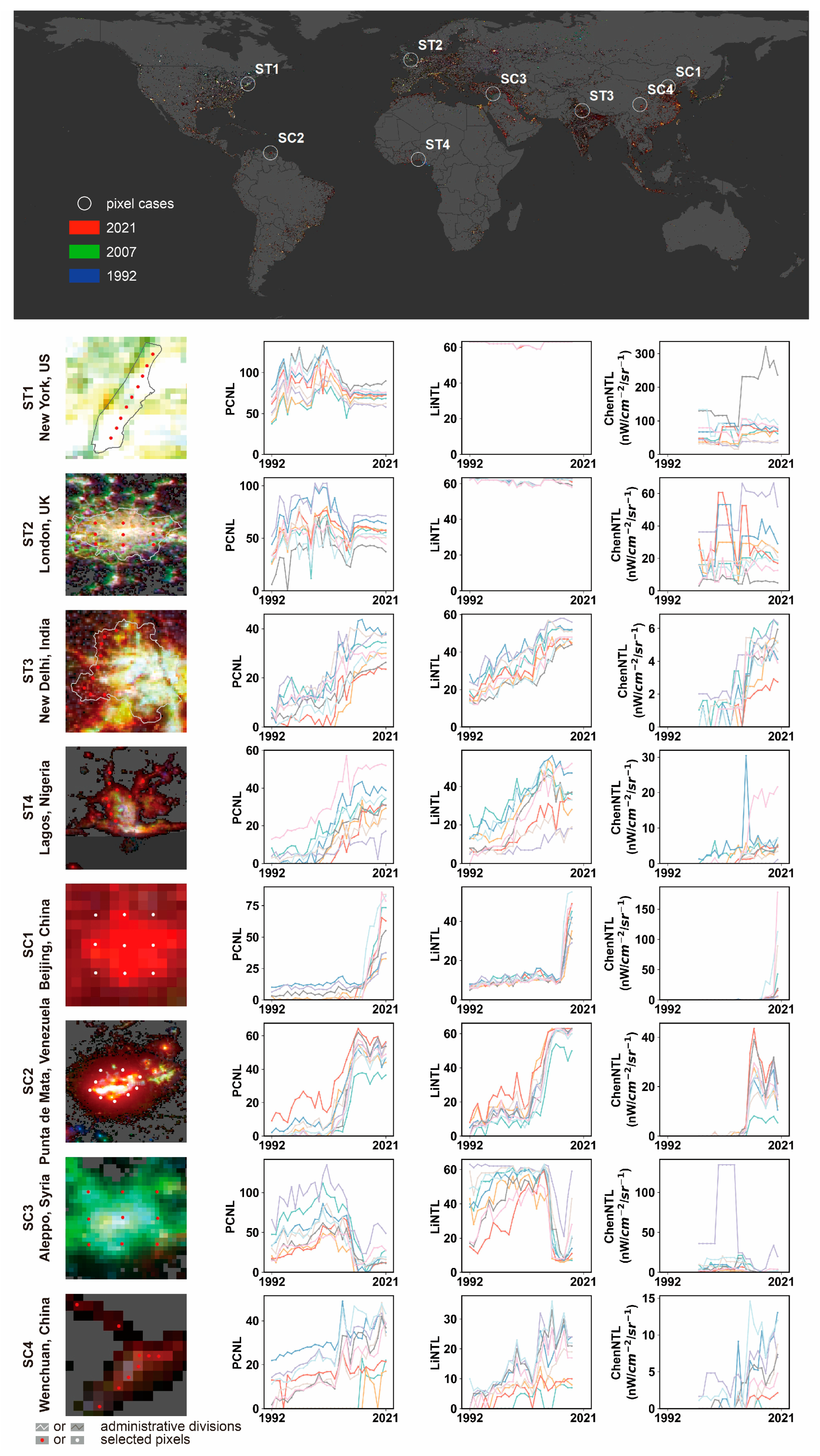
Figure 12.
Comparison of correlation coefficients between three types of NTL products (PCNL, LiNTL, and ChenNTL) and socio-economic data (GDP and POP) at the national scale. (a–c) are two-by-two comparisons of the correlation coefficients of the three NTL products and GDP. (d–f) are two-by-two comparisons of the correlation coefficients of the three NTL products and POP. For each point below the red dotted line, the NTL product represented by the horizontal coordinate of that point is superior to the NTL product represented by the vertical coordinate.
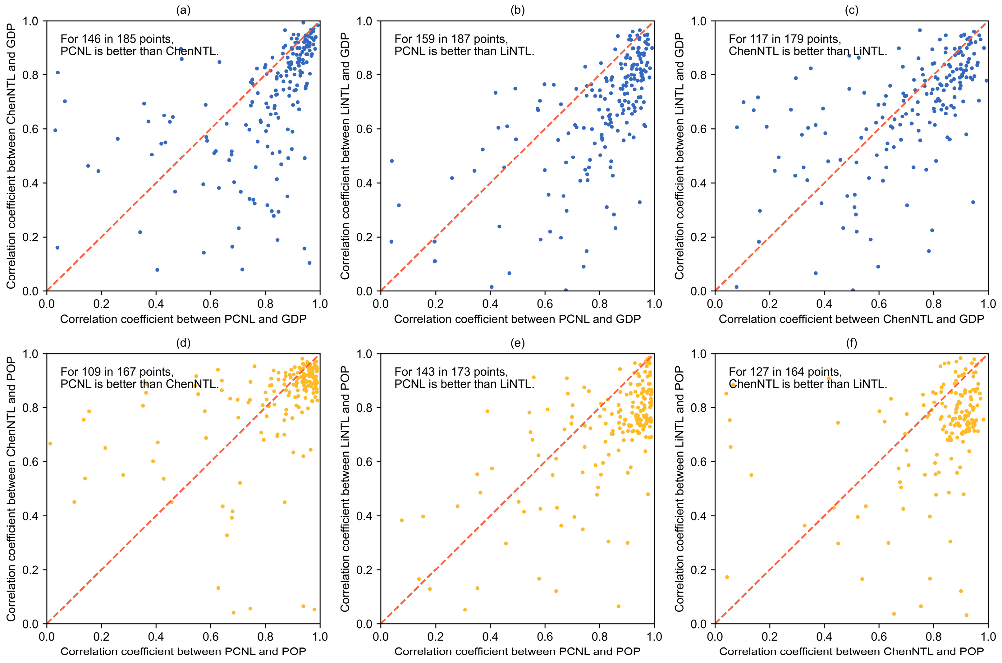
Figure 13.
Distribution of lighted area, number of lighted pixels, spatial texture, and TSOL comparing raw data, masked data, and calibrated data.
Figure 13.
Distribution of lighted area, number of lighted pixels, spatial texture, and TSOL comparing raw data, masked data, and calibrated data.

Table 1.
Summary of datasets used in this study.
| Role | Datasets | Time Range | Data Source |
|---|---|---|---|
| Production of PCNL | CCNL-DMSP | 1992–2013 | Zhao et al., 2022 [34] |
| VNL-VIIRS | April 2012–2021 | Earth Observation Group (https://eogdata.mines.edu/nighttime_light/annual/v21/) (accessed on 7 July 2023) | |
| Comparison with PCNL | ChenNTL | 2000–2020 | Chen et al., 2021 [25] |
| LiNTL | 1992–2018 | Li et al., 2020 [33] | |
| Examination of PCNL | GDP | 1992–2021 | World Bank (https://data.worldbank.org/indicator/NY.GDP.MKTP.CD) (accessed on 7 July 2023) |
| POP | 1992–2021 | World Bank (https://data.worldbank.org/indicator/SP.POP.TOTL) (accessed on 7 July 2023) | |
| Statistics and graphing | national administrative division data | Latest | Resource and Environment Science and Data Center (https://www.resdc.cn/data.aspx?DATAID=205) (accessed on 7 July 2023) |
| municipal administrative division data | Latest | Database of Global Administrative Areas (https://gadm.org/download_world.html) (accessed on 7 July 2023) |
Table 2.
Comparison summary of PCNL, LiNTL, and ChenNTL.
| Evaluation Perspectives | PCNL | LiNTL | ChenNTL |
|---|---|---|---|
| Time Horizon | 1992–2021 (updating) | 1992–2018 | 2000–2020 (updating) |
| Spatial Extent | Global | Global | Global |
| Spatial Resolution | 30 arc seconds (~1 km) | 30 arc seconds (~1 km) | 15 arc seconds (~500 m) |
| Overall Accuracy | Pixel-scale: R2 = 0.93, RMSE = 0.77 City scale: R2 = 0.98, RMSE = 1883.28 | Pixel-scale: R2 ≈ 0.5 in China | Pixel-scale: R2 = 0.87, RMSE = 2.96 nWcm−2sr−1 City scale: R2 = 0.95, RMSE = 3024.62 nWcm−2sr−1 |
| Spatial Consistency | Stable | Stable but saturated | Stable |
| Regional Temporal Consistency | Global: ANDI = 0.023 Developing regions: stable Developed regions: fluctuating then stable War regions: able to detect changes | Global: ANDI = 0.046 Developing regions: stable Developed region: saturated, with unreasonable abrupt changes War regions: able to detect changes | Global: ANDI = 0.042 Developing regions: stable Developed regions: fluctuating, with unreasonable abrupt changes War regions: able to detect changes |
| Pixel Temporal Consistency | Advantages: able to display stable trends and detect sudden changes Disadvantage: existence of interannual fluctuation, but acceptable | Advantages: able to display stable trends in low-value regions and detect sudden changes Disadvantage: disable to compare differences of values in high-value regions due to saturation | Advantages: able to display general trends and detect sudden changes Disadvantage: existence of many unreasonable abrupt changes and fluctuation over a larger range |
| Applicability in the socio-economic field | Global: r = 0.945 with GDP, r = 0.971 with POP Country scale: better than LiNTL and ChenNTL for both GDP and POP | Global: r = 0.776 with GDP, r = 0.815 with POP Country scale: worse than PCNL and ChenNTL for both GDP and POP | Global: r = 0.881 with GDP, r = 0.937 with POP Country scale: better than LiNTL, slightly worse than PCNL, for both GDP and POP |
Table 3.
Type identification of NTL time series curves before and after masking and calibration.
| Types Identified by PCNL | Types Identified by Unmasked and Uncalibrated CCNL-DMSP and Regressed VNL-VIIRS | |||
|---|---|---|---|---|
| Significant Increase | Non-Significant Increase | Significant Decrease | Non-Significant Decrease | |
| Significant increase | 84.4% | 8.1% | 0.9% | 6.6% |
| Non-significant increase | 48.7% | 20.3% | 11.8% | 19.2% |
| Significant decrease | 12.3% | 15.7% | 54.2% | 17.8% |
| Non-significant decrease | 28.4% | 17.9% | 28.1% | 25.7% |
Disclaimer/Publisher’s Note: The statements, opinions and data contained in all publications are solely those of the individual author(s) and contributor(s) and not of MDPI and/or the editor(s). MDPI and/or the editor(s) disclaim responsibility for any injury to people or property resulting from any ideas, methods, instructions or products referred to in the content. |
© 2023 by the authors. Licensee MDPI, Basel, Switzerland. This article is an open access article distributed under the terms and conditions of the Creative Commons Attribution (CC BY) license (https://creativecommons.org/licenses/by/4.0/).
Share and Cite
MDPI and ACS Style
Li, S.; Cao, X.; Zhao, C.; Jie, N.; Liu, L.; Chen, X.; Cui, X. Developing a Pixel-Scale Corrected Nighttime Light Dataset (PCNL, 1992–2021) Combining DMSP-OLS and NPP-VIIRS. Remote Sens. 2023, 15, 3925. https://doi.org/10.3390/rs15163925
AMA Style
Li S, Cao X, Zhao C, Jie N, Liu L, Chen X, Cui X. Developing a Pixel-Scale Corrected Nighttime Light Dataset (PCNL, 1992–2021) Combining DMSP-OLS and NPP-VIIRS. Remote Sensing. 2023; 15(16):3925. https://doi.org/10.3390/rs15163925
Chicago/Turabian StyleLi, Shijie, Xin Cao, Chenchen Zhao, Na Jie, Luling Liu, Xuehong Chen, and Xihong Cui. 2023. "Developing a Pixel-Scale Corrected Nighttime Light Dataset (PCNL, 1992–2021) Combining DMSP-OLS and NPP-VIIRS" Remote Sensing 15, no. 16: 3925. https://doi.org/10.3390/rs15163925
Note that from the first issue of 2016, this journal uses article numbers instead of page numbers. See further details here.