APO-ELM Model for Improving Azimuth Correction of Shipborne HFSWR

Abstract

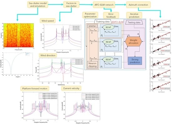
Shipborne high-frequency surface wave radar (HFSWR) has a wide range of applications and plays an important role in moving target detection and tracking. However, the complexity of the sea detection environment causes the target signals received by shipborne HFSWR to be seriously disturbed by sea clutter. Sea clutter increases the difficulty of azimuth estimation, resulting in a challenging problem for shipborne HFSWR. To solve this problem, a novel azimuth correction method based on adaptive boosting error feedback dynamic weighted particle swarm optimization extreme learning machine (APO-ELM) is proposed to improve the azimuth estimation accuracy of shipborne HFSWR. First, the sea clutter is modeled and simulated. Then, we study its characteristics and analyze the influence of its characteristics on the first-order clutter spectrum and target detection accuracy, respectively. In addition, the proposed improved particle swarm optimization (PSO) and adaptive neuron clipping algorithm are used to optimize the input parameters of the ELM network. Then, the network performs error feedback based on the optimized parameter performance and updates the feature matrix, which can give a minimum clutter-error estimation. After that, it iteratively trains multiple weak learners using the adaptive boosting (AdaBoost) algorithm to form a strong learner and make strong predictions. Finally, after error compensation, the best azimuth estimation results are obtained. The sample sets used for the APO-ELM network are obtained from field shipborne HFSWR data. The network training and testing features include the wind direction, sea current, wind speed, platform speed, and signal-to-clutter ratio (SCR). The experimental results show that this method has a lower root-mean-square error than the back-propagation neural network and support vector regression (SVR) azimuth correction methods, which verifies the effectiveness of the proposed method.

1. Introduction

High-frequency surface wave radar (HFSWR) operates in the high-frequency band (3–30 MHz) and is capable of the over-the-horizon detection of targets beyond the line of sight [1]. With its advantages of long observation distance, large coverage area, and all-weather operation, it plays an important role in vessel target monitoring and large-scale ocean exploration [2]. Shipborne HFSWR, as a new radar system, has more detection flexibility. However, due to the complex sea environment, serious clutter, interference, and noise are mixed into the target echoes. Sea clutter can especially lead to a severe decrease in SCR. The vessel target detection ability is greatly reduced due to an increase in detection errors and reduced accuracy of the target azimuth [3]. For HFSWR, azimuth estimation is of great importance for the accurate detection and tracking of vessel targets.

In the field of radar target detection and sea state remote sensing, the sea surface echo spectrum is the key research object. In target detection, sea surface echoes belong to the category of sea clutter, and it is crucial to suppress sea clutter to improve target detection. High-frequency electromagnetic waves interact with the ocean surface and produce sea surface echoes. Bragg resonance scattering occurs when the wavelength is half of the radar electromagnetic wave. This is referred to as “first-order sea clutter” and is the main source of interference for shipborne HFSWR. Sea clutter modeling methods can be divided into two categories: one based on a large number of clutter statistical models, and the other constructing first-order or second-order scattering cross-section equations based on the clutter-generation mechanism and simulating the sea surface echo spectrum [4,5,6,7]. Zhu et al. [8] conducted extensive theoretical studies of the effects of sea clutter on shore-based HFSWR. Walsh et al. [9,10] proposed first-order and second-order sea cross-section equations for HFSWR on floating ocean platforms, showing the effects of different sea conditions and platform motion under different sea states and frequencies. Sun et al. [11] derived first-order sea surface scattering equations for shipborne platforms under uniform motion and floating immobility to provide a theoretical basis.

In recent years, a great deal of research on the azimuth estimation and correction of shipborne HFSWR has been conducted. Traditional array direction-finding (DF), such as digital beamforming (DBF), is vulnerable to external factors, such as interference and noise, due to the limited array aperture and beamwidth. In addition, there are subspace-based algorithms represented by the multiple signal classification (MUSIC) algorithm, but the resolution and accuracy of multiple sources [12] is the main difficulty experienced when using the MUSIC algorithm. The long processing time and a large amount of spectral peak searching [13] can also lead to the degradation of the MUSIC algorithm’s accuracy. Wu et al. [14] used the ocean echo to calibrate the HFSWR phased array, transforming the channel calibration into parameter estimation and correcting the antenna gain and phase errors. Sun et al. [15] combined the oblique projection operator with the MUSIC algorithm to accurately distinguish between targets and interference under sea clutter spreading by exploiting the differences in echoes between target points and sea clutter in the space domain. Yang et al. [16] combined the internal factors of the platform to optimize the array steering vector and correct the azimuth error to achieve irregular array direction-of-arrival (DOA) estimation and correction. These algorithms are valid under uncertain circumstances but not applicable to complex marine environments without full consideration of sea clutter and interference.

Machine learning techniques have gradually gained popularity in target azimuth estimation due to their great robustness, powerful generalization ability, and adaptive ability. Like convolutional neural networks (CNN), support vector machine (SVM) [17,18,19,20] and back-propagation (BP) networks [21,22] are used to train samples and predict results. In [23], the target DF using CNN does not require a priori assumptions on array geometry but instead uses a multiclassification criterion to cascade the reconstructed spatial spectrum. However, the parameters affect the prediction and are limited to scenarios where the number of sources is smaller than the number of physical sensors. And, it cannot be used for underdetermined vectoring. Although SVM is slow to train, it can avoid falling into local optima [24,25]. BP networks can easily fall into local optima, resulting in decreased classification accuracy [21,22]. Unlike shore-based HFSWR, shipborne HFSWR remains in its infancy in the field of target azimuth estimation and correction research.

Based on the above, a new network structure for the vessel target azimuth correction problem is proposed in this paper. The extreme learning machine (ELM) is a neural network with a single hidden layer [26], which only needs to determine the number of neurons in the hidden layer and their activation function and randomly generate the input weights and the bias of that layer. This has the advantages of rapid learning and good generalizability. However, if the network model is constructed by simply initializing the parameters randomly, there are disadvantages, such as node redundancy and overload, reducing performance. Zhang et al. [27] used the particle swarm optimization (PSO) algorithm to optimize the parameters in the ELM network and improve azimuth estimation accuracy. However, this algorithm also has problems, such as poor local search ability and ease of falling into local extremes. In addition, the AdaBoost algorithm [28], originally proposed by Freund and Schapire in 1995 for classification problems, has the advantages of high prediction accuracy and ease of implementation. It was later extended to the field of regression with the emergence of the AdaBoost.R [29] algorithm. Zeng et al. [30] combined AdaBoost.R with ELM to obtain a regression model, which achieved a better result.

In this paper, a target azimuth correction method based on an adaptive boosting error feedback dynamic weighted particle swarm optimization extreme learning machine (APO-ELM) is proposed to solve the problem of low target azimuth estimation accuracy. In this paper, based on a sea clutter modeling simulation, we first obtain the main factors affecting sea clutter (e.g., wind direction, wind speed, platform forward motion, and current velocity) and show that sea clutter affects the target DF. Then, we discuss the influence of wind direction, current, wind speed, and platform forward motion of the clutter characteristics on the first-order clutter spectrum and target azimuth estimation accuracy, which serves as the basis for correcting the azimuth estimation under the influence of sea clutter. Then, we optimize the ELM network model using the improved PSO and neuron cropping. The error feedback (EF) is performed on the output layer to obtain the best parameters. After that, we use the AdaBoost algorithm to predict this model iteratively and ultimately achieve accurate azimuth correction. This paper is organized as follows. Section 2 briefly introduces sea clutter modeling and simulation. Section 3 analyzes the influence of clutter characteristics on the first-order echo spectrum and directional accuracy. In Section 4, an azimuth correction method based on APO-ELM is proposed to correct the DF error caused by clutter. In Section 5, the experimental evaluation results are provided using the new method and compared with other machine learning methods to verify its effectiveness. Finally, Section 6 presents the conclusions.

2. Sea Clutter Spectrum Model and Simulation

The interaction of high-frequency electromagnetic waves with the ocean surface generates sea surface echoes (that is, sea clutter). The study of the sea clutter spectral characteristics is important for clutter modeling and suppression. Since the energy of the motion-induced peak in the second-order spectrum is smaller than that of the first-order spectrum, we focus on the factors related to the DOA accuracy in the first-order echo spectrum. This section is divided into two subsections to model and simulate the echo signal: Section 2.1 constructs the first-order scattering cross-section equations to establish the time domain model of the sea surface echo signal; Section 2.2 simulates the sea surface echo spectrum.

2.1. Received Signal Model

The condition for producing Bragg resonant scattering via high-frequency electromagnetic waves interacting with the sea surface is

$$\mathrm{L}\cos \mathrm{\Delta }=\lambda /2,$$

(1)

where $\mathrm{L}$ is the wavelength, $\lambda$ is the electromagnetic wavelength, and $\mathrm{\Delta }$ is the grazing angle.

The wave velocity satisfying the first-order Bragg scattering condition is

$$v_{\mathrm{B}}=\sqrt{\frac{gL}{2\pi }}=\frac{1}{2}\sqrt{\frac{g\lambda }{\pi }}$$

(2)

Therefore, the first-order sea clutter Doppler frequency of a shore-based single-station HFSWR can be expressed as

$$f_{\mathrm{d}}=\pm f_{\mathrm{B}}=\pm \frac{2v_{\mathrm{B}}}{\lambda }=\pm \frac{2\sqrt{\raisebox{1ex}{$g\lambda $}\!\left/ \!\raisebox{-1ex}{$4\pi $}\right.}}{\lambda }=\pm \sqrt{\frac{g}{\pi \lambda }}=\pm 0.102\sqrt{f_0},$$

(3)

where $g$ is the gravitational acceleration, $f_0$ is the operating frequency of the shore-based HFSWR, and $\pm$ indicates the heading (toward or away from the radar station) caused by the ocean current. From Equation (3), it is evident that the first-order echo Doppler frequency is only related to the radar operating frequency and is independent of the incident azimuth of the sea surface micro-element.

For shipborne HFSWR, when the platform is in uniform linear motion, the first-order sea clutter Doppler frequency is

$$f_{\mathrm{d}}=\pm f_{\mathrm{B}}+f_{\mathrm{v}}({\theta }_s)+f_{\mathrm{c}}({\theta }_s)$$

(4)

$$f_{\mathrm{v}}({\theta }_s)=\frac{2v_{\mathrm{p}}\sin {\theta }_s}{\lambda },$$

(5)

$$f_{\mathrm{c}}({\theta }_s)=\frac{2v_{\mathrm{c}}\sin {\theta }_s}{\lambda },$$

(6)

where ${\theta }_s$ is the angle between the clutter and the forward direction of the platform (which is the direction of the Bragg scattering wave propagation), with the normal array as 0° and clockwise as positive, where $v_{\mathrm{p}}$ is the platform speed, $v_{\mathrm{c}}$ is the current speed, $f_{\mathrm{v}}$ is the radial Doppler effect caused by the platform forward motion, and $f_{\mathrm{c}}$ is the radial Doppler effect caused by the current.

As previously mentioned, the first-order Doppler frequency of the shore-based HFSWR is only related to the radar operating frequency in the ideal case without considering the surface current field. As shown in Figure 1a, the space-frequency lines of the shore-based HFSWR first-order sea surface echo Doppler spectrum are two straight lines symmetrical around the zero frequency. Therefore, the Doppler frequencies of the sea surface echo signals of different incident azimuths are $\pm f_B$. However, according to Equation (4), Figure 1b shows that the shipborne HFSWR first-order sea surface echo Doppler frequency caused by the Doppler frequency shift due to platform forward motion and current is no longer constant and instead has a linear relationship with the sine function of the azimuth. This is due to the radial velocity components generated on the microelements in different directions within the beam scanning range, which also makes the first-order sea clutter waves coupled in the space and Doppler domains.

The first-order radar cross-section (RCS) of sea clutter in a time domain can be simplified as

$${\sigma }_{\mathrm{s}}(R_r,{\theta }_s,t)=A_{+}{e}^{\mathrm{j}2\pi (f_{\mathrm{B}}+f_{\mathrm{v}}({\theta }_s)+f_{\mathrm{c}}({\theta }_s))t}+A_{-}{e}^{\mathrm{j}2\pi (-f_{\mathrm{B}}+f_{\mathrm{v}}({\theta }_s)+f_{\mathrm{c}}({\theta }_s))t}$$

(7)

where $\mathrm{j}$ is the imaginary unit and $A_{\pm }$ is the sea surface scattering unit echo signal amplitude, which is a zero-mean complex Gaussian random variable with a variance proportional to the energy of the wave spectrum. $A_{\pm }$ reflects the variation in echo signal amplitude due to the randomness of the ocean surface and the anisotropy of the mean wind and wave heights.

The directional wave spectrum $S(k,\theta )$ is the main factor affecting the first-order sea clutter spectrum, which is used to describe the heave height of the sea surface and can be described by a Gaussian distribution to delineate its stochastic properties. For a fully developed sea surface, the wave height spectrum size can be described by the undirected energy spectrum $S(k)$ and a factor $G(\theta )$ characterizing the directionality, where ${\displaystyle {\int }_{-\pi }^{\pi }G(\theta )}=1$. The expression of the wave height spectrum is as follows:

$$S(k,\theta )=S(k)G(\theta )$$

(8)

where $k$ is the wave vector and $\theta$ is the angle between the electromagnetic wave and the sea wave.

In this paper, the undirected energy spectrum is used to describe the wave amplitude distribution at different frequencies using the Pierson–Moskowitz (P-M) wave spectrum [31,32].

The undirected wave spectrum of the P-M spectrum is as follows:

$$S(k)=\frac{1}{2}\left[\frac{0.0045}{k^3}{e}^{-0.74{(\frac{k_c}{k})}^2}\right]$$

(9)

$$k_c=\frac{g}{U_{10}^2}$$

(10)

where $k_c$ represents the cutoff beam, which describes the effect of wind speed $U_{10}$ on the wave spectrum.

In contrast, in the P-M spectrum, the effect of the sea surface wind direction is reflected in the direction factor $G(\theta )$ that can be reduced to the following form:

$$G(\theta )=\frac{4}{3\pi }{\cos }^{\mathrm{s}}(\frac{\theta -{\theta }_w}{2})$$

(11)

where $\mathrm{s}$ is the expansion factor used to describe the degree of expansion of the waves to the wave height spectrum when the sea surface wind direction changes.

By substituting Equations (9) and (11) into Equation (8), we obtain the expressions for the sea surface wind speed and wind direction:

$$S(k_{\mathrm{w}},{\theta }_s)=\frac{1}{2}[\frac{0.0045}{k_{\mathrm{w}}^3}{e}^{\frac{-0.74g^2}{k_{\mathrm{w}}^3{U}_{10}^4}}][\frac{4}{3\pi }{\cos }^{\mathrm{s}}(\frac{{\theta }_s-{\theta }_{\mathrm{w}}}{2})]$$

(12)

Under fully developed sea conditions, the relevant parameters are as follows:

$$\begin{array}{l}{A}_{\pm }=a_{\pm }+i{b}_{\pm }\\ \left|a_{\pm }\right|=\left|b_{\pm }\right|=0\\ \left|a_{\pm }^2\right|=\left|b_{\pm }^2\right|=\eta \\ \eta ={\cos }^{\mathrm{s}}\left(\frac{{\theta }_s-{\theta }_{\mathrm{w}}}{2}\right)+\epsilon \end{array}$$

(13)

where $\epsilon =0.01$, $\mathrm{s}=4$, ${\theta }_{\mathrm{w}}$ is the angle between the radar beam direction and the wind direction on the sea surface, and $U_{10}$ is the wind speed 10 m above the sea surface.

From the above analysis, it can be concluded that the wave spectrum is influenced by the sea surface wind speed and wind direction. The first-order sea clutter spectrum of shore-based HFSWR has two symmetrical peaks. For shipborne HFSWR, the first-order sea clutter spectrum will be broadened to a certain extent. According to Equation (4), it is related to the operating frequency, incident direction, and velocity of the shipborne HFSWR.

We consider a wide-beam HFSWR system using linear frequency modulated intermittent continuous waves (LFMICW). As shown in Figure 2, the transmitting array elements are located in the center of the ship, and the receiving array elements are uniformly located on the right side of the ship. Under the uniform linear motion of the shipborne platform, the sea surface is divided into several sea surface microelements, with the forward direction of the platform as the X-axis and the normal direction of the forward direction as the Y-axis. The echo signal of the same distance unit is regarded as a circular echo of the sea surface in each azimuth. In Figure 2, $R$ represents the distance between the shipborne motion platform and the target, and ${\theta }_s$ represents the azimuth of the divided different sea surface scattering microelement with respect to the shipborne platform, with the normal array as 0° and clockwise as positive. The angular resolution $\mathrm{\Delta }\theta$ is set to 0.1°, and the distance resolution is obtained from the ratio of the speed of light to the radar bandwidth (i.e., $\mathrm{\Delta }R=c/2B$), where $R=r\mathrm{\Delta }R, 1\le r\le D_{\max }$, $D_{\max }$ is the total number of distance units. Both of them are combined to be jointly located at the $(r,s)\mathrm{th}$ sea surface micro-element observation region.

By considering the background noise and adding the vessel target, the sea clutter simulation signal can be expressed as

$$x(R_r,{\theta }_s,t)={\displaystyle \sum _{r,s}\kappa (r)\gamma ({\theta }_s)\alpha ({\theta }_s)}{\sigma }_{\mathrm{s}}(R_r,{\theta }_s,t)+\alpha (\theta ){\sigma }_{\mathrm{T}}(t)+e(t),$$

(14)

where $R_r$ is the r-distance unit, ${\theta }_s$ is the s-angle unit, $\theta$ is the target azimuth angle, and $\gamma ({\theta }_s)$ is the array antenna error vector. In the ideal case of representing the s-angle element, the default error of each element antenna is 1. $\alpha ({\theta }_s)$ is the array steering vector. In this paper, a linear inhomogeneous array with N array elements is used, the direction of the X-axis is the inverse direction of the forward motion of the platform, and the direction of the Y-axis is the normal direction of the HFSWR array. We chose the antenna located at the origin as the reference array element, set the coordinates of the array element as $(x_k,y_k)$, (i.e., the horizontal and vertical coordinates of the array element $k$), set the amplitude $a(t)$ as 1 by default, and established that $p({\theta }_s)$ is the overall phase change of the antenna array. The angular resolution is $\mathrm{\Delta }\theta$. The angle range is $(-{\theta }_k,{\theta }_k)$, ${\theta }_s\in (-{\theta }_k,{\theta }_k)$ and there are M angle intervals. That is,

$$\alpha ({\theta }_s)={\left[\begin{array}{cccc}{e}^{j2\pi \frac{x_1\sin {\theta }_s+y_1\cos {\theta }_s}{\lambda }}& e^{j2\pi \frac{x_2\sin {\theta }_s+y_2\cos {\theta }_s}{\lambda }}& \cdots & e^{j2\pi \frac{x_N\sin {\theta }_s+y_N\cos {\theta }_s}{\lambda }}\end{array}\right]}^{\mathrm{T}}$$

(15)

which gives

$$\begin{array}{c}{\displaystyle \sum _{{\theta }_s=-{\theta }_k}^{{\theta }_k}\alpha ({\theta }_s)}={\displaystyle \sum _{{\theta }_s=-{\theta }_k}^{{\theta }_k}a(t)p({\theta }_s)}\hfill \\ \hfill \hspace{1em}\hspace{1em}\hspace{1em}\hspace{1em} =\left[\begin{array}{c}{\displaystyle \sum _{m=1}^M\cos 2\pi \frac{x_1\sin (-{\theta }_k+(m-1)\mathrm{\Delta }\theta )+y_1\cos (-{\theta }_k+(m-1)\mathrm{\Delta }\theta )}{\lambda }}\\ {\displaystyle \sum _{m=1}^M\cos 2\pi \frac{x_2\sin (-{\theta }_k+(m-1)\mathrm{\Delta }\theta )+y_2\cos (-{\theta }_k+(m-1)\mathrm{\Delta }\theta )}{\lambda }}\\ \cdots \\ {\displaystyle \sum _{m=1}^M\cos 2\pi \frac{x_N\sin (-{\theta }_k+(m-1)\mathrm{\Delta }\theta )+y_N\cos (-{\theta }_k+(m-1)\mathrm{\Delta }\theta )}{\lambda }}\end{array}\right]\end{array}$$

(16)

Let

$$\varphi (m,n,t)={\displaystyle \sum _{m=1}^M\left(\cos (2\pi f_{\mathrm{v}}(-{\theta }_k+(m-1)\mathrm{\Delta }\theta )t+2\pi \frac{x_n\sin (-{\theta }_k+(m-1)\mathrm{\Delta }\theta )+y_n\cos (-{\theta }_k+(m-1)\mathrm{\Delta }\theta )}{\lambda }\right)}$$

We can then obtain a target-free sea clutter echo signal:

$$\begin{array}{c}{x}_s(t)={\displaystyle \sum _{r,s}\kappa (r)\gamma ({\theta }_s){\sigma }_{\mathrm{S}}(t)p({\theta }_S)}\hfill \\ \hspace{1em}\hspace{1em}={\displaystyle \sum _{s}A\cos 2\pi f_{\mathrm{B}}t{e}^{\mathrm{j}2\pi f_{\mathrm{v}}({\theta }_s)t}p({\theta }_s)}\hfill \\ \hspace{1em}\hspace{1em}=\left[\begin{array}{c}A\cos 2\pi f_{\mathrm{B}}t({\displaystyle \sum _{m=1}^M\cos (2\pi f_{\mathrm{v}}(-{\theta }_k+(m-1)\mathrm{\Delta }\theta )t+2\pi \frac{x_1\sin (-{\theta }_k+(m-1)\mathrm{\Delta }\theta )+y_1\cos (-{\theta }_k+(m-1)\mathrm{\Delta }\theta )}{\lambda }})\\ A\cos 2\pi f_{\mathrm{B}}t({\displaystyle \sum _{m=1}^M\cos (2\pi f_{\mathrm{v}}(-{\theta }_k+(m-1)\mathrm{\Delta }\theta )t+2\pi \frac{x_2\sin (-{\theta }_k+(m-1)\mathrm{\Delta }\theta )+y_2\cos (-{\theta }_k+(m-1)\mathrm{\Delta }\theta )}{\lambda }})\\ ⋮\\ A\cos 2\pi f_{\mathrm{B}}t({\displaystyle \sum _{m=1}^M\cos (2\pi f_{\mathrm{v}}(-{\theta }_k+(m-1)\mathrm{\Delta }\theta )t+2\pi \frac{x_N\sin (-{\theta }_k+(m-1)\mathrm{\Delta }\theta )+y_N\cos (-{\theta }_k+(m-1)\mathrm{\Delta }\theta )}{\lambda }})\end{array}\right]\hfill \\ \hspace{1em}\hspace{1em}=A\cos 2\pi f_{\mathrm{B}}t{\left[\begin{array}{cccc}\varphi (m,1,t)& \varphi (m,2,t)& \cdots & \varphi (m,N,t)\end{array}\right]}^{\mathrm{T}}\hfill \end{array}$$

(17)

Here, $\kappa (r)$ indicates the decay function, specifically,

$$\kappa (r)=\frac{P_{\mathrm{t}}{G}_{\mathrm{t}}{G}_{\mathrm{r}}{\lambda }^2|F(r){|}^4}{{(4\pi )}^3{r}^4},$$

(18)

where $P_{\mathrm{t}}$ denotes the radar transmitting power, $G_{\mathrm{t}}$ and $G_{\mathrm{r}}$ denote the antenna directionality coefficient between the receiver and the transmitter, $\lambda$ is the radar wavelength, $r$ is the distance of the scattering unit on a given sea surface, and $F(r)$ denotes the ground-wave attenuation function:

Since the sea surface in a real situation is undulating and rough, the surface impedance attenuation function model of the rough surface [33] is used in this paper. Specifically,

$$F(r)=1-\mathrm{j}\sqrt{\pi \rho }{e}^{-\rho }\mathrm{erfc}(\mathrm{j}\sqrt{\rho }),$$

(19)

$$\rho =-\frac{\mathrm{j}\pi {\tau }^2{r}^{2.5}}{\lambda },$$

(20)

$$\tau =\frac{\sqrt{({\epsilon }_{\mathrm{r}}-\mathrm{j}60\sigma \lambda -1)}}{{\epsilon }_{\mathrm{r}}-\mathrm{j}60\sigma \lambda },$$

(21)

where $\tau$ is the rough surface impedance, ${\epsilon }_{\mathrm{r}}$ is the dielectric constant, $\sigma$ is the seawater conductivity, and $\mathrm{erfc}(·)$ is the complementary error function.

${\sigma }_{\mathrm{T}}(t)$ is the complex envelope form of the target reflection signal, expressed as

$${\sigma }_{\mathrm{T}}(t)=u(t)e^{\mathrm{j}2\pi f_{\mathrm{T}}t},$$

(22)

with

$$f_{\mathrm{T}}=\frac{2(v_{\mathrm{T}}\sin {\theta }_{\mathrm{T}}+v_{\mathrm{p}}\sin {\theta }_{\mathrm{T}})}{\lambda },$$

(23)

where $u(t)$ is the complex envelope of the target signal, $f_{\mathrm{T}}$ is the target’s Doppler frequency, ${\theta }_{\mathrm{T}}$ is the target azimuth, $v_{\mathrm{T}}$ is the target speed value, and $v_{\mathrm{p}}$ is the platform speed value.

Eventually, the target reflection signal is obtained, that is,

$$\begin{array}{l}{x}_{\mathrm{T}}(t)=\alpha (\theta ){\sigma }_{\mathrm{T}}(t)+n(t)\\ ={\left[\begin{array}{cccc}{e}^{j2\pi \frac{x_1\sin \theta +y_1\cos \theta }{\lambda }}& e^{j2\pi \frac{x_2\sin \theta +y_2\cos \theta }{\lambda }}& \cdots & e^{j2\pi \frac{x_N\sin \theta +y_N\cos \theta }{\lambda }}\end{array}\right]}^{\mathrm{T}}{\sigma }_T(t)+n(t)\end{array}$$

(24)

2.2. Simulation and Analysis of the Model

We simulated the received echo signal model to investigate the effect of sea clutter on the Doppler spectrum and target DF.

The simulation process was as follows:

• Set the radar system parameters and shipborne platform-related parameters to solve for the distance resolution.
• Generate the $f_d$ time domain sequence of a certain azimuth following Equation (4).
• Using Equation (9), multiply the array steering vector and antenna error vector to obtain the clutter time domain sequence.
• Add distance information to the clutter time domain sequence and multiply the distance attenuation function at different distance units.
• Add the target information. Set the parameters of target distance, velocity, and azimuth, and add the target information to the corresponding distance units.
• Repeat steps 2 to 4 to obtain the time domain data of sea clutter in a certain angle range.
• Perform a Fast Fourier Transform (FFT) on the time domain data to obtain the sea clutter in the frequency domain.

Set the corresponding simulation parameters and conduct simulation experiments.

Table 1. Simulation parameters of the shipborne HFSWR system.

Parameter Name	Implications	Numerical Value	Unit
$\theta$	Angle range	[−48,48]	°
$\mathrm{d}\theta$	Angular resolution	0.1	°
$\mathrm{d}R$	Distance resolution	2.5	$\mathrm{Km}$
$c$	Speed of light	300000,000	$\mathrm{m}/\mathrm{s}$
$f_0$	Radar carrier frequency	4.7	$\mathrm{MHz}$
$B$	Sweep bandwidth	30	$\mathrm{MHz}$
$\mathrm{CIT}$	Corresponding integration time	130	$\mathrm{s}$
$x$	Element spacing horizonal coordinate	[0 15.5 32.5 49.5 64]	$\mathrm{m}$
$y$	Element spacing vertical coordinate	[0 0 0 0 0]	$\mathrm{m}$

presents the radar system parameters used in the simulation.

According to Table 1, the angle resolution unit is 0.1°. The distance of the vessel target is set to 20 km, the speed is 5 m/s, the target azimuth is set to 20°, the wind speed is 10 m/s, the wind direction is 45°, the platform forward speed is 2 m/s, and the sea current speed is 0.4 m/s. Figure 3a presents the clutter Range–Doppler (RD) spectrum with the target information added after simulation, which can effectively reflect the joint distribution of sea clutter in the Range and Doppler dimensions. Figure 3b shows the one-dimensional spectrum of the distance cell where the target is located, and the first-order Doppler spectrum peaks are significantly broadened due to the platform forward motion and the influence of the sea current. Figure 3c is the result of the digital beamforming (DBF) directional processing of the target. The azimuth angle can be obtained as 25.11°, and the real azimuth of the target is 20°. Given the above simulation, it is evident that the sea clutter will affect the target azimuth, and there is a large amount of error in the target azimuth.

3. Analysis of Factors in Sea Clutter

Essentially, sea clutter is the echo generated by the interaction of radar electromagnetic waves with the sea surface. Thus, it contains relevant sea state information. The distribution of sea clutter changes with the sea conditions, wind speed, wave height, and other factors, often being time-varying and non-stationary. From Equation (7), it can be seen that the sea clutter wave amplitude is a complex Gaussian random variable related to wind direction and wind speed, while the Doppler frequency shift is related to the platform forward motion and sea current velocity. This indicates that the sea state information is the input information of the sea clutter spectrum at this time and also determines the characteristic changes of the sea clutter spectrum. The discussion of the sea clutter’s influence on the directional analysis can focus on wind speed, wind direction, platform forward motion, and sea current velocity.

Therefore, simulation experiments are established in this section to explore the effects of various factors in sea clutter on the sea clutter spectrum and the target azimuth. In order to verify the validity of the sea clutter model and reasonableness of the analysis of the sea clutter factors, we set the corresponding parameters in the sea clutter model by considering the actual situation of shipborne platform movement and offshore detection environment, as well as extreme factors such as a high sea state.

3.1. Wind Speed Effect

The sea surface wind speed has certain grades (see

Table 2. Sea wind speed scale.

Wind Scale	Wind Name	Wind Speed (m/s)
0	Windless	0–0.2
1	Soft wind	0.3–1.5
2	Light wind	1.6–3.3
3	Breeze	3.4–5.4
4	Zephyr	5.5–7.9
5	Strong wind	8.0–10.7
6	Sizzling wind	10.8–13.8

).

We set the corresponding simulation parameters: the shipborne platform speed is 3 $\mathrm{m}/\mathrm{s}$, the sea current speed is 0.3 $\mathrm{m}/\mathrm{s}$, the wind direction is 45°, the SCR is 3 dB, and the wind speed is 3 m/s, 4 $\mathrm{m}/\mathrm{s}$, … and 12 $\mathrm{m}/\mathrm{s}$, respectively. Five azimuths of the vessel target are selected, with the azimuth errors shown in Figure 4a.

In Figure 4, it is evident that when the sea surface wind speed increases, clutter energy and the target azimuth error also increase. This is because when other conditions are certain, an increase in wind speed leads to an increase in wave energy. As shown in Figure 5, reflected in the RD spectrum, the wind speed affects the morphology of the echo spectrum, which increases the energy of the sea surface echo spectrum and reduces the target azimuth estimation accuracy.

3.2. Wind Direction Effect

When the wind in a fixed direction acts on a wave, the clutter of different angles is either enhanced or weakened. This effect can be reflected in the spreading spectrum by different spectral shapes in the received signal, which will reduce or increase the SCR, thereby affecting the target azimuth estimation accuracy. As shown in Figure 6, ${\theta }_{\mathrm{w}}$ indicates the wind direction at the sea surface. The simulation experiment is carried out to analyze the effect of the wind direction on azimuth estimation accuracy.

We set the corresponding simulation parameters: the shipborne platform speed is 3 $\mathrm{m}/\mathrm{s}$, the sea current speed is 0.1 $\mathrm{m}/\mathrm{s}$, the wind speed is 5 $\mathrm{m}/\mathrm{s}$, the SCR is 3 dB, and the wind direction is 0°, 45°, … and 360°, respectively. Vessel targets with five different azimuths are selected, with the azimuth errors shown in Figure 7a.

In Figure 7b, it is evident that for the nine wind angles simulated, the first-order spectrum shows different patterns when acting on sea surface echo signals, and their first-order sea surface echo spectrum is anti-folded compared to each other. That is, the clutter spectra are symmetrical at 180°. Correspondingly, the simulation results in Figure 7a show that the azimuth error of each target is also roughly symmetrical at 180 °. In addition, the highest directional accuracy is achieved when the clutter wind direction is 180 °. As shown in Figure 8, reflected in the RD spectrum, the change in wind direction does not cause clutter spreading. The energy of the mutually anti-folded first-order echo spectra is comparable, and the lowest energy is achieved when the wind direction is 180 °.

3.3. Sea Current Effect

Assuming that the platform moves at a constant speed, the first-order sea surface echo spectrum appears to be mixed when the current velocity is too large. To avoid this phenomenon, the current velocity must satisfy the following:

$$-f_{\mathrm{B}}+\frac{2v_p}{\lambda }+\frac{2v}{\lambda }\le f_{\mathrm{B}}-\frac{2v_p}{\lambda }-\frac{2v}{\lambda }$$

(25)

$$v_c \le \sqrt{\frac{g\lambda }{4\pi }}-v_p=\sqrt{\frac{gc}{4\pi f_0}}-v_p$$

(26)

We set the corresponding simulation parameters: the shipborne platform speed was 3 $\mathrm{m}/\mathrm{s}$, the wind speed was 5 $\mathrm{m}/\mathrm{s}$, the SCR was 3 dB, the wind direction was 45°, and the sea current velocity was 0.3 $\mathrm{m}/\mathrm{s}$, 0.4 $\mathrm{m}/\mathrm{s}$,… and 1.2 $\mathrm{m}/\mathrm{s}$. Five azimuths of the vessel were selected, with the azimuth error shown in Figure 9a.

In Figure 9a,b, it can be seen that when keeping the platform forward at a constant speed, the low sea current velocity causes an inconspicuous spreading of the sea clutter spectrum and high energy, which affects the target azimuth estimation. When the sea current speed increases, the sea clutter broadens to a certain degree, and the Doppler measurement points increase in number, but the azimuth estimation accuracy is improved with reduced azimuth error. However, when the current speed exceeds a certain value, the positive and negative spreading of the sea clutter wave overlap, which makes it difficult to estimate the azimuth, resulting in the accuracy decreasing again. These results show that when the current velocity is 0.9 $\mathrm{m}/\mathrm{s}$, the azimuth error of each vessel is the lowest. As shown in Figure 10, reflected in the RD spectrum, the current causes the offset of the echo spectrum frequency points and increases the echo spectrum range; the spectrum amplitude decreases overall while the phase remains unchanged.

3.4. Platform Forward Motion Effect

From Equation (3), we know that the first-order sea clutter Doppler frequency is affected by the platform speed and sea current speed. Both effects are similar and can cause a sea clutter spreading phenomenon.

The simulation results with current and without current are shown in Figure 11a. In the absence of a current, the platform forward motion causes the positive and negative first-order peaks to broaden significantly. According to Equation (26), as shown in Figure 11b, when the vessel speed is too high, the spectrum near the zero frequency crosses and overlaps due to excessive spreading, which greatly affects DOA estimation.

We set the corresponding simulation parameters: the sea current velocity was 0.2 $\mathrm{m}/\mathrm{s}$, the wind speed was 5 $\mathrm{m}/\mathrm{s}$, the SCR was 3 $\mathrm{dB}$, the wind direction was 45°, and the shipborne platform speed was 1 $\mathrm{m}/\mathrm{s}$, 2 $\mathrm{m}/\mathrm{s}$,... and 10 $\mathrm{m}/\mathrm{s}$. Five azimuths of the vessel were selected, with the azimuth error shown in Figure 11c.

Figure 11d shows that, when keeping the sea current speed constant, the sea clutter gradually widens with the increase in the platform forward motion speed, the amplitude intensity becomes smaller, the azimuth error is reduced, and the azimuth estimation accuracy is improved. However, when the platform speed exceeds a certain limit, the sea clutter near the zero frequency will overlap with positive and negative broadening, the targets are submerged in the clutter, and their directional accuracy begins to decline. Figure 11c shows that when the platform forward motion speed is 7 m/s, the azimuth error of each target is the smallest. As shown in Figure 12, reflected in the RD spectrum, the increase in platform forward motion velocity when keeping the current velocity constant creates the sea clutter spreading phenomenon.

4. Azimuth Correction Method Based on the APO-ELM Network

From the simulation experiments in the previous section, we know that wind direction, wind speed, current, and platform forward motion affect the target azimuth estimation. In this section, we propose an APO-ELM network for azimuth correction to establish a nonlinear mapping relationship between sea clutter features and azimuth error based on the in situ measured data from shipborne HFSWR. After the network is trained, the target azimuth error caused by clutter can be corrected. The training process of this network is divided into three main phases: the parameter optimization phase, the EF phase, and the iterative prediction phase.

4.1. Parameter Optimization

(1) Input weight $\mathsf{\omega }$ and hidden layer bias $\mathrm{b}$: the ELM network model is randomly initialized with $\mathsf{\omega }$ and $\mathrm{b}$, which makes its learning ability high. However, there is a failure of the local hidden layer nodes of ELM, which leads to a decrease in the fitting and generalization abilities of the ELM network model. To solve this problem, the parameters of $\mathsf{\omega }$ and $\mathrm{b}$ are optimized using the improved PSO algorithm.

The inertia weight is an important parameter in the PSO algorithm, whose magnitude determines the degree of influence of the previous velocity of the particle on the current velocity. Therefore, the correction for inertia weight can effectively improve the PSO efficiency.

In this section, we propose a network framework based on the dynamic-weighted particle swarm optimization extreme learning machine (DPO-ELM). When initializing the parameters of the PSO algorithm, the inertia weight is dynamically adjusted, and an exponential function is used to control the change of inertia weight, which decreases nonlinearly as the number of iterations increases, and a random number conforming to the beta distribution is added to adjust the overall value of $\mathsf{\omega }$. The global search capability of the algorithm can be increased in the late iterations of the algorithm to prevent the algorithm from falling into the local optimum. The improved expression for inertia weight is

$$\omega ={\omega }_{\min }+({\omega }_{\max }-{\omega }_{\min })e^{-\frac{t}{t_{\max }}}+\sigma \mathrm{betarnd}(\mathrm{p},\mathrm{q})$$

(27)

where $t_{\max }$ is the maximum number of iterations, $t$ is the current number of iterations, $\sigma$ is the inertia adjustment factor (taken as 0.1), $\mathrm{betarnd}(·)$ is a random number conforming to the beta distribution, ${\omega }_{\min }$ is the minimum inertia weight (taken as 0.3), ${\omega }_{\max }$ is the maximum initial inertia weight (taken as 0.9), $\mathrm{p}=1$, and $\mathrm{q}=3$.

In Equation (27), the first and second terms are changed by the exponential function so that the inertia weight change nonlinearly to satisfy the condition of nonlinearly decreasing inertia weight during the entire search process. As shown in Figure 13, the beta distribution is a probability distribution about a continuous variable $x\in [0,1]$, where this beta distribution should satisfy the decreasing principle to ensure the effectiveness of the algorithm, so take $\mathrm{p}=1$ and $\mathrm{q}=3$. In addition, the inertia adjustment factor of the third term controls the deviation degree of inertia weight, which makes the adjustment of the inertia weight more reasonable.

In addition, to address the problem wherein the population diversity decreases in the late iterations of the PSO algorithm, which is prone to fall into local optimal search, the average optimal position and the variation and crossover operations in the differential evolution operation are introduced in this paper to update the positions of the particles.

To formula to calculate the average optimal position of the population $M_{\mathrm{best}}$ is as follows:

$$M_{\mathrm{best}}=\frac{1}{M}{\displaystyle \sum _{i=1}^M{x}_i}$$

(28)

The formula to update the particle position is as follows:

$$Z_i=\varphi x_i+(1-\varphi )g_{\mathrm{best}}$$

(29)

where $Z_i$ is used for the i-th particle position update, $g_{\mathrm{best}}$ represents the current global optimal particle, and $\varphi$ is a uniform distribution within (0, 1).

At this point, the position update formula is expressed as

$$x_{i,j}^{t+1}=\left\{\begin{array}{l}{Z}_i+{(-1)}^m\alpha |M_{\mathrm{best}}-(x_{r_1,j}^t+F(x_{r_2,j}^t-x_{r_3,j}^t))|\ln (\frac{1}{n}), \mathrm{rand}<CR\\ x_{i,j}^t, \mathrm{rand}\ge CR\end{array}\right.$$

(30)

where $\alpha$ is the adjustment parameter, which is generally not greater than 1 and is a uniform distribution within (0,1). The introduction of the average optimal position allows the algorithm to have more control over the global search and to find the optimal accuracy. $x_{i_1,j}, x_{i_2,j}, x_{i_3,j}$ are three random individuals, and $r_1\ne r_2\ne r_3\ne i$. $F$ is the scaling factor, 0.5. $\mathrm{CR}$ is the crossover probability (0.1). $\mathrm{rand}$ can generate a random number between 0 and 1. When $\mathrm{rand}$ is less than the crossover probability, the position should be updated; when it is greater than the crossover probability, it should remain unchanged.

(2) Number of hidden layer nodes $L$: During the training process of the DPO-ELM network, the number of hidden layer nodes not only affects the accuracy of the network but also affects the efficiency of the network. The purpose is to enable the network to find the feature mapping space that can best represent different inputs based on the features of the training sample sets, adaptively determine the number of hidden layer neurons, and reduce the network complexity.

When the network is trained, the number of hidden neurons is set to a large value, and the network contains a large number of hidden neurons with zero or small values that are useless neurons. These neurons increase the network complexity and reduce the network’s generalization performance. To this end, a weight-based neuron cropping algorithm is proposed to enhance the network’s robustness. The detailed process is as follows:

(1)

Sort output weights in descending order:

$$\beta =\left\{\beta \right|{\beta }_1\ge {\beta }_2\ge \cdots \ge {\beta }_L\}$$

(31)

(2)

Obtain the ratio of the weight coefficients of neurons:

$${\lambda }_m=\frac{{\displaystyle \sum _{j=1}^L{\beta }_j}-{\displaystyle \sum _{i=1}^m{\beta }_i}}{{\displaystyle \sum _{j=1}^L{\beta }_j}}, 1\le m\le L$$

(32)

(3)

Set threshold $\lambda$ and crop neurons:

$$M=\max \left\{m\right|\lambda \le {\lambda }_m\}, m=1,2,\cdots ,L$$

(33)

$$L_{\mathrm{nec}}=L-M$$

(34)

After obtaining the optimal number of neurons $L_{\mathrm{nec}}$, the hidden layer weights are updated.

$${\omega }_{lc}^{\mathrm{NEW}}={\omega }_{lc}^{\mathrm{OLD}}+\frac{1}{M}{\displaystyle \sum _{i=1}^M{\omega }_i^{\mathrm{OLD}}}, c=1,2,\cdots ,n, l=1,2,\cdots ,L_{\mathrm{nec}}$$

(35)

$$b_l^{\mathrm{NEW}}=b_l^{\mathrm{OLD}}+\frac{1}{M}{\displaystyle \sum _{i=1}^M{b}_i^{\mathrm{OLD}}}, l=1,2,\cdots ,L_{\mathrm{nec}}$$

(36)

where ${\omega }_{lc}^{\mathrm{OLD}}$ is the original connection weight of the $c$th neuron in the input layer and the $l$th neuron in the hidden layer, ${\omega }_{lc}^{\mathrm{NEW}}$ is the input weight updated by neuron cropping, $b_l^{\mathrm{OLD}}$ is the original bias of the $l$th neuron in the hidden layer, and $b_l^{\mathrm{NEW}}$ is the bias of the hidden layer updated by neuron cropping.

Eventually, we obtain the appropriate number of hidden layer neurons $L_{\mathrm{nec}}$ and the input weights $W_{\mathrm{nec}}(W_{\mathrm{nec}}\in R^{n\times L_{\mathrm{nec}}})$ and hidden layer bias $b_{\mathrm{nec}}(b_{\mathrm{nec}}\in R^{L_{\mathrm{nec}}})$ under that number of hidden layer neurons.

4.2. Error Feedback

After parameter optimization, the hidden layer nodes $L$, input weights $\mathsf{\omega }$, and hidden layer bias $\mathrm{b}$ are optimized to reduce the network training time and improve the network accuracy. However, the performance of this network model is unstable during network training, and the output error remains large under different training sets when it is applied to azimuth correction. The structure of the proposed error-feedback dynamic-weighted particle-swarm optimization extreme learning machine (EDPO-ELM) network model is shown in Figure 14. The training process of this proposed network is mainly as follows: the network is trained to obtain the estimated azimuth error. After error compensation, the azimuth set is updated and differentiated from the true azimuth to obtain the new expected output value of the azimuth error, which is the output layer error set. Then, the EF training is performed to update the hidden layer feature mapping matrix and thus update the output layer weights for network training. Finally, the optimal DF result is obtained.

Figure 14 presents the EDPO-ELM network. For the sample set $\mathit{S}$, $\mathit{S}=\{(x_i,\mathrm{\Delta }{\theta }_i)|i=1,2,\cdots ,\mathrm{Q};$$x\in R^c,$$\mathrm{\Delta }\theta \in R^m\}$, where $x_i={[x_{i1},x_{i2},\cdots ,x_{ic}]}^{\mathrm{T}}$ and $\mathrm{\Delta }{\theta }_i={[\mathrm{\Delta }{\theta }_{i1},\mathrm{\Delta }{\theta }_{i2},\cdots ,\mathrm{\Delta }{\theta }_{im}]}^{\mathrm{T}}$ represent the input and output characteristics, respectively. $x_i$ is the DF influence of the $i$th sample subjected to sea clutter. $\mathrm{\Delta }{\theta }_i$ is the expected output value of the azimuth error between the true azimuth value and the estimated azimuth value for the $i$th sample. ${\theta }_{i1}={[{\theta }_{i11},{\theta }_{i12},\cdots ,{\theta }_{i1m}]}^{\mathrm{T}}\in R^m$ is the azimuth set obtained by DBF processing. ${\theta }_i={[{\theta }_{i1},{\theta }_{i2},\cdots ,{\theta }_{im}]}^{\mathrm{T}}\in R^m$ is the true azimuth set.

The feature mapping data of the hidden layer are expressed as

$$W=W_{\mathrm{nec}}, b=b_{\mathrm{nec}}, L=L_{\mathrm{nec}}$$

(37)

For Q arbitrary data, the DPO-ELM network model with $L$ hidden layer nodes is

$${\displaystyle \sum _{i=1}^L{\beta }_{i}g({\omega }_i{x}_j+b_i)}=t_j, j=1,2,\cdots ,Q$$

(38)

where $b_i$ represents the hidden layer bias, ${\omega }_i$ represents the input weight, and $g(x)$ represents the activation function.

The input parameters of this network are optimized by the parameter optimization stage, and the Sigmoid function is selected as the activation function of the neurons in the hidden layer, resulting in the hidden layer output matrix $H$, that is,

$$H\beta =T$$

(39)

where $H$ is the output weight of the neuron in the hidden layer, $\beta$ is the output weight, and $T$ is the actual output, specifically $T={\theta }_i-{\theta }_{i1}$, that is,

$$\beta =\left[\begin{array}{c}{\beta }_1\\ {\beta }_2\\ ⋮\\ {\beta }_L\end{array}\right], {\rm T}=\left[\begin{array}{c}{\theta }_1\\ {\theta }_2\\ ⋮\\ {\theta }_Q\end{array}\right]-\left[\begin{array}{c}{\theta }_{11}\\ {\theta }_{21}\\ ⋮\\ {\theta }_{Q1}\end{array}\right]={\left[\begin{array}{c}\mathrm{\Delta }{\widehat{\mathbf{\theta }}}_1\\ \mathrm{\Delta }{\widehat{\mathbf{\theta }}}_2\\ ⋮\\ \mathrm{\Delta }{\widehat{\mathbf{\theta }}}_Q\end{array}\right]}_{Q\times m}$$

The key to training ELM networks is to minimize the training error:

$$\min E(\omega ,b,\beta )=\underset{\omega ,b,\beta }{\min }{\displaystyle \sum _{i=1}^{\mathrm{Q}}\left|\right|t_j-\mathrm{\Delta }{\theta }_j\left|\right|}, j=1,2,\cdots ,Q$$

(40)

Eventually,

$$\widehat{\mathbf{\beta }}=H^{+}T,$$

(41)

where $H^{+}$ is the Moore–Penrose (M-P) generalized inverse of matrix $H$, specifically $H^{+}={(H^{\mathrm{T}}H)}^{-1}{H}^{\mathrm{T}}$.

The next steps are to obtain the output layer error matrix $E, E\in R^{Q\times m}$ at this point, derive the error return matrix $P, P\in R^{Q\times L}$, and perform EF.

$${\theta }_{i2}={\theta }_{i1}+\mathrm{\Delta }{\theta }_{i\_\mathrm{ori}}={\theta }_{i1}+\mathbf{H}\widehat{\mathbf{\beta }}$$

(42)

$$E={\theta }_i-{\theta }_{i2}=T-H\widehat{\beta }$$

(43)

$$P=E{({\widehat{\beta }}^{\mathrm{T}}\widehat{\beta })}^{-1}{\widehat{\beta }}^{\mathrm{T}}$$

(44)

where ${\theta }_i$ represents the true azimuth, ${\theta }_{i1}$ represents the target azimuth after DBF processing, $\mathrm{\Delta }{\theta }_{i\_\mathrm{ori}}$ represents the azimuth error obtained after one training of the network, and ${\theta }_{i2}$ represents the corrected azimuth after error compensation.

Then, an update is performed to obtain the desired hidden layer matrix $H_{\exp }$, the input weights $W_{\exp }$, and the hidden layer bias $b_{\exp }$ as

$$H_{\exp }=H+P$$

(45)

$${\widehat{W}}_{\exp }={(X^{\mathrm{T}}X)}^{-1}{X}^{\mathrm{T}}{g}^{-1}(H_{\exp }^{*}),{\widehat{W}}_{\exp }\in R^{c\times L}$$

(46)

$${\widehat{b}}_{\exp }=\frac{{\displaystyle \sum (X{W}_{\exp }-g^{-1}(H_{\exp }^{*}))}}{Q},{\widehat{b}}_{\exp }\in R^{m\times L}$$

(47)

Finally, the new output layer weights are obtained, that is,

$${\widehat{\beta }}_{\exp }={[u^{-1}(g(X{\widehat{W}}_{\exp }+{\widehat{b}}_{\exp }))]}^{+}T$$

(48)

where $H_{\exp }^{*}=\frac{H_{\exp }-mi{n}_{Q\times L}}{ma{x}_{Q\times L}-mi{n}_{Q\times L}}$ are the normalized data of $H_{\exp }$ in the range of [0,1], that is, $mi{n}_{Q\times L}$ and $ma{x}_{Q\times L}$ are the matrices formed by the maximum and minimum values of $H_{\exp }$ taken by row, respectively, and $u^{-1}(·)$ is the inverse normalization function.

To demonstrate that the inclusion of error layer feedback is effective for the network, an illustration is created.

From [34], it is obtained that given a bounded non-deterministic segmented continuous activation function $g(\cdot )$, Equation (49) holds:

$$\underset{(\omega ,b)\to ({\omega }_0,b_0)}{\lim }||g(\omega X+b)-g({\omega }_{0}X+b_0)||=0$$

(49)

Combining the equations derived above, according to Equation (49), we obtain:

$$||u^{-1}(g(X{\widehat{W}}_{\exp }+{\widehat{b}}_{\exp }))-H_{\exp }||\ge \underset{W_{\exp },b_{\exp }}{\min }||u^{-1}(g(X{\widehat{W}}_{\exp }+{\widehat{b}}_{\exp }))-H_{\exp }||=||\sigma ||$$

(50)

Let ${\widehat{H}}_{\exp }=u^{-1}(g(X{\widehat{W}}_{\exp }+{\widehat{b}}_{\exp }))=H_{\exp }\pm \sigma$. It is easy to know that $\left|\right|P|{|}^2$,$\left|\right|H|{|}^2$,$||H_{\exp }|{|}^2$,$||{\widehat{H}}_{\exp }|{|}^2\ge ||\sigma |{|}^2$; the hidden layer residual ${\mathrm{\Delta }}_H$ can be obtained:

$$\begin{array}{c}{\mathrm{\Delta }}_H=||H_{\exp }-H|{|}^2-||H_{\exp }-{\widehat{H}}_{\exp }|{|}^2\\ \hspace{1em}\hspace{1em}\hspace{1em}\hspace{1em}\hspace{1em}\hspace{1em}\hspace{1em}\hspace{1em}\hspace{1em}\hspace{1em}=||H|{|}^2-2\langle H,H_{\exp }\rangle +2\langle H_{\exp },H_{\exp }\pm \sigma \rangle -||H_{\exp }\pm \sigma |{|}^2\hfill \\ \hspace{1em}\hspace{1em}\hspace{1em}\hspace{1em}\hspace{1em}\hspace{1em}\hspace{1em}\hspace{1em}\hspace{1em}\hspace{1em}=||H_{\exp }-H|{|}^2-||\sigma |{|}^2\hfill \\ \hspace{1em}\hspace{1em}\hspace{1em}\hspace{1em}\hspace{1em}\hspace{1em}\hspace{1em}\hspace{1em}\hspace{1em}\hspace{1em}=||P|{|}^2-||\sigma |{|}^2\ge 0\hfill \end{array}$$

(51)

The output layer residuals ${\mathrm{\Delta }}_e$ are obtained:

$$\begin{array}{c}{\mathrm{\Delta }}_e=||T-H\widehat{\beta }|{|}^2-||T-{\widehat{H}}_{\exp }\widehat{\beta }|{|}^2\\ \hspace{1em}\hspace{1em}\hspace{1em}\hspace{1em} \hspace{1em} \ge ||(H_{\exp }-H)|{|}^2||\widehat{\beta }|{|}^2-||(H_{\exp }-{\widehat{H}}_{\exp })|{|}^2||\widehat{\beta }|{|}^2\\ \hspace{1em}\hspace{1em} =(||(H_{\exp }-H)|{|}^2-||\sigma |{|}^2)||\widehat{\beta }|{|}^2\ge 0\end{array}$$

(52)

Finally, we obtain

$$||{\rm T}-H\widehat{\beta }|{|}^2\ge ||T-{\widehat{H}}_{\exp }\widehat{\beta }|{|}^2\ge ||T-H_{\exp }{\widehat{\beta }}_{\exp }|{|}^2$$

(53)

Using Equations (51) and (52), it is found that the residuals of the hidden and output layers decrease after EF, indicating a trend of reducing the output error of the network after two adjacent training sessions occur. Therefore, the inclusion of EF can correct the network and improve the azimuth correction accuracy.

After the EDPO-ELM network model is trained, a new test sample set is fed into the network, and the estimated target azimuth error can be obtained.

Based on the above model, we establish the relationship between the sea clutter features and the shipborne HFSWR azimuth error. For the sample set, the clutter features correspond to the input of the network model, while the azimuth error corresponds to the output of the network model.

4.3. Iterative Prediction

Based on the AdaBoost integrated learning idea, the model iteratively trains $P$ weak learners and improves them to become strong learners. The relative error between the output estimates of the training samples and the true azimuth values is used to evaluate the regression model accuracy. This method can effectively control the model’s relative error, further improve the prediction accuracy of the EDPO-ELM network, prevent the network from falling into the local optimum, and improve the generalization ability.

In this paper, the EDPO-ELM network is chosen as the weak learner to form the APO-ELM algorithm, which is learned for a total of $P$ rounds. The detailed steps are as follows:

(1)

Distribution weights initialization. Initialize the ELM network and dynamic weighted particle swarm optimization (DWPSO)-related parameters, select the training set ${\mathrm{N}}^1$ containing $c$th samples from the sample set (arbitrarily numbered as $i$), and initialize the training set distribution weights $D_1={(1/c,\cdots ,1/c)}_{1\times c}$.

(2)

Random sampling. In the selected training set, the order is adjusted to form a new training set ${\mathrm{N}}^t, t=1,2,\cdots ,P$, which is added to the network for training.

(3)

Loss function acquisition. When training the $t$-th weak learner ${\mathrm{EDPOELM}}^t$, the EDPO-ELM network is used to train the training sample set to obtain the prediction result ${\mathrm{f}}_t{(\mathrm{x}}_{\mathrm{i}})$, which gives the maximum error:

$${\mathrm{error}}_t=\max |y_t-f_t(x_i)|, i=1,2,\cdots ,c$$

(54)

Calculate the relative error loss $e_t(x_i)$ for each sample.

$$e_t(x_i)=\frac{|y_t-f_t(x_i){|}^2}{{\mathrm{error}}_t^2}$$

(55)

Calculate the average loss error rate ${\overline{\mathrm{e}}}_{\mathrm{t}}$ for all samples.

$${\overline{e}}_t={\displaystyle \sum _{i=1}^c{D}_t(x_i)e_t(x_i)}, i=1,2,\cdots ,c$$

(56)

where $D_t(x_i)$ denotes the distribution weight of the i-th sample in $t$-th round, which lies in the range (0, 1) (when the sample is sufficiently large, $D_t(x_i)$ is much smaller than 1).

(4)

Required weights are obtained from the weak learner during the iterative process. The weak learner weight coefficient $a_t$ is obtained based on the weighted average loss ${\overline{e}}_t$ as follows:

$$a_t={\log }_2(\frac{1-{\overline{e}}_t+{\lambda }_t}{{\overline{e}}_t})$$

(57)

where $\lambda$ is a constant that prevents the denominator from being zero. It shows that when ${\overline{\mathrm{e}}}_{\mathrm{t}}$ is high, weak learner weight is low.

(5)

Update weights. The weights of each sample for the next training round are updated according to weight $a_t$.

$$D_{t+1}(x_i)=\frac{D_t(x_i)}{{\displaystyle \sum _{i=1}^c{D}_t(x_i)}{(\frac{{\overline{e}}_t}{1-{\overline{e}}_t})}^{1-e_{ti}}}{(\frac{{\overline{e}}_t}{1-{\overline{e}}_t})}^{1-e_{ti}}, i=1,2,\cdots ,c$$

(58)

(6)

Strong learner function is obtained. After $P$ iterations, the prediction value $g_P(x_i)$ of the $P$-group weak learner function is obtained, and the corresponding weight is assigned to each weak learner. Then, the strong prediction function $G(x_i)$ is obtained by weighting.

$$G(x_i)=\frac{a_P}{{\displaystyle \sum _{i=1}^P{a}_i}}{g}_P(x_i)$$

(59)

4.4. Overall Model

The flow of the azimuth correction method based on the APO-ELM network is as follows:

• Sample acquisition. Generate the sea clutter signal following the clutter simulation process. The measured data are placed into the echo signal for DBF processing to obtain the uncorrected target azimuth and the azimuth error. Different clutter characteristics are set to obtain different azimuth errors to produce sample sets. If Q samples are obtained, the sample set is constructed as $S=\{(x_i,\mathrm{\Delta }{\theta }_i|i=1,2,\cdots ,\mathrm{Q})\}$, where $x_i$ is the eigenvector of the first sample and $\mathrm{\Delta }{\theta }_i$ is the azimuth error of the $i$-th sample due to sea clutter.
• Feature extraction. Input features: wind direction, wind speed, current speed, platform forward motion, and SCR. Output features: the azimuth error between the true target angle and the target estimated angle value is used as the network output.
• Model optimization. The network structure is determined via analysis and comparison. The number of input nodes is four, the number of output nodes is one, and the sigmoid function is used as the activation function: $g(x)=1/(1+e^{-x})\hspace{0.33em}$. The DWPSO algorithm is used to find the optimal input layer weights and hidden layer thresholds, and the network is trained for the first time. Based on the output weights obtained from training, a threshold $\lambda$ is set, and the number of hidden layer nodes is determined adaptively using the neuron cropping algorithm to obtain the DPO-ELM network model. Then, the obtained DPO-ELM network is trained, and the hidden layer matrix is updated based on the output layer errors backward to update each network parameter, which is fed back to obtain the EDPO-ELM network model. Afterward, multiple weak learners are obtained after iterative training by the AdaBoost algorithm, and a strong prediction is obtained. At this point, the final APO-ELM network model is obtained. The overall network framework structure is shown in Figure 15.
• Performance evaluation. After the APO-ELM network is trained, the target DF error of the test set is estimated, and the vessel target azimuth can be accurately obtained via error compensation. Two performance metrics, the root mean square error (RMSE) and R-squared (${\mathrm{R}}^2$), are used for evaluation, defined as

  $$\mathrm{RMSE}=\sqrt{\frac{{\displaystyle \sum _{i=1}^n{({\widehat{y}}_i-y_i)}^2}}{n}},i=1,2,\cdots ,n$$

  (60)

  $${\mathrm{R}}^2=\frac{{(n{\displaystyle \sum _{i=1}^n{\widehat{y}}_i{y}_i}-{\displaystyle \sum _{i=1}^n{\widehat{y}}_i}{\displaystyle \sum _{i=1}^n{y}_i})}^2}{(n{\displaystyle \sum _{i=1}^n{\widehat{y}}_i^2}-{({\displaystyle \sum _{i=1}^n{\widehat{y}}_i})}^2)(n{\displaystyle \sum _{i=1}^n{y}_i^2}-{({\displaystyle \sum _{i=1}^n{y}_i})}^2)},i=1,2,\cdots ,n$$

  (61)

  where $n$ is the number of samples, ${\widehat{y}}_i$ is the predicted value, and $y_i$ is the true value. By comparing the corrected directional results, we can determine whether they are closer to the true value of the target.

5. Experiment Results and Discussion

To verify the performance of the method for azimuth error correction, we conducted experiments based on in situ data collected by a shipborne HFSWR system located on the coastal beach in Weihai City, Shandong Province, China. The transmitter waveform of the receiver system is linear frequency modulation interrupted continuous wave (LFMICW), and the receiver system located on the right side of the shipborne platform is an irregular linear array with an array element number of 5. The radar parameters are referred to in Table 1. The automatic identification system (AIS) data are defined as the ground truth, which includes the vessel target information. An inertial navigation system (INS) is a widely used tool for acquiring the state of a vessel target’s own motion and can be combined with the target position provided by AIS data to obtain the true target azimuth. In Section 5.1, we describe the specific sources of the experimental data. In Section 5.2, we describe the parameter settings for the number of neurons in the hidden layer of the neural network and the number of network classifiers in the AdaBoost algorithm. In Section 5.3, we take the proposed algorithm for network training and extract individual samples to evaluate the azimuth correction performance of the proposed algorithm. In Section 5.4, we compare the proposed network model to other machine learning algorithms to verify its effectiveness.

5.1. Data Processing

Experimental data were collected on 21 July 2019, with batches of shipborne HFSWR data collected at 1 min intervals starting at 8:38 A.M. We collected a total of 20 batches of shipborne HFSWR data. The AIS data are used as a benchmark for judging the true target points (as shown in Figure 16b, indicated by the black plus signs). The RD spectra are acquired using radar channel data, and the target points are detected using the cell-average constant false-alarm rate (CA-CFAR) algorithm (as shown in Figure 16b, indicated by the black circles) and matched with the AIS data. That is, the targets detected by the CA-CFAR are located in the same sea surface micro-element (as shown in Figure 16b, indicated by the black boxes) as the target data acquired by the AIS, and the suspected target points can thus be obtained. Then, these vessel targets identified by the same vessel number are matched via multiple batches to finally obtain the target points. This experiment uses 17 vessels to form the required target sample set. The target sample set is added to the echo signal by DBF processing to obtain the target azimuth and azimuth error before correction. Different clutter features are set to obtain different azimuth errors, which constitute 200 sample error data sets, of which 80% are used for training and 20% are used for testing. The experiment is performed according to the flowchart shown in Figure 16a. The colors in Figure 16b show the echo signal energy strength, with the redder colors representing higher echo signal energy.

5.2. Parameter Setting

(1) Number of hidden layer neurons $L$: Without using the AdaBoost algorithm, we performed experimental simulations on the above data sample set. Under the premise that the activation function of the network is $\mathrm{Sigmoid}(·)$ function, the effect of the change in the number of neurons on the test results of the network was analyzed, and the results are shown in Figure 17. The test accuracy is represented by the ${\mathrm{R}}^2$ value. As shown in Figure 17, as the number of neurons increases, the overall trend of the test results shows that the RMSE of ELM, PSO-ELM, and EDPO-ELM presents a trend of decreasing and then increasing, while the test accuracy presents a trend of first increasing and then decreasing. When the number of hidden layer neurons is within (27, 35), the RMSE of the three methods is small, the test accuracy is greater than 80%, and the number of neurons in this region is the most favorable to the test results of the network. In addition, it is evident that the EDPO-ELM network is optimal overall.

For this network specifically, in the parameter optimization phase of this network, the output weights have been ranked from smallest to largest at this point by Equation (31). Figure 18 presents a plot of the neuron weight coefficient ratio versus the number of neurons in the hidden layer when the number of neurons in the hidden layer is determined adaptively using the parameter optimization algorithm proposed in this section. As shown in Figure 18, the coefficient ratio of a large number of neurons in the first period is zero or a tiny value (i.e., useless neurons, as shown by Equations (32)–(34)). The horizontal line is the set threshold value of 0.015, below which the neurons can be deleted. The number of hidden layer neurons that can be obtained after several training sessions is 31 for optimal results.

(2) Number of AdaBoost weak learners: To select an appropriate number of weak learner models to form a strong learner model, we need to analyze the number of weak learners. We use accuracy and time consumption rate for evaluation when choosing the number of weak learner models. Figure 19a shows the trend of the strong learner model accuracy for the test set when the number of EDPOELM weak learner models from 1 to 100 is obtained after several operations, while the effect of this number on the strong learner model in terms of elapsed time is shown in Figure 19b. As shown in Figure 18, with an increasing number of weak learners EDPOELM models, the fitting accuracy of the strong learner model will likely float at approximately 92.8%, with little floating, which shows that the strong learner model has stability. In addition, an increase in the number of base learner models leads to a continuous increase in the time consumption of the strong learner model. By combining these two aspects, the number of weak learners can be chosen within (17, 23).

5.3. Experiment Results

For the error sample set obtained above, experiments were performed according to the flowchart shown in Figure 16a.

Table 3. Azimuth correction result for APO-ELM with improved ELM network based on error feedback.

Target True Azimuth	Wind Speed (m/s)	Wind Direction (m/s)	Sea Current (m/s)	Platform Forward Motion (m/s)	SCR (dB)	Uncorrected	Corrected by PSO-ELM	Corrected by APO-ELM
${40}^{°}$	5	$1/4\mathrm{pi}$	0.8	2	2	${41.32}^{°}$	${40.93}^{°}$	${39.76}^{°}$
${39}^{°}$	10	$7/4\mathrm{pi}$	0.3	2	3	${43.82}^{°}$	${41.51}^{°}$	${40.91}^{°}$
$-{25}^{°}$	5	$2/4\mathrm{pi}$	0.5	3	2	$-{25.96}^{°}$	$-{25.75}^{°}$	$-{25.25}^{°}$
$-{10}^{°}$	3	$1/4\mathrm{pi}$	1	8	5	$-{7.94}^{°}$	$-{8.56}^{°}$	$-{9.55}^{°}$
${27}^{°}$	5	$1/4\mathrm{pi}$	0.5	5	1	${28.15}^{°}$	${27.85}^{°}$	${27.36}^{°}$
${12}^{°}$	8	$5/4\mathrm{pi}$	1	2	5	${13.38}^{°}$	${11.08}^{°}$	${11.87}^{°}$
${27}^{°}$	5	$3/4\mathrm{pi}$	0.5	3	2	${28.01}^{°}$	${27.79}^{°}$	${26.78}^{°}$
$-{18}^{°}$	3	$4/4\mathrm{pi}$	0.5	3	1	$-{20.24}^{°}$	$-{19.37}^{°}$	$-{18.52}^{°}$
$6^{°}$	10	$3/4\mathrm{pi}$	1	10	3	${7.52}^{°}$	${7.15}^{°}$	${6.32}^{°}$

shows the azimuth correction results of some examples. The input features include wind speed, wind direction, platform forward motion, sea current, and SCR. It can be seen that different features lead to different degrees of azimuth error. Figure 20 presents the uncorrected azimuth error, the azimuth error corrected using PSO-ELM, and the presented APO-ELM. The average absolute errors before and after correction are 1.83° and 1.19°, respectively, with an error reduction of 0.64°. The average absolute error after correction by the method proposed in this paper is 0.41°, with a reduction of 1.42° over PSO-ELM, indicating that the target azimuth accuracy is further improved after correction by the new method.

5.4. Comparison Experiment

We also compared the proposed azimuth correction method with BP, SVR, ELM, PSO-ELM networks, and EDPO-ELM networks to verify the performance of the proposed method.

The test set was placed into each of the trained networks for testing. Figure 21a,b present the results of DF correction using BP, SVR, ELM, PSO-ELM, EDPO-ELM, and the proposed network, respectively. The ‘*’ in Figure 21 represents the azimuth correction results for each vessel target in BP, SVR, ELM, PSO-ELM, EDPO-ELM, and the proposed network, respectively. The solid red line in Figure 21a indicates $0^{°}$. The closer the result is to the red line, the more the error tends toward $0^{°}$ and the higher the DF accuracy. The solid red line in Figure 21b indicates the true azimuth line, and the closer the result is to the line, the lower the azimuth error is and the higher the DF accuracy. The RMSE of the SVR algorithm is lower than that of the BP network, while the DF performance is better. After the PSO algorithm optimizes the parameters $\mathsf{\omega }$ and $\mathrm{b}$, as well as the adaptive cropping of the hidden layer neurons, the RMSE of the ELM decreases from ${9.1685}^{°}$ to ${8.2469}^{°}$, and the DF performance is better than that of the ELM network. After EF, the EDPO algorithm optimizes and updates the network parameters, and the RMSE of the ELM changes from ${9.1685}^{°}$ to ${6.9756}^{°}$, which indicates the better optimization ability of the EF. Then, the AdaBoost algorithm is added to iteratively train this network, and a strong learner is obtained by multiple weak learners, and the RMSE of ELM changes from ${9.1685}^{°}$ to ${5.1062}^{°}$, indicating that the network prediction accuracy is further improved. The experimental results verify the effectiveness of the proposed method. In comparison with other methods, the RMSE and ${\mathrm{R}}^2$ of the APO-ELM are optimal.

The average values of the indexes of the six azimuth correction methods in five experiments are presented in

Table 4. Comparison of azimuth correction methods.

Method	BP	SVR	ELM	PSO-ELM	EDPO-ELM	Proposed Method
RMSE	11.5212	8.6249	9.9094	8.1386	6.6877	4.8336
R2	0.7407	0.8084	0.8347	0.8734	0.9186	0.9525
MT(s)	0.123931	0.008857	0.004516	0.005906	0.003658	0.002162

. The mean time (MT) is the time spent in the testing phase after the network model has been trained. The proposed network has only one hidden layer, and the whole network includes three layers: an input layer, a hidden layer, and an output layer. The last row of the table illustrates that the optimal parameter information of the hidden layer is determined by DWPSO, neuron adaptive cropping, and EF. This method no longer requires repeated iterations to adjust the input parameters and only solves the output weight matrix, so the computation and time complexity are much smaller and the training speed is much faster. According to the last column of the table, all three indexes of the new method are optimal, and the experimental results verify the effectiveness of the new method.

6. Conclusions

In this paper, we analyzed the mechanism of sea clutter generation and the effects of sea clutter on target azimuth estimation. We also developed a novel azimuth correction method based on APO-ELM to correct the DF under the influence of sea clutter. Clutter characteristics are analyzed by sea clutter modeling to show that sea clutter affects target azimuth. Then, the influences of wind speed, wind direction, current, and platform forward motion on the azimuth estimation and first-order sea clutter spectrum, as well as the change of sea clutter in RD spectra, are analyzed. Specifically, the DF error increases with wind speed and is approximately symmetrical with respect to the wind direction at ${180}^{°}$. The platform forward motion and the current have similar effects on the clutter, both of which will cause the phenomenon of sea clutter broadening. Notably, at a certain velocity of sea current, the sea surface echo spectrum is mixed, and the DF accuracy decreases. The APO-ELM is proposed to establish a nonlinear mapping relationship between the sea clutter characteristics and the target DF error. The basic parameters of the ELM network are optimized using the improved PSO algorithm and the neuron cropping algorithm, which can reduce the instability of the ELM randomly generated parameters and solve the problem of low computational efficiency. Thereafter, EF is performed on the DPO-ELM network to update the hidden layer parameters so that the output error can be stabilized to ensure the network’s generalization performance. In addition, the EDPO-ELM network is used as the base learner, and the network is trained iteratively by the AdaBoost algorithm to continuously update the sample weight and the base learner weight. Finally, we can obtain strong learner prediction, which greatly reduces the risk of the network falling into local optima and further improves the prediction accuracy. Using the real azimuth value obtained from AIS data as the benchmark, the target DF error is greatly reduced, and this method performs well on different sample sets. Notably, the new method performs better than other mainstream methods with higher DF accuracy and lower RMSE, with the experimental results verifying its effectiveness. Therefore, the azimuth correction method of shipborne HFSWR subject to sea clutter interference based on the APO-ELM network can better avoid the influence of sea clutter and achieve accurate azimuth estimation.

References

- Cai, W.; Xie, J.; Sun, M. Space-Time Distribution of the First-Order Sea Clutter in High Frequency Surface Wave Radar on a Moving Shipborne Platform. In Proceedings of the 2015 Fifth International Conference on Instrumentation and Measurement, Computer, Communication and Control (IMCCC), Qinhuangdao, China, 18–20 September 2015; pp. 1408–1412. [Google Scholar]
- Zhang, L.; You, W.; Wu, Q.; Qi, S.; Ji, Y. Deep learning-based automatic clutter/interference detection for HFSWR. Remote Sens. 2018, 10, 1517. [Google Scholar] [CrossRef] [Green Version]
- Ji, Y.; Zhang, J.; Wang, Y.; Chang, G.; Sun, W. Performance analysis of target detection with compact HFSWR. In Proceedings of the 2016 CIE International Conference on Radar (RADAR), Guangzhou, China, 10–13 October 2016; pp. 1–4. [Google Scholar]
- Ali, M.M. Estimation of ocean subsurface thermal structure from surface parameters: A neural network approach. Geophys. Res. Lett. 2004, 31, 20–308. [Google Scholar] [CrossRef] [Green Version]
- Atanga, J.N.; Wyatt, L.R. Comparison of inversion algorithms for HF radar wave measurements. IEEE J. Ocean. Eng. 1997, 22, 593–603. [Google Scholar] [CrossRef]
- Liu, J.; Ji, Y.; Liu, Y.; Meng, J.; Wang, Y.; Zhang, H. Simulation analysis of first order sea clutter spectrum for shipborne bistatic HFSWR. In Proceedings of the IET International Radar Conference (IET IRC 2020), Online, 4–6 November 2020; pp. 1656–1660. [Google Scholar] [CrossRef]
- Chen, Y.; Ji, H.; Xie, W. Study on fractal model for radar clutter. In Proceedings of the Proceedings of the 3rd World Congress on Intelligent Control and Automation (Cat. No.00EX393), Hefei, China, 26 June–2 July 2000; Volume 3, pp. 2145–2148. [Google Scholar]
- Zhu, Y.; Shang, C.; Li, Y. A FBLP based method for suppressing sea clutter in HFSWR. In Proceedings of the 2013 International Symposium on Antennas & Propagation, Nanjing, China, 23–25 October 2013; pp. 1090–1093. [Google Scholar]
- Walsh, J.; Huang, W.; Gill, E. The first-order high frequency radar ocean surface cross section for an antenna on a floating platform. IEEE Trans. Antennas Propag. 2010, 58, 2994–3003. [Google Scholar] [CrossRef]
- Walsh, J.; Huang, W.; Gill, E. The second-order high frequency radar ocean surface cross section for an antenna on a floating platform. IEEE Trans. Antennas Propag. 2013, 60, 4804–4813. [Google Scholar] [CrossRef]
- Sun, M.; Xie, J.; Ji, Z.; Yao, G. Ocean surface cross sections for shipborne HFSWR with sway motion. Radio Sci. November 2016, 51, 1745–1757. [Google Scholar] [CrossRef] [Green Version]
- Gao, B.; Jia, M.; Zhang, T.; Zhang, Q. Reliable Target Positioning in Complicated Environments Using Multiple Radar Observations. In Proceedings of the 2021 IEEE Global Communications Conference (GLOBECOM), Madrid, Spain, 7–11 December 2021; pp. 1–6. [Google Scholar]
- Krim, H.; Viberg, M. Two decades of array signal processing research: The parametric approach. IEEE Signal Process. Mag. 1996, 13, 67–94. [Google Scholar] [CrossRef]
- Wu, X.; Cheng, F.; Yang, Z.; Ke, H. Broad Beam HFSWR Array Calibration Using Sea Echoes. In Proceedings of the 2006 CIE International Conference on Radar, Shanghai, China, 16–19 October 2006; pp. 1–3. [Google Scholar] [CrossRef]
- Sun, M.; Xie, J.; Hao, Z.; Yi, C. Target detection and estimation for shipborne HFSWR based on oblique projection. In Proceedings of the 2012 IEEE 11th International Conference on Signal Processing, Beijing, China, 21–25 October 2012; pp. 386–389. [Google Scholar]
- Yang, K.; Zhang, L.; Niu, J.; Ji, Y.; Wu, Q.M.J. Analysis and Estimation of Shipborne HFSWR Target Parameters Under the Influence of Platform Motion. IEEE Trans. Geosci. Remote Sens. 2021, 59, 4703–4716. [Google Scholar] [CrossRef]
- Chen, X.; Su, N.; Huang, Y.; Guan, J. False-Alarm-Controllable Radar Detection for Marine Target Based on Multi Features Fusion via CNNs. IEEE Sens. J. 2021, 21, 9099–9111. [Google Scholar] [CrossRef]
- Blesssy, C.S.; Supriya, M.H.; Jayanthi, V.S. Deep Neural Based Beamforming Techniques for Direction of Arrival (DOA) Estimation. In Proceedings of the 2021 International Symposium on Ocean Technology (SYMPOL), Kochi, India, 9–11 December 2021; pp. 1–9. [Google Scholar]
- Ashok, C.; Venkateswaran, N. Support vector regression based DOA estimation in heavy tailed noise environment. In Proceedings of the 2016 International Conference on Wireless Communications, Signal Processing and Networking (WiSPNET), Chennai, India, 23–25 March 2016; pp. 99–102. [Google Scholar] [CrossRef]
- Yang, C.; Liu, F.; Luo, X. Error Correction of Sample Pair Analysis Based on Support Vector Regression. In Proceedings of the 2011 Third International Conference on Multimedia Information Networking and Security, Shanghai, China, 4–6 November 2011; pp. 633–636. [Google Scholar]
- Luo, S.; Yang, W.; Zhang, A. Performance of feedback BP networks. J. Syst. Eng. Electron. 1995, 6, 11–18. [Google Scholar]
- Chen, Z.; Pei, L. A PCA-BP fast estimation method for broadband two-dimensional DOA of high subsonic flight targets based on the acoustic vector sensor array. In Proceedings of the 2021 14th International Congress on Image and Signal Processing, BioMedical Engineering and Informatics (CISP-BMEI), Shanghai, China, 23–25 October 2021; pp. 1–6. [Google Scholar]
- Liu, Z.-M.; Zhang, C.; Yu, P.S. Direction-of-Arrival Estimation Based on Deep Neural Networks with Robustness to Array Imperfections. IEEE Trans. Antennas Propag. 2018, 66, 7315–7327. [Google Scholar] [CrossRef]
- Liu, X.; Tang, J. Mass Classification in Mammograms Using Selected Geometry and Texture Features, and a New SVM-Based Feature Selection Method. IEEE Syst. J. 2014, 8, 910–920. [Google Scholar] [CrossRef]
- Xu, X.; Mao, Y.; Xiong, J.; Zhou, F. Classification Performance Comparison between RVM and SVM. In Proceedings of the 2007 International Workshop on Anti-Counterfeiting, Security and Identification (ASID), Xizmen, China, 16–18 June 2007; pp. 208–211. [Google Scholar] [CrossRef]
- Mao, D.; Zhang, L.; Niu, J.; Ji, Y.; Zeng, L.; Li, X.; Yang, K. Long-term Adaptive Tracking for HFSWR Vessels Combined with ELM. In Proceedings of the Global Oceans 2020: Singapore—U.S. Gulf Coast, Biloxi, MS, USA, 5–30 October 2020; pp. 1–4. [Google Scholar] [CrossRef]
- Zhang, L.; Shi, C.; Niu, J.; Ji, Y.; Wu, Q.M.J. DOA Estimation for HFSWR Target Based on PSO-ELM. IEEE Geosci. Remote Sens. Lett. 2022, 19, 3504205. [Google Scholar] [CrossRef]
- Freund, Y.; Schapire, R.E. A Decision-Theoretic Generalization of On-Line Learning and an Application to Boosting. J. Comput. Syst. Sci. 1997, 55, 119–139. [Google Scholar] [CrossRef] [Green Version]
- Nevendra, M.; Singh, P. Software bug count prediction via AdaBoost.R-ET. In Proceedings of the 2019 IEEE 9th International Conference on Advanced Computing (IACC), Tiruchirappalli, India, 13–14 December 2019; pp. 7–12. [Google Scholar] [CrossRef]
- Chen, Z.; Wang, J.-G.; Zhao, G.-Q.; Yao, Y.; Xu, C. Endpoint Temperature Prediction of Molten Steel in VD Furnace Based on AdaBoost.RT-ELM. In Proceedings of the 2020 IEEE 9th Data Driven Control and Learning Systems Conference (DDCLS), Liuzhou, China, 20–22 November 2020; pp. 789–794. [Google Scholar] [CrossRef]
- Pierson, W.; Moskowitz, L. A proposed spectral form for fully developed wind seas based upon the similarity theory of S.A. Kitaigorodskii. J. Geophys. Res. 1964, 69, 5181–5190. [Google Scholar] [CrossRef]
- Turley, M. Waves in Ocean Engineering; Ellis Horwood: New York, NY, USA, 1991. [Google Scholar]
- Barrick, D.E. Theory of HF and VHF propagation across the rough sea, 2, Application to HF and VHF propagation above the sea. Radio Sci. 1971, 6, 527–533. [Google Scholar] [CrossRef]
- Huang, G.B.; Chen, L.; Siew, C.K. Universal approximation using incremental constructive feedforward networks with random hidden nodes. IEEE Trans. Neural Netw. 2006, 17, 879–892. [Google Scholar] [CrossRef] [PubMed] [Green Version]
Figure 1.
First-order sea surface echo space-frequency distribution characteristics of (a) shore-based HFSWR and (b) shipborne HFSWR.
Figure 2.
Schematic diagram of sea echo.
Figure 3.
Simulation results: (a) Sea clutter RD spectrum, with target information added; (b) 1D spectrogram of the distance cell where the target is located; (c) Result obtained by DBF of the target.
Figure 4.
(a) Effect of wind speed on target azimuth error; (b) Effect of wind speed on the Doppler spectrum of the distance cell where the target (−25°) is located.
Figure 5.
RD spectrum. (a) Parameters: wind speed 3 , current speed 0.3 , wind direction 45°, platform speed 3 , and SCR 3 dB. (b) Parameters: wind speed 10 , current speed 0.3 , wind direction 45°, platform speed 3 , and SCR 3 dB.
Figure 6.
Wind direction diagram.
Figure 7.
(a) Effect of wind direction on target azimuth error; (b) Effect of wind speed on the Doppler spectrum of the distance cell where the target (−25°) is located.
Figure 8.
RD spectrum. (a) Parameters: wind direction 45°, wind speed 5 , current speed 0.1 , platform speed 3 , and SCR 3 dB; (b) Parameters: wind direction 315°, wind speed 5 , current speed 0.1 , platform speed 3 , and SCR 3 dB; (c) Parameters: wind direction 180°,wind speed 5 , current speed 0.1 , platform speed 3 , and SCR 3 dB.
Figure 9.
(a) Effect of sea current on target azimuth error; (b) Effect of currents on the Doppler spectrum of the distance cell where the target (−25°) is located.
Figure 10.
RD spectrum. (a) Parameters: current speed 0.3 , wind speed 5 , wind direction 45°, platform speed 3 , and SCR 3 dB; (b) Parameters: current speed 1.2 , wind speed 5 , wind direction 45°, platform speed 3 , and SCR 3 dB.
Figure 11.
(a) Effect of platform speed on the echo spectrum; (b) First-order echo spectrum of excessive ship speed; (c) Effect of platform forward motion on target azimuth error; (d) Effect of platform forward motion on the Doppler spectrum of the distance cell where the target (−25°) is located.
Figure 12.
RD spectrum. (a) Parameters: platform speed 1 , wind speed 5 , current speed 0.2 , wind direction 45°, and SCR 3 dB; (b) Parameters: platform speed 8 , wind speed 5 , current speed 0.2 , wind direction 45°, and SCR 3 dB.
Figure 13.
Image of the probability density function of the beta distribution.
Figure 14.
EDPO-ELM network model schematic.
Figure 15.
APO-ELM network framework schematic.
Figure 16.
(a) Processing flowchart of azimuth correction based on APO-ELM; (b) RD spectrum with targets detected by HFSWR (marked with black circles) and AIS (marked with black crosses).
Figure 17.
(a) Trend of RMSE based on the number of hidden layer neurons on the network model under the function; (b) Trend of network model accuracy based on the number of hidden layer neurons under the function.
Figure 18.
Relationship between the weight coefficient ratio and the number of neurons in the hidden layer.
Figure 19.
(a) Effect of the number of weak learners on the accuracy of the strong learner model; (b) Effect of the number of weak learners on the time consumption of the strong learner model.
Figure 20.
Target azimuth correction results.
Figure 21.
Azimuth correction results of BP, SVR, ELM, PSO-ELM, EDPO-ELM, and the proposed method. (a) Errors of different target azimuth correction algorithms; (b) Azimuth estimation results of different algorithms.