

Fine-Scale Analysis of the Long-Term Urban Thermal Environment in Shanghai Using Google Earth Engine

1
Department of Geography & Spatial Information Techniques, Ningbo University, Ningbo 315211, China
2
School of Civil Engineering and Architecture, College of Science & Technology, Ningbo University, Ningbo 315211, China
3
Institute of East China Sea, Ningbo University, Ningbo 315211, China
*
Author to whom correspondence should be addressed.
Remote Sens. 2023, 15(15), 3732; https://doi.org/10.3390/rs15153732
Submission received: 9 July 2023
/
Revised: 22 July 2023
/
Accepted: 24 July 2023
/
Published: 27 July 2023
(This article belongs to the Special Issue Thermal Remote Sensing for Monitoring Terrestrial Environment)
Abstract
:Exploring the spatiotemporal patterns of urban thermal environments is crucial for mitigating the detrimental effects of urban heat islands (UHI). However, the long-term and fine-grained monitoring of UHI is limited by the temporal and spatial resolutions of various sensors. To address this limitation, this study employed the Google Earth Engine (GEE) platform and a multi-source remote sensing data fusion approach to generate a densely time-resolved Landsat-like Land Surface Temperature (LST) dataset for daytime observations spanning from 2001 to 2020 in Shanghai. A comprehensive analysis of the spatiotemporal patterns of UHI was conducted. The results indicate that over the past 20 years, the highest increase in average LST was observed during spring with a growth coefficient of 0.23, while the lowest increase occurred during autumn (growth coefficient of 0.12). The summer season exhibited the most pronounced UHI effect in the region (average proportion of Strong UHI and General UHI was 28.73%), while the winter season showed the weakest UHI effect (proportion of 22.77%). The Strong UHI areas gradually expanded outward over time, with a noticeable intensification of heat island intensity in the northwest and coastal regions, while other areas did not exhibit significant changes. Impervious surfaces contributed the most to LST, with a contribution of 0.96 °C, while water had the lowest contribution (−0.42 °C). The average correlation coefficients between LST and NDVI, NDWI, and NDBI over 20 years were −0.4236, −0.5128, and 0.5631, respectively.
1. Introduction
More than half of the world’s population already resides in cities, with that number expected to rise to almost two thirds by 2050 as global urbanization keeps accelerating [1]. However, due to growing urbanization, the natural landscape has been replaced with impervious surfaces, altering the urban matrix’s characteristics regarding heat radiation, heat transport, and heat storage [2]. Moreover, the increase in population density and shifts in production and lifestyle have led to substantial anthropogenic heat emissions and transfers, thereby contributing to the Urban Heat Island (UHI) [3,4], which is now recognized as one of the most pressing ecological challenges [5]. Higher temperatures in metropolitan areas than in neighboring suburbs are a sign of the UHI effect [3]. Its detrimental consequences go beyond ordinary human activities and have a significant impact on the biodiversity, microclimates, and atmospheric conditions in the region [6]. UHI, for instance, worsens air pollution [7], increases energy use in cities, and threatens human health [8]. Additionally, due to rising urbanization, global warming, and harsh weather, UHI effects are becoming more detrimental [9]. The “pattern process” of UHI formation and evolution, as well as its driving mechanisms and mitigation strategies, have thus been hotly debated topics in the field of ecological and environmental studies, both domestically and internationally.
For a long time, the monitoring of urban thermal environments has mainly relied on limited meteorological data from ground observations [10]. Additionally, due to the limited number of meteorological stations, this method can only roughly reflect the distribution of an urban thermal environment. The rapid development of remote sensing technology has led to the wide utilization of thermal infrared information in remote sensing images for detecting surface thermal field changes [11,12,13]. There have been numerous studies on the quantitative assessment, distribution characteristics, and impact factor analysis of the UHI by using remote sensing image information to retrieve the land surface temperature (LST) and analyze its spatiotemporal evolution [14]. Monteior et al. utilized MODIS data to assess the presence of diurnal UHI and examined the UHI conditions in 21 Brazilian cities with diverse land covers from 2000 to 2016 [15]. Du et al. employed remote sensing and statistical data to evaluate the seasonal and diurnal UHI intensity (UHII) in the Yangtze River Delta region of China. The study quantitatively analyzed the relationship between UHII and meteorological conditions, anthropogenic heat, and urban development [16]. However, it is typically challenging to gather high-resolution long-term series of satellite image data for in-depth investigations due to the spatiotemporal resolution limitations of satellite sensors and the influence of meteorological conditions. For example, the Moderate-resolution Imaging Spectroradiometer (MODIS) data of the Terra/Aqua satellites, which are currently more frequently used for UHI studies, provide acceptable time series (for instance, they provide diurnal data), but their poor spatial resolution makes them unsuitable for representing the spatial variability of the surface heat field at an urban scale [17]. Despite having a high spatial resolution, it is more challenging to obtain continuous time series from Landsat images, especially in the rainy regions of southern China, due to revisit times (16 days), cloud contamination, missing scan lines, etc. An important problem that needs to be resolved at this time is how to fully utilize the multi-scale observational data now available to achieve the continuous fine monitoring of UHI spatiotemporal processes [14,18].
Limited studies have been conducted to examine the urban thermal environment over continuous periods and at fine scales due to the spatiotemporal resolution constraints of satellite imagery. To address these constraints and establish a more comprehensive and reliable database, numerous multi-source data fusion and reconstruction methods have emerged. However, these extant methods are also computationally expensive when coping with long-term and large-scale remote sensing studies that require large amounts of data, making the collection and processing of the data challenging. Additionally, a full toolchain with high processing efficiency to satisfy the demands of rapid data generation is still missing. The Google Earth Engine (GEE) platform addresses this issue by enhancing the convenience and effectiveness of data processing and analysis through its strong storage, computing, and analytic capabilities [19,20]. Studies using the GEE platform, for instance, have been done to generate high-quality NDVI time-series data products for real-time environmental monitoring. This shows that GEE has significant advantages for long-term series remote sensing analysis [21,22,23,24].
The majority of recent studies have used representative time-slice data to assess the evolutionary aspects of UHI impacts, which usually leads to uncertainties in UHI studies [25,26,27]. To solve this issue, this study focuses on overcoming the spatiotemporal limitations of different satellite sensors and implementing multi-source data fusion and image reconstruction methods based on the GEE platform, ultimately achieving an efficient construct of continuous time-series data for accurately monitoring the fine-scale urban thermal environment. This study’s main objectives are to (1) build a 20-year (2001–2020) daytime Landsat-like high spatiotemporal resolution series dataset for Shanghai based on the GEE platform, (2) continuously track the spatiotemporal patterns of UHI and LST in Shanghai for 20 years, (3) examine the connection between UHI and land use and suggest some targeted solutions to deal with the increasingly growing UHI effect.
2. Study Area and Data
2.1. Study Area
In recent years, China has experienced a period of rapid economic growth, especially in Shanghai, a megacity that has effectively achieved urbanization and emerged as a prominent hub for trade, finance, shipping, and technology. Concurrently, Shanghai has encountered substantial urban growth and land conversion, leading to the emergence of a pronounced UHI phenomenon that has garnered the interest of scholars [28].
Figure 1 shows that Shanghai lies in the Yangtze River Delta on the eastern side of the East China Sea. It is located between the latitudes of 120°52′ and 122°12′E and 30°40′ and 31°53′N, south of Hangzhou Bay, west of Jiangsu and Zhejiang provinces, and north of the Yangtze River, the sea’s golden river. Shanghai boasts a prime location, with easy access to both the north and south coasts of China. The majority of the ground is flat, with an average elevation of 4 m. The city has a subtropical monsoon climate with four distinct seasons. In 2020, the average annual temperature was 17.8 °C, with an average high temperature of 30 °C in summer and 10.7 °C in winter. It occupies a total area of 6340.5 with 1237.85 of built-up area. Shanghai is a vast metropolis with 16 districts, a resident population of about 24 million, and significant urban climatic and environmental problems, such as the UHI [29,30].
2.2. Data Sources
This study utilized the GEE platform for analysis and processing. Both the MODIS and Landsat-7/8 data used for fusion can be accessed on GEE from the following link: “https://developers.google.com/earth-engine/datasets/catalog/”, accessed on 20 January 2022. The USGS Landsat 7 Level 2-Collection 2-Tier 1 and USGS Landsat 8 Level 2-Collection 2-Tier 1 datasets include land surface temperature derived from the data produced by the Landsat 7 ETM+ and Landsat 8 TIRS sensors, respectively, and the spatial resolution is 30 m for both. All Collection 2 LST products were generated using the single-channel algorithm jointly developed by the Rochester Institute of Technology (RIT) and NASA’s Jet Propulsion Laboratory (JPL) [31]. The equation for converting the Digital Number (DN) of Landsat images to LST (Celsius) is as follows:
The MOD11A1 v061 product is the daily 1-km surface temperature data generated by the MODIS scientific team through the Generalized Split-Window (GSW) algorithm, 2 and validated with field data collected during 2000–2002 surveys [32,33]. The formula to convert the DN value to LST (Celsius) is:
The LULC data used in this study were obtained from the Zenodo repository (https://doi.org/10.5281/zenodo.4417810, accessed on 20 January 2022) and are also available from the GEE [34]. The classification results were generated by combining Landsat data with a random forest classifier. Post-processing techniques, including spatiotemporal filtering and logical inference, were utilized to enhance the spatiotemporal consistency of CLCD classification, resulting in an overall accuracy of 80%.
3. Methods
There are various steps in the methodology used in this study (Figure 2). Data preparation begins with the selection and processing of data according to predetermined criteria. A time series method was used to fill in image gaps for Landsat ETM + LST data. Then, by combining Landsat and MODIS LST data, the ESTARFM spatiotemporal fusion technique was used to create a dense time series collection of Landsat-like LST. The UHI classification was carried out utilizing the mean–standard deviation approach once the accuracy and dependability of the dataset were evaluated. Finally, the spatiotemporal trends of UHI were examined using Sen’s slope and the Mann–Kendall test. Additionally, by incorporating land-use data into the analysis, the effect of various land types on the UHI was examined. In the above process, the operations from data preparation to UHI classification were carried out based on the GEE platform, and the later analysis of UHI was conducted using alternative GIS methods and programs.
3.1. Data Preparation
The data preparation was accomplished using the Python API of Google Earth Engine (GEE) and involved the following operations. Landsat images with less than 10% cloud coverage were cropped and mosaicked to fit the study area, and MODIS images of the region with 95% or more integrity after cropping were also screened; finally, Landsat and MODIS image pairs of the same date were selected as an input data source (Table 1). After that, the pixels identified as clouds, cloud shadows, and snow in the Landsat image’s QA band were masked to ensure the exclusion of any contaminated pixels during the subsequent reconstruction and fusion processes. A sliding window method based on image correlations was used to align two pairs of images (at times t1 and t2), with the aligned base image being the Landsat image at moment t1 after MODIS LST had been resampled to the same spatial resolution as the matching Landsat LST [35].
3.2. Time Series Reconstruction
The Landsat-7 ETM+ sensor’s Scanner Corrector has been malfunctioning since May 2003, leading to the loss of approximately 22% of pixels in each image acquired after then [36]. To compensate for this, the missing values were first initially reconstructed using the mean filtering method, and then the image restoration was completed using the Harmonic Analysis of Time Series (HANTS). These tasks were accomplished using Python programming on the GEE platform. Time series reconstruction has shown to be an extremely effective analytical method, having previously been applied with success in the analysis of time series products [37,38,39,40]. The HANTS algorithm calculates the amplitude, frequency, and phase of each harmonic signal through a fast Fourier transform. Next, it identifies the optimal frequencies and fits the curve using harmonic components (i.e., sine and cosine) via the least squares method. If the input data rise above a predefined threshold concerning the current curve, the data are removed by assigning them a weight of zero. The coefficients are subsequently recalculated based on the remaining data, and the operation is iterated until the maximum error is below the threshold or until the number of remaining points falls below a minimum threshold [41]. The observed value of y for the entire time series can be determined via Fourier variation as follows:
where denotes the frequency of the th harmonic term, n denotes the total number of observations in the time series, and denote the amplitude and phase, respectively, m denotes the number of frequencies in the Fourier series, and is the average of the n observations.
3.3. Multi-Source Data Fusion
In this study, we used the enhanced spatial and temporal adaptive reflectance fusion model (ESTARFM), which is the extension of the spatial and temporal adaptive reflectance fusion model (STARFM). The purpose of the model is to complement the spatial and temporal advantages of Landsat and MODIS and generate daily Landsat-like resolution images [42]. Although these two models are initially intended for surface reflectance [43,44], they have demonstrated exceptional efficacy with other datasets, such as NDVI [45,46,47] and LST [48,49]. The main idea of the ESTARFM model is to blend multi-source data using a correlation. This approach helps in minimizing systematic differences between the two sensors, specifically Landsat and MODIS. Previous studies have substantiated that the fused prediction results are highly similar to the original images [50].
At the particular times t1 and t2, Landsat-LST, and MODIS-LST image pairs are used as inputs for fusion. The creation of Landsat-LST resolution images for each day over the chosen period is then predicted using MODIS-LST. Next, using Equation (5), it is possible to determine the LST values of the created images at the anticipated times as follows:
where and represent Landsat and MODIS images, respectively; is the th pixel position; and represent the date of the input image and the predicted image; is the band; is the number of all similar pixels, including the center pixel; is the conversion coefficient; represents the th similar pixel; and the value represents the weight relationship between the th similar pixel and the central pixel in the window, which is calculated by Equation (6):
where is determined by the spatial distance between the similar pixel, the central pixel, and the spectral similarity Equation (7), and and denote the spectral similarity and spatial distance, respectively.
During computation, the model selects similar pixels using the moving window and thresholding methods, where the moving window includes multiple MODIS pixels. To obtain the conversion coefficients, a linear regression model is constructed between the coarse and fine-resolution pixels [42]. Unlike the original ESTARFM, which calculates transformation coefficients based on similar pixels within a single MODIS pixel, in this study, the program was executed on the GEE platform. Due to GEE’s computational limitations, a regression model was established using similar pixels within the entire moving window [21].
3.4. Accuracy Evaluation
In this study, quantitative criteria were employed to assess the consistency between the original images (also referred to as the predicted images) and the LST results on the GEE; we developed Python scripts to perform this task. The quantitative approach computes the metrics of Root Mean Square Error (RMSE), Peak Signal to Noise Ratio (PSNR), and Correlation Coefficient (CC) to compare the discrepancies between the original and forecasted images. The accuracy of the original Landsat 7 ETM+ images was also demonstrated through simulation experiments to evaluate the effects of missing scan lines.
3.5. Classifying UHI Classes
The generated LST products can be used to determine the UHII. To distinguish between urban, suburban, and rural settings, several studies use differentiating land use patterns or buffer zones around key metropolitan areas. Additionally, they compute LST differences to describe UHII. However, due to rapid urbanization, suburban regions that were once employed as control points were incorporated into metropolitan areas as they expanded. The lack of strictly suburban areas for multi-year comparisons is caused by rapid urban development and a staggered urban–rural distribution. This work tries to increase the comparability of UHII in time series. To do this, we quantified the UHII using the control temperature as the mean–standard deviation [51]. Specifically, we first developed JavaScript scripts for the GEE to calculate the average and standard deviation of the LST images. Subsequently, based on corresponding thresholds, we reclassified the UHI into five different levels: 1—Strong Urban Cold Island (UCI), 2—General UCI, 3—Weak UHI, 4—General UHI and 5—Strong UHI, where Strong and General UHI indicate significant UHI effects. Finally, the UHI images were downloaded from the cloud and mapped using ArcMap as follows.
Specifically, we first developed JavaScript scripts for the Google Earth Engine (GEE) platform to calculate the average and standard deviation of the Land Surface Temperature (LST) images. Subsequently, based on corresponding thresholds, we reclassified the Urban Heat Island (UHI) into five different levels (Table 2). Finally, the UHI images were downloaded from the cloud and mapped using ArcMap.
3.6. LST and UHI Analysis
This study employed the Mann–Kendall (MK) test and Sen’s slope estimator to analyze the spatiotemporal patterns of LST and UHI in Shanghai over 20 years. The Landsat-like LST images generated from GEE were downloaded from the cloud and processed using Matlab to execute the program. The resulting trend outcomes were visualized and displayed through mapping in ArcMap. Sen’s slope estimate efficiently calculates trends and is unaffected by measurement blunders and outliers [52]. The MK test is a popular nonparametric technique for analyzing time series trends and is resistant to outliers, missing values, and other data anomalies [53]. Typically, these two approaches are combined: the trend value is first calculated using the Sen’s slope estimate, and then its significance is assessed using the MK test [54,55,56]. The equation in Equation (8) is used to obtain the estimated value for Sen’s slope:
where denotes taking the median value, denotes the trend result, and and denote the amount. The formula for calculating the MK test method statistic is as follows:
where is the calculation function. The trend test using the test statistic Z is calculated as follows:
where the value indicates the trend; if is less than the critical value , given the significance level , this means that the trend change is not significant, and vice versa, the trend change is significant [57,58].
4. Results
4.1. Accuracy Evaluation
In this investigation, a comparison experiment was carried out to evaluate data accuracy using both the original images and the Landsat-like LST (Figure 3). Due to gaps in the initial ETM+ LST, another set of simulation experiments have been added to verify the reliability of the reconstruction method (Figure 3). Figure 3a shows the original LST image on 19 May 2008, showing many gaps. Figure 3b represents the image obtained by applying the HANTS method. Figure 3c is the original LST image on 20 July 2017, and Figure 3d is the LST result obtained by applying spatiotemporal fusion based on Figure 3c and the corresponding MODIS data. By comparing Figure 3a,c with Figure 3b,d, it can be seen that their spatial detail features are very similar. Figure 3e is the original LST image on 26 July 2018, and Figure 3f is the result obtained by adding the gaps to Figure 3e. Figure 3g is the result obtained by jointly applying the HANTS method and multi-source remote sensing information fusion to Figure 3d. As a whole, the obtained LST results are very similar to the original LST, and in addition, we have verified its accuracy by quantitative metrics (Table 3); such errors are acceptable when studying the spatiotemporal pattern of the urban thermal environment.
For the years 2001 to 2020, we tallied the high-quality original Landsat LST images and the resulting Landsat-like LST images (Figure 4). The original Landsat images all have cloud coverage below 20%. The generated dataset has substantially higher data volumes in terms of years, making the data denser in terms of time. These increases in data volume offer our study more solid backing and a solid data foundation, allowing us to more accurately disclose the long-term evolution of the urban thermal environment and raise the credibility of the research and monitoring findings. The generated dataset was intended to represent daily daytime Landsat-like images. However, due to the incompleteness of MODIS images on certain days, the generated Landsat-like images also had corresponding gaps. Consequently, we have specifically chosen to include only those images with a completeness rate exceeding 90% for this study. By ensuring a high level of data completeness, we aim to minimize any potential biases and maximize the reliability of our findings.
4.2. LST Time-Series Analysis
Previous research found it challenging to estimate the average LST over a particular period due to a lack of frequent Landsat image acquisitions. To solve this issue, we estimated the average temperature for each season based on the generated long time series of Landsat-like LST data and then used linear fitting and the M–K trend test to produce the analytical results shown in Figure 5. The four seasons were defined as follows: spring was defined as the period from March to May; summer was the period from June to August; autumn was the period from September to November; and winter was the period from December to February.
The results show that the average LST in spring, summer, autumn, and winter in Shanghai were 24.79 °C, 34.36 °C, 23.80 °C, and 10.41 °C, respectively. Spring and autumn had similar temperatures. The linear fit of Figure 5a shows different degrees of increase for the four seasons and annual mean temperatures from 2001 to 2020, with the slopes of the fit for spring, summer, autumn, and winter and annual mean temperatures being 0.23, 0.19, 0.12, 0.18, and 0.14, respectively, indicating that LST increased faster in spring, followed by summer, winter, and autumn.
The M–K test results quantify the interannual and seasonal trends in LST. Figure 5b illustrates that the UF curve remains positive from 2003 to 2020, yet consistently falls within the confidence level. In spring, Figure 5c demonstrates that the UF curve is consistently greater than 0 and exceeds the confidence level around 2010, indicating that LST shows a clear upward trend after that year, with 2005 being the year of its variation. In summer, the UF values in Figure 5d are always greater than 0 and hover around the confidence level in most years, indicating an increasing trend in LST, but to a significantly weaker extent than in spring, which is the same as the results of the linear fit. In autumn, the UF values in Figure 5e fluctuate above and below the zero value and intersect with the UB value in multiple years, indicating that there is no significant trend in LST and that no sudden changes occur over the years. In winter, as shown in Figure 5f, there is a continuous upward trend in mid-LST, with a more pronounced trend in 2016.
4.3. Spatiotemporal Monitoring of UHI
4.3.1. Seasonal UHI Variation
Seasonal UHI is a form of UHI change with seasons, and the study of seasonal UHI has important scientific significance for understanding urban ecological changes, urban planning and management, and adaptation to climate change. In this study, Landsat-like LST images for five years, 2001, 2005, 2010, 2015, and 2020, were selected to analyze the spatiotemporal distribution characteristics of the UHI phenomenon in Shanghai in spring, summer, autumn, and winter to investigate the seasonal spatial variation patterns. The mean synthetic Landsat-like LST images were used to generate the UHI grading maps (Figure 6A1–D5) for each spring, summer, autumn, and winter season in each year. In addition, to further explore the variation pattern of the UHI spatial distribution, the UHI spatial variation trend maps (Figure 6E1–E5,F1–F4) were also calculated using Sen’s slope and the M–K test.
Figure 6 illustrates the seasonal distribution and variation pattern of the UHI. In spring, the central and northern regions of Shanghai, specifically the BS and HP Districts, exhibit a concentration of Strong UHI, while the General UHI is observed in the surrounding areas. The other regions show weaker UHIs, especially the weakest one in the western waters and the northern part of the CM District. In summer, this distribution becomes more pronounced, with a higher concentration of Strong UHI and an expansion of its coverage. In autumn and winter, the intensity of UHI in central and northern Shanghai gradually diminishes. This reduction is particularly pronounced in winter, where sporadic instances of Strong UHI are observed throughout the city, except for the northern region of the BS District. Figure 6E1–E5 depicts the seasonal UHI trends, with the UHI intensity weakening continuously in the central and northern parts of the city, while most areas in the south show an increasing or significantly increasing trend. Notably. the southeastern coastal area, the western waters of Shanghai, and the northern part of CM Island consistently manifest lower levels of UHI intensity throughout all four seasons.
Moreover, the annual pattern of UHI changes during different seasons is depicted in Figure 6F1–F4. In spring, the UHI pattern in Shanghai also shows an increase in the north-central part, and the QP and PD areas show different degrees of decreasing trends. In summer, the UHI pattern changes similar to that in spring, but the degree of change is not particularly obvious. In autumn, the northwestern part of Shanghai rises significantly, while the southwestern and southeastern parts decline. In winter, the UHI intensity increased in the south of Shanghai and most of CM Island, and the degree of increase was obvious.
Figure 7 displays the areas of significant UHI (Strong and General UHI) regions as a percentage of the city’s total area for each season and year. Generally speaking, the UHI regions increased between 2001 and 2020 in all four seasons to varying degrees (spring: 24.25% to 25.84%, summer: 27.53% to 30.35%, autumn: 24.61% to 28.41%, winter: 19.66% to 23.77%). The growing tendency in autumn and winter was more pronounced than that in spring and summer. Summer usually had the largest overall area of substantial UHI among the four seasons, followed by spring and autumn. With the exception of 2020, the UHI area in spring was consistently greater than that in autumn, while the UHI area in winter was consistently the smallest. From 2001 to 2020, the seasonal UHII in the Shanghai area was evaluated from highest to lowest in the following seasons: summer, spring, autumn, and winter.
4.3.2. Interannual UHI Variations
This section analyzes the spatiotemporal distribution characteristics of the interannual UHI in Shanghai from 2001 to 2020 based on the Landsat-like LST data. Based on the Landsat-like LST data, the mean LST images of each year were synthesized, the UHI rank maps of each year were calculated, and the UHI spatial variation trend maps were obtained by using Sen’s slope and the MK test. Figure 8 shows the annual average UHI distribution in Shanghai, with Strong UHI concentrated in the central and northern main urban areas and General UHI surrounding the distribution in the main urban areas. The eastern region is a cross-distribution of General, Weak UHI, and General UCI, while the western and southwestern regions have a lower UHI level and exhibit Weak and General UCI. The western water area and the northern part of the CM district exhibit Strong UCI, but from 2018, the eastern part of CM upgrades to Weak UCI, and the southernmost part of Shanghai consistently exhibits Strong UHI. The trend change map indicates the enhancement or weakening of the annual average UHI in each region of Shanghai from 2001 to 2020. In the main urban area, the UHI intensity weakens in SJ and northern PD, while CM, JS, JD, QP, and some coastal areas of PD show enhancement, with the most obvious rising trend being in northern QP and northwestern JD. Most of the remaining areas’ UHI levels remained unchanged.
To describe the degree of aggregation and evolution of UHI, we also counted the proportion of each UHI class area’s total area in the study region that it occupied. Figure 9 depicts the significant UHIs (Strong UHI and General UHI), which exhibited an upward tendency over time. The upward trend was comparatively more pronounced in 2005–2010 and 2015–2020, while the Strong UHI area exhibited a downward trend from 2010–2015, with the lowest value occurring in 2011. On the other hand, the area of General UHI fluctuated concurrently with the change in Strong UHI, and both changes in General UHI were comparable. Additionally, Weak UHI exhibited a declining tendency, and the fraction of the General UCI area had a less pronounced growth.
4.4. Impact of Land Use Type on the Urban Thermal Environment
4.4.1. Contribution of Land Use Type to UHI
The changes in land use types have a significant impact on the changes in LST and UHI. In this study, the average LST and average UHI levels for each land use type were calculated by writing Python scripts based on 20 years of land use data to illustrate the impact of different land use types on the urban thermal environment. Land use types were classified into four categories: Impervious, Cropland, Forest-grassland, and Water. Since the grassland and bare soil in the study area is extremely small, to avoid the impact on the results, grassland and forest were classified as Forest-grassland, and bare soil was classified as Impervious.
Figure 10 shows that the LST of different land use types tends to increase over time. However, the growth rates of different land use types were not the same. Impervious had the highest LST increase (4.63 °C), followed by Cropland (3.98 °C) and Forest-grassland (3.57 °C), while Water showed the smallest increase (2.75 °C). The level of UHI tended to be stable. By calculating the average LST and UHI level for different land use types over the twenty years, it was found that Impervious had the highest UHI level (3.86) and LST (26.47 °C). The next was Cropland, with an average LST of 22.18 °C and a UHI level of 2.73. Forest-grassland followed, with an average LST of 21.19 °C and a UHI level of 1.83. The UHI level and LST of Water were the lowest, at 1.51 and 18.84 °C, respectively. It is also important to note that the UHII Level and mean LST were relatively steady over time in water areas compared to other types.
To assess the impact of different land use types on regional LST, we employed the method proposed by Chen [59]. We selected five representative years, namely 2001, 2005, 2010, 2015, and 2020, and calculated the average LST in Shanghai during these years to be 22.356 °C. Additionally, we computed the average LST on four different land types for these years. Through this approach, we obtained the contributions of different land use types to regional LST, as presented in Table 4.
According to Table 4, both Forest-grassland and Water exhibit negative contributions, indicating their significant cooling effects. Furthermore, Water (−3.9 °C) demonstrates a larger temperature difference compared to Forest-grassland (−1.18 °C), suggesting a more pronounced cooling effect. Conversely, Impervious and Cropland show warming effects, with Cropland displaying a relatively weak temperature difference and Impervious exhibiting a more pronounced warming effect. Over time, the expanding area of Impervious contributes progressively higher LST. In 2001, the contribution was 0.61 °C, whereas by 2020, it had risen to 1.22 °C. Additionally, throughout the study period, it was observed that land use types exerted similar influences on the UHI (Figure 11). Strong and General UHI was predominantly concentrated on Impervious, followed by Cropland. Water and Forest-grassland mostly exhibited Strong and General UCL, particularly in the case of Water, where the total share of Strong and General UHI is less than 1%. The expansion of the Impervious areas and the reduction in the Cropland areas are the consequences of accelerated urbanization, which can be inferred as the main driver of regional warming.
4.4.2. Analysis of the Correlation between Land Use and UHI
The above research has emphasized the impacts of Forest-grassland, Water, Impervious, and Cropland on LST. To delve deeper into these influences, we further investigated the relationships between the Normalized Difference Vegetation Index (NDVI), Normalized Difference Built-up Index (NDBI), and Normalized Difference Water Index (NDWI) indices and LST with the help of a Python program. While previous studies have conducted numerous analyses on these indices, the reliability of their results was often limited due to the constraints of analyzing individual images. In contrast, our study utilized 20 years of fused annual average LST images to perform continuous analysis, providing more comprehensive and reliable findings. It is worth noting that when analyzing the NDVI, we specifically excluded the influence of water bodies to ensure the accuracy of the results.
Figure 12 illustrates the temporal variation in correlation coefficients between LST and different indices. The impact of different indices on LST exhibits certain fluctuations, but the overall trend remains relatively stable. Specifically, NDBI shows a positive correlation with LST, while NDVI and NDWI exhibit a negative correlation. It is worth noting that NDBI has a larger coefficient of influence, followed by NDWI, and finally NDVI. In terms of the average correlation coefficients over a period of 20 years, NDVI is −0.4236, NDWI is −0.5128, and NDWI is 0.5631. These results further indicate that built-up areas and impervious surfaces have a strong positive influence on LST, while water has a greater cooling effect compared to vegetation.
5. Discussion
In 2001, the State Council of China approved the “Shanghai Urban Master Plan (1999~2020)”, defining the overall layout of Shanghai’s cities from the urban agglomeration in the Yangtze River Delta region, transforming Shanghai from a single center to a multi-center circle. Since 2001, Shanghai has been building rail transportation projects, adjusting the industrial layout, and gradually developing along the Shanghai-Nanjing and Shanghai-Hangzhou-Ningbo lines. The construction of the Shanghai metropolitan area has improved, while the spatial pattern of UHI has also changed rapidly. This transformation is considered a crucial factor that has likely led to the overall upward trend in UHI over the past twenty years. After the year 2010, the Shanghai government initiated an emphasis on urban environmental concerns and implemented several policies aimed at strengthening land use control. Notably, the introduction of the “double increase and double decrease” policy was among the measures implemented during this period.
Based on the land use data, we generated a land transition matrix to illustrate the changes in land status during urban development. The data indicate significant changes in the Impervious and Cropland areas over a period of twenty years from 2001 to 2020. Particularly during the decade from 2001 to 2010, the Impervious area increased by 602.35 , while the Cropland decreased by 729.16 . Furthermore, from 2010 to 2020, the Impervious area increased by 278.98 , and the Cropland area decreased by 190.21 . It is possible to attribute the subsequent weakening of the heat island effect to these initiatives, as they fostered a more sustainable urban development and mitigated the impacts of excessive heat accumulation.
Seasonal variations play a significant role in shaping the dynamics of UHI. During the summer, higher temperatures are commonly observed, leading to the increased absorption and retention of solar radiation by urban elements such as buildings, roads, and artificial surfaces. This results in the generation of a substantial amount of heat, with materials like asphalt and concrete retaining heat for extended periods and impeding efficient dissipation. Consequently, urban areas experience elevated temperatures during summer, intensifying the UHI effect in comparison to rural regions.
Conversely, during winter, lower temperatures and weaker solar radiation reduce the heat absorption capacity of urban structures and surfaces. Buildings and surfaces tend to be cooler in winter, facilitating the dissipation of heat through conduction, convection, and radiation into the atmosphere. These factors contribute to the diminished UHI effect during winter. In the case of Shanghai, these seasonal variations may have played a role in the stronger UHI effect observed in summer than in winter.
Imperviousness alters the thermal properties of the underlying surface, exhibiting lower heat capacity and higher absorptivity compared to Cropland, Forest-grassland, and Water areas. It stores more solar energy during the day and rapidly drains water, which reduces the evaporative effect [60,61]. Water, Cropland, and Forest-grassland areas exhibit negative correlations with UHI expansion. From the perspective of surface energy balance processes, solar radiation is reflected and absorbed by leaves in vegetated areas. The radiation that penetrates vegetation is absorbed by the soil, some of which is used for photosynthesis, while the rest is emitted into the atmosphere through transpiration. But, since Cropland has more human activities, it mostly shows a Weak UHI on it, while Forest-grassland mostly shows General UCI. Water possesses a higher thermal capacity and thermal conductivity. Due to its high thermal capacity, water can absorb more heat through evaporation, resulting in a cooling effect. Additionally, water’s high thermal conductivity allows for a faster propagation and dispersion of heat within the water body, reducing the intensity of temperature fluctuations. These characteristics contribute to the lower UHII and more stable temperature variations observed in water [62].
Government policies play an important role in UHI effects as they can directly or indirectly influence urban planning, construction, and operations. Urban planning and green infrastructure development further influence the urban thermal environment. Therefore, the negative impacts of the UHI effect on urban environments and human health can be effectively mitigated through policy regulation and management. This study hopes to reduce the impact of the UHI effect of Shanghai by proposing some measures: (1) in densely populated areas within the city, such as PT, JA, HK, and HP, it is recommended to introduce increased vegetation and water features between buildings and residential complexes. Additionally, implementing greening initiatives on rooftops and terraces can be beneficial. (2) In the suburbs, especially in SJ, FX, and other areas, it is necessary to protect basic farmland and water bodies with strict ecological red lines. (3) Emphasizing green building design is crucial, which involves using muted colors, improving building materials, and employing white emulsified asphalt for asphalt pavements to enhance reflection and reduce heat absorption.
This study utilized the GEE platform and a multi-source fusion algorithm to generate dense Landsat-like LST images of time-series data. The dataset effectively captured the dynamic changes of the urban thermal environment with high spatial and temporal resolution, greatly enhancing the usability and usefulness of Landsat LST data. This study focused on monitoring the long-term changes in UHI and LST in Shanghai and analyzed the changing patterns of the urban thermal environment. There are still some limitations, which will be addressed in the follow-up study. In the process of spatiotemporal fusion, the quality of Landsat-like LST is limited by the constraints of MODIS data. In future studies, more reliable reconstruction algorithms can be applied to MODIS images, which can further enhance the quality and quantity of Landsat-like LST images, providing a more comprehensive data foundation for research on urban thermal environments and other fields. In addition, there are complex nonlinear relationships between LST, UHI, and many influencing factors (e.g., urban morphology, meteorological conditions, etc.). It is particularly important to comprehensively and accurately portray the effects of multiple factors on UHI, which is related to how government planning departments can precisely formulate appropriate measures to mitigate the UHI effect and, therefore, needs to be further explored.
6. Conclusions
Remote sensing data have been widely used in the study of the urban thermal environment. However, it is prone to be affected by sensor malfunctions and cloud cover. Additionally, the temporal and spatial resolutions of a single remote sensing datum are often not sufficient to capture the full image, which leads to the issue of spatiotemporal discontinuity in the study of the urban thermal environment. This study selected Shanghai as the study area and generated long-term time series data of Landsat-like LSTs with dense time intervals based on the GEE platform and a multi-source data fusion method. The study evaluated the changes in LST and UHI in the Shanghai region over 20 years. The results showed that using cloud computing platforms to perform multi-source data fusion greatly improved the usability of LST data, enabling the precise monitoring of the long-term UHI. The results showed a consistent increase in annual and seasonal average LST, with the highest increase observed during spring. The UHI effect was strongest in summer and weakest in winter. Different land use types were found to have varying impacts on the UHI effect, with the expansion of Impervious areas contributing to its intensification and water and vegetation mitigating its effects.
The findings of this study offer useful insights into urban planning practices, enabling stakeholders to make informed decisions regarding urban development and environmental management. These results also serve as a crucial reference for future investigations aimed at elucidating the underlying mechanisms driving long-term UHI changes. In subsequent work, we will aim to generate higher-quality data using remote sensing techniques and focus on the complex relationships between various factors and the surface thermal environment to further investigate the mechanisms of change in the urban thermal environment. By deepening the understanding of UHI dynamics, policymakers and researchers can develop more effective strategies to mitigate the adverse impacts of urbanization on local climates and enhance the overall livability and sustainability of cities.
Author Contributions
Methodology, M.W. and H.L.; validation, M.W., H.L. and B.C.; formal analysis, W.S. and G.Y.; investigation, H.L. and B.C.; resources, W.S.; data curation, M.W.; writing—original draft preparation, M.W.; writing—review and editing, H.L. and B.C.; supervision, G.Y.; project administration, W.S.; funding acquisition, H.L. and B.C. All authors have read and agreed to the published version of the manuscript.
Funding
This work was supported by the National Natural Science Foundation of China under Grant 42101339, the Public Projects of Ningbo City under Grant 2021S089, the Zhejiang Province “Pioneering Soldier” and “Leading Goose” R&D Project under Grant 2023C01027, and the Zhejiang Provincial Education Department Scientific Research Program Foundation under Grant Y202043795.
Data Availability Statement
The data for this study were acquired and processed via GEE. The raw data used are publicly available from the sources provided in the following links. The processed data generated from this study are available upon request from the corresponding author. -MOD11A1: https://developers.google.com/earth-engine/datasets/catalog/MODIS_061_MOD11A1, -LE07: https://developers.google.com/earth-engine/datasets/catalog/LANDSAT_LE07_C02_T1_L2, -LC08: https://developers.google.com/earth-engine/datasets/catalog/LANDSAT_LC08_C02_T1_L2, -LULC: https://doi.org/10.5281/zenodo.4417810, all accessed on 20 January 2022.
Conflicts of Interest
The authors declare no conflict of interest.
References
- Ritchie, H.; Roser, M. Urbanization. Our World Data. 2018. Available online: https://ourworldindata.org/urbanization (accessed on 20 January 2022).
- Zhou, X.; Wang, Y.-C. Spatial–temporal dynamics of urban green space in response to rapid urbanization and greening policies. Landsc. Urban Plan. 2011, 100, 268–277. [Google Scholar] [CrossRef]
- Voogt, J.A.; Oke, T.R. Thermal remote sensing of urban climates. Remote Sens. Environ. 2003, 86, 370–384. [Google Scholar] [CrossRef]
- Rizwan, A.M.; Dennis, L.Y.C.; Liu, C. A review on the generation, determination and mitigation of Urban Heat Island. J. Environ. Sci. 2008, 20, 120–128. [Google Scholar] [CrossRef]
- Wang, K.C.; Wang, J.K.; Wang, P.C.; Sparrow, M.; Yang, J.; Chen, H.B. Influences of urbanization on surface characteristics as derived from the Moderate-Resolution Imaging Spectroradiometer: A case study for the Beijing metropolitan area. J. Geophys. Res-Atmos. 2007, 112, D22S06. [Google Scholar] [CrossRef]
- Deilami, K.; Kamruzzaman, M.; Liu, Y. Urban heat island effect: A systematic review of spatio-temporal factors, data, methods, and mitigation measures. Int. J. Appl. Earth Obs. 2018, 67, 30–42. [Google Scholar] [CrossRef]
- Lo, C.P.; Quattrochi, D.A. Land-use and land-cover change, urban heat island phenomenon, and health implications: A remote sensing approach. Photogramm. Eng. Rem. Sens. 2003, 69, 1053–1063. [Google Scholar] [CrossRef]
- Knapp, S.; Kuhn, I.; Stolle, J.; Klotz, S. Changes in the functional composition of a Central European urban flora over three centuries. Perspect. Plant Ecol. 2010, 12, 235–244. [Google Scholar] [CrossRef]
- Fengyun, S.; Lingzhi, D.; Yaoyi, L.; Qianqian, D.; Meng, X.; Yue, C. Effects of urban warming on surface temperature: Integrating the boosted regression tree approach and regional warming sensitivity index. Acta Ecol. Sin. 2021, 41, 5929–5939. [Google Scholar] [CrossRef]
- Huang, Q.; Lu, Y. The Effect of Urban Heat Island on Climate Warming in the Yangtze River Delta Urban Agglomeration in China. Int. J. Environ. Res. Public. Health 2015, 12, 8773–8789. [Google Scholar] [CrossRef] [Green Version]
- Wu, Y.; Shan, Y.; Lai, Y.; Zhou, S. Method of calculating land surface temperatures based on the low-altitude UAV thermal infrared remote sensing data and the near-ground meteorological data. Sustain. Cities Soc. 2022, 78, 103615. [Google Scholar] [CrossRef]
- Ren, Z.; Li, Z.; Wu, F.; Ma, H.; Xu, Z.; Jiang, W.; Wang, S.; Yang, J. Spatiotemporal Evolution of the Urban Thermal Environment Effect and Its Influencing Factors: A Case Study of Beijing, China. ISPRS Int. J. Geo-Inf. 2022, 11, 278. [Google Scholar] [CrossRef]
- Sismanidis, P.; Keramitsoglou, I.; Kiranoudis, C.T. Evaluating the Operational Retrieval and Downscaling of Urban Land Surface Temperatures. IEEE Geosci. Remote Sens. Lett. 2015, 12, 1312–1316. [Google Scholar] [CrossRef]
- Shi, H.; Xian, G.; Auch, R.; Gallo, K.; Zhou, Q. Urban Heat Island and Its Regional Impacts Using Remotely Sensed Thermal Data—A Review of Recent Developments and Methodology. Land 2021, 10, 867. [Google Scholar] [CrossRef]
- Monteiro, F.F.; Gonçalves, W.A.; Andrade, L.d.M.B.; Villavicencio, L.M.M.; dos Santos Silva, C.M. Assessment of Urban Heat Islands in Brazil based on MODIS remote sensing data. Urban Clim. 2021, 35, 100726. [Google Scholar] [CrossRef]
- Du, H.; Wang, D.; Wang, Y.; Zhao, X.; Qin, F.; Jiang, H.; Cai, Y. Influences of land cover types, meteorological conditions, anthropogenic heat and urban area on surface urban heat island in the Yangtze River Delta Urban Agglomeration. Sci. Total Environ. 2016, 571, 461–470. [Google Scholar] [CrossRef]
- Sun, T.; Sun, R.; Chen, L. The Trend Inconsistency between Land Surface Temperature and Near Surface Air Temperature in Assessing Urban Heat Island Effects. Remote Sens. 2020, 12, 1271. [Google Scholar] [CrossRef] [Green Version]
- Shen, H.; Huang, L.; Zhang, L.; Wu, P.; Zeng, C. Long-term and fine-scale satellite monitoring of the urban heat island effect by the fusion of multi-temporal and multi-sensor remote sensed data: A 26-year case study of the city of Wuhan in China. Remote Sens. Environ. 2016, 172, 109–125. [Google Scholar] [CrossRef]
- Gao, F.; Anderson, M.C.; Zhang, X.Y.; Yang, Z.W.; Alfieri, J.G.; Kustas, W.P.; Mueller, R.; Johnson, D.M.; Prueger, J.H. Toward mapping crop progress at field scales through fusion of Landsat and MODIS imagery. Remote Sens. Environ. 2017, 188, 9–25. [Google Scholar] [CrossRef]
- Amani, M.; Ghorbanian, A.; Ahmadi, S.A.; Kakooei, M.; Moghimi, A.; Mirmazloumi, S.M.; Moghaddam, S.H.A.; Mahdavi, S.; Ghahremanloo, M.; Parsian, S.; et al. Google Earth Engine Cloud Computing Platform for Remote Sensing Big Data Applications: A Comprehensive Review. IEEE J. Sel. Top. Appl. Earth Obs. Remote Sens. 2020, 13, 5326–5350. [Google Scholar] [CrossRef]
- Nietupski, T.C.; Kennedy, R.E.; Temesgen, H.; Kerns, B.K. Spatiotemporal image fusion in Google Earth Engine for annual estimates of land surface phenology in a heterogenous landscape. Int. J. Appl. Earth Obs. 2021, 99, 102323. [Google Scholar] [CrossRef]
- Wei, X.; Chang, N.B.; Bai, K. A Comparative Assessment of Multisensor Data Merging and Fusion Algorithms for High-Resolution Surface Reflectance Data. IEEE J. Sel. Top. Appl. Earth Obs. Remote Sens. 2020, 13, 4044–4059. [Google Scholar] [CrossRef]
- Guo, Y.N.; Wang, C.J.; Lei, S.G.; Yang, J.Z.; Zhao, Y.B. A Framework of Spatio-Temporal Fusion Algorithm Selection for Landsat NDVI Time Series Construction. Isprs Int. J. Geo-Inf. 2020, 9, 665. [Google Scholar] [CrossRef]
- Pan, Z.; Yang, S.; Ren, X.; Lou, H.; Zhou, B.; Wang, H.; Zhang, Y.; Li, H.; Li, J.; Dai, Y. GEE can prominently reduce uncertainties from input data and parameters of the remote sensing-driven distributed hydrological model. Sci. Total Environ. 2023, 870, 161852. [Google Scholar] [CrossRef]
- Peres, L.d.F.; Lucena, A.J.d.; Rotunno Filho, O.C.; França, J.R.d.A. The urban heat island in Rio de Janeiro, Brazil, in the last 30 years using remote sensing data. Int. J. Appl. Earth Obs. Geoinf. 2018, 64, 104–116. [Google Scholar] [CrossRef]
- Shen, Y.; Shen, H.; Cheng, Q.; Zhang, L. Generating Comparable and Fine-Scale Time Series of Summer Land Surface Temperature for Thermal Environment Monitoring. IEEE J. Sel. Top. Appl. Earth Obs. Remote Sens. 2021, 14, 2136–2147. [Google Scholar] [CrossRef]
- Ezimand, K.; Chahardoli, M.; Azadbakht, M.; Matkan, A.A. Spatiotemporal analysis of land surface temperature using multi-temporal and multi-sensor image fusion techniques. Sustain. Cities Soc. 2021, 64, 102508. [Google Scholar] [CrossRef]
- Zhao, M.; Cai, H.; Qiao, Z.; Xu, X. Influence of urban expansion on the urban heat island effect in Shanghai. Int. J. Geogr. Inf. Sci. 2016, 30, 2421–2441. [Google Scholar] [CrossRef]
- Yang, Y.; Guangrong, S.; Chen, Z.; Hao, S.; Zhouyiling, Z.; Shan, Y. Quantitative analysis and prediction of urban heat island intensity on urban-rural gradient: A case study of Shanghai. Sci. Total Environ. 2022, 829, 154264. [Google Scholar] [CrossRef] [PubMed]
- Du, H.; Zhou, F.; Li, C.; Cai, W.; Jiang, H.; Cai, Y. Analysis of the Impact of Land Use on Spatiotemporal Patterns of Surface Urban Heat Island in Rapid Urbanization, a Case Study of Shanghai, China. Sustainability 2020, 12, 1171. [Google Scholar] [CrossRef] [Green Version]
- Malakar, N.K.; Hulley, G.C.; Hook, S.J.; Laraby, K.; Cook, M.; Schott, J.R. An Operational Land Surface Temperature Product for Landsat Thermal Data: Methodology and Validation. IEEE Trans. Geosci. Remote Sens. 2018, 56, 5717–5735. [Google Scholar] [CrossRef]
- Wu, P.H.; Shen, H.F.; Ai, T.H.; Liu, Y.L. Land-surface temperature retrieval at high spatial and temporal resolutions based on multi-sensor fusion. Int. J. Digit. Earth 2013, 6, 113–133. [Google Scholar] [CrossRef]
- Wan, Z.; Zhang, Y.; Zhang, Q.; Li, Z.L. Quality assessment and validation of the MODIS global land surface temperature. Int. J. Remote Sens. 2004, 25, 261–274. [Google Scholar] [CrossRef]
- Yang, J.; Huang, X. The 30 m annual land cover dataset and its dynamics in China from 1990 to 2019. Earth Syst. Sci. Data 2021, 13, 3907–3925. [Google Scholar] [CrossRef]
- Wang, P.J.; Gao, F.; Masek, J.G. Operational Data Fusion Framework for Building Frequent Landsat-Like Imagery. IEEE J. Sel. Top. Appl. Earth Obs. Remote Sens. 2014, 52, 7353–7365. [Google Scholar] [CrossRef]
- Shen, H.F.; Li, H.F.; Qian, Y.; Zhang, L.P.; Yuan, Q.Q. An effective thin cloud removal procedure for visible remote sensing images. Isprs J. Photogramm. 2014, 96, 224–235. [Google Scholar] [CrossRef]
- Los, S.O.; Justice, C.O.; Tucker, C.J. A global 1° by 1° NDVI data set for climate studies derived from the GIMMS continental NDVI data. Int. J. Remote Sens. 1994, 15, 3493–3518. [Google Scholar] [CrossRef]
- Verhoef, W.; Menenti, M.; Azzali, S. Cover A colour composite of NOAA-AVHRR-NDVI based on time series analysis (1981–1992). Int. J. Remote Sens. 1996, 17, 231–235. [Google Scholar] [CrossRef]
- Jonsson, P.; Eklundh, L. Seasonality extraction by function fitting to time-series of satellite sensor data. IEEE Trans. Geosci. Remote Sens. 2002, 40, 1824–1832. [Google Scholar] [CrossRef]
- Zhou, J.; Jia, L.; Menenti, M.; Liu, X. Optimal Estimate of Global Biome—Specific Parameter Settings to Reconstruct NDVI Time Series with the Harmonic ANalysis of Time Series (HANTS) Method. Remote Sens. 2021, 13, 4251. [Google Scholar] [CrossRef]
- Roerink, G.J.; Menenti, M.; Verhoef, W. Reconstructing cloudfree NDVI composites using Fourier analysis of time series. Int. J. Remote Sens. 2000, 21, 1911–1917. [Google Scholar] [CrossRef]
- Zhu, X.L.; Chen, J.; Gao, F.; Chen, X.H.; Masek, J.G. An enhanced spatial and temporal adaptive reflectance fusion model for complex heterogeneous regions. Remote Sens. Environ. 2010, 114, 2610–2623. [Google Scholar] [CrossRef]
- Fu, D.; Zhang, L.; Chen, H.; Wang, J.; Sun, X.; Wu, T. Assessing the Effect of Temporal Interval Length on the Blending of Landsat-MODIS Surface Reflectance for Different Land Cover Types in Southwestern Continental United States. ISPRS Int. J. Geo-Inf. 2015, 4, 2542–2560. [Google Scholar] [CrossRef] [Green Version]
- Liu, M.; Liu, X.; Dong, X.; Zhao, B.; Zou, X.; Wu, L.; Wei, H. An improved spatiotemporal data fusion method using surface heterogeneity information based on estarfm. Remote Sens. 2020, 12, 3673. [Google Scholar] [CrossRef]
- Meng, J.H.; Du, X.; Wu, B.F. Generation of high spatial and temporal resolution NDVI and its application in crop biomass estimation. Int. J. Digit. Earth 2013, 6, 203–218. [Google Scholar] [CrossRef]
- Hu, Y.; Wang, H.; Niu, X.; Shao, W.; Yang, Y. Comparative Analysis and Comprehensive Trade-Off of Four Spatiotemporal Fusion Models for NDVI Generation. Remote Sens. 2022, 14, 5996. [Google Scholar] [CrossRef]
- Liao, L.; Song, J.; Wang, J.; Xiao, Z.; Wang, J. Bayesian Method for Building Frequent Landsat-Like NDVI Datasets by Integrating MODIS and Landsat NDVI. Remote Sens. 2016, 8, 452. [Google Scholar] [CrossRef] [Green Version]
- Weng, Q.; Fu, P.; Gao, F. Generating daily land surface temperature at Landsat resolution by fusing Landsat and MODIS data. Remote Sens. Environ. 2014, 145, 55–67. [Google Scholar] [CrossRef]
- Li, S.; Wang, J.; Li, D.; Ran, Z.; Yang, B. Evaluation of Landsat 8-like Land Surface Temperature by Fusing Landsat 8 and MODIS Land Surface Temperature Product. Processes 2021, 9, 2262. [Google Scholar] [CrossRef]
- Gao, F.; Masek, J.; Schwaller, M.; Hall, F. On the blending of the Landsat and MODIS surface reflectance: Predicting daily Landsat surface reflectance. Ieee T Geosci. Remote 2006, 44, 2207–2218. [Google Scholar] [CrossRef]
- Lu, Y.; He, T.; Xu, X.; Qiao, Z. Investigation the robustness of standard classification methods for defining urban heat islands. IEEE J. Sel. Top. Appl. Earth Obs. Remote Sens. 2021, 14, 11386–11394. [Google Scholar] [CrossRef]
- Sen, P.K. Estimates of the Regression Coefficient Based on Kendall’s Tau. J. Am. Stat. Assoc. 1968, 63, 1379–1389. [Google Scholar] [CrossRef]
- Mann, H.B. Nonparametric tests against trend. Econom. J. Econom. Soc. 1945, 13, 245–259. [Google Scholar] [CrossRef]
- Joshi, G.S.; Makhasana, P. Assessment of seasonal climate transference and regional influential linkages to land cover—Investigation in a river basin. J. Atmos. Sol.-Terr. Phys. 2020, 199, 105209. [Google Scholar] [CrossRef]
- Gocic, M.; Trajkovic, S. Analysis of changes in meteorological variables using Mann-Kendall and Sen’s slope estimator statistical tests in Serbia. Glob. Planet. Chang. 2013, 100, 172–182. [Google Scholar] [CrossRef]
- Kumar, N.; Middey, A. Interaction of aerosol with meteorological parameters and its effect on the cash crop in the Vidarbha region of Maharashtra, India. Int. J. Biometeorol. 2022, 66, 1473–1485. [Google Scholar] [CrossRef] [PubMed]
- Mondal, A.; Kundu, S.; Mukhopadhyay, A. Rainfall trend analysis by Mann-Kendall test: A case study of north-eastern part of Cuttack district, Orissa. Int. J. Geol. Earth Environ. Sci. 2012, 2, 70–78. [Google Scholar]
- Wang, F.; Shao, W.; Yu, H.J.; Kan, G.Y.; He, X.Y.; Zhang, D.W.; Ren, M.L.; Wang, G. Re-evaluation of the Power of the Mann-Kendall Test for Detecting Monotonic Trends in Hydrometeorological Time Series. Front. Earth Sci. 2020, 8, 14. [Google Scholar] [CrossRef]
- Chen, X.-L.; Zhao, H.-M.; Li, P.-X.; Yin, Z.-Y. Remote sensing image-based analysis of the relationship between urban heat island and land use/cover changes. Remote Sens. Environ. 2006, 104, 133–146. [Google Scholar] [CrossRef]
- Koko, A.F.; Yue, W.; Abubakar, G.A.; Alabsi, A.A.; Hamed, R. Spatiotemporal Influence of Land Use/Land Cover Change Dynamics on Surface Urban Heat Island: A Case Study of Abuja Metropolis, Nigeria. ISPRS Int. J. Geo-Inf. 2021, 10, 272. [Google Scholar] [CrossRef]
- Tran, D.X.; Pla, F.; Latorre-Carmona, P.; Myint, S.W.; Caetano, M.; Kieu, H.V. Characterizing the relationship between land use land cover change and land surface temperature. ISPRS J. Photogramm. Remote Sens. 2017, 124, 119–132. [Google Scholar] [CrossRef]
- Zhao, H.; Tan, J.; Ren, Z.; Wang, Z. Spatiotemporal Characteristics of Urban Surface Temperature and Its Relationship with Landscape Metrics and Vegetation Cover in Rapid Urbanization Region. Complexity 2020, 2020, 7892362. [Google Scholar] [CrossRef]
Figure 1.
Location of the study area (CM—hongming, JD—Jiading, BS—Baoshan, PT—Putuo, JA—Jing’an, HK—Hongkou, YP—Yangpu, CN—Changning, HP—Huangpu, XH—Xuhui, QP—Qingpu, SJ—Songjiang, MH—Minhang, PD—Pudong, JS—Jinshan, FX—Fengxian).
Figure 1.
Location of the study area (CM—hongming, JD—Jiading, BS—Baoshan, PT—Putuo, JA—Jing’an, HK—Hongkou, YP—Yangpu, CN—Changning, HP—Huangpu, XH—Xuhui, QP—Qingpu, SJ—Songjiang, MH—Minhang, PD—Pudong, JS—Jinshan, FX—Fengxian).

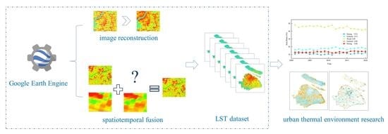
Figure 2.
The flowchart of LST production processing and thermal environment analysis.

Figure 3.
Simulation verification of accuracy. (a) Original LST, 19 May 2008. (b) Reconstructed LST, 19 May 2008. (c) Original LST, 20 July 2017. (d) LST by spatiotemporal fusion, 20 July 2017. (e) Original LST 26 July 2018. (f) LST after adding the gaps, 26 July 2018. (g) Reconstruction followed by spatiotemporal fusion for 26 July 2018. The content in the black box on the left of each part of the figure is enlarged as shown on the right.

Figure 4.
Number of high-quality existing Landsat LST images vs. number of generated filtered Landsat-like LST images. The Landsat LST images all have cloud coverage below 20%, and the Landsat-like LST images all have completeness above 90%.
Figure 4.
Number of high-quality existing Landsat LST images vs. number of generated filtered Landsat-like LST images. The Landsat LST images all have cloud coverage below 20%, and the Landsat-like LST images all have completeness above 90%.

Figure 5.
Plots of mean and trend changes of LST over the period 2001–2020. (a) Interannual and four-season averages and the results of the linear fit trend. (b–f) Interannual, spring–summer–autumn–winter mean changes and the trend results of the M–K test, respectively. UF and UB are the measures of positive and negative trends in the M–K statistic, respectively. UF > 0 indicates a continuous growth trend, and UF > confidence level (1.96) indicates a significant trend growth. It shows an abrupt change when UF intersects with UB.

Figure 6.
Seasonal UHI spatiotemporal trend maps. (A1–D5) represents the UHI grade maps for each season (spring, summer, autumn, winter) in different years. (E1–E5) illustrates the seasonal variation trends of UHI for individual years. (F1–F4) displays the UHI trend changes over the years for each individual season.

Figure 7.
Area ratios by Strong and General UHI to total area.

Figure 8.
Distribution of annual average UHI changes in Shanghai and 20-year trend change map.

Figure 9.
The area ratio of each UHI level to the total study area.

Figure 10.
Average UHII level (a) and LST (b) on different land use types.

Figure 11.
The proportion of each UHI level on different land use types in 2001 (a) and 2020 (b).

Figure 12.
Correlation between LST and NDVI, NDWI, and NDBI for 2001–2020.


Table 1.
Selected input images for spatiotemporal fusion.
| Date | Sensors Data | |
|---|---|---|
| 14 June 2000 | Landsat 7 ETM+ | MOD11A1 |
| 23 August 2002 | Landsat 7 ETM+ | MOD11A1 |
| 20 February 2005 | Landsat 7 ETM+ | MOD11A1 |
| 16 September 2005 | Landsat 7 ETM+ | MOD11A1 |
| 6 July 2008 | Landsat 7 ETM+ | MOD11A1 |
| 1 September 2011 | Landsat 7 ETM+ | MOD11A1 |
| 1 May 2013 | Landsat 7 ETM+ | MOD11A1 |
| 21 April 2015 | Landsat 7 ETM+ | MOD11A1 |
| 26 January 2016 | Landsat 8 TIRS | MOD11A1 |
| 13 February 2017 | Landsat 8 TIRS | MOD11A1 |
| 15 January 2018 | Landsat 8 TIRS | MOD11A1 |
| 12 May 2020 | Landsat 8 TIRS | MOD11A1 |
| 29 April 2021 | Landsat 8 TIRS | MOD11A1 |
Table 2.
Classification of UHI classes.
| UHI Rating | Threshold Range |
|---|---|
| Strong UHI | LST > μ + x |
| General UHI | μ + 0.5x ≤ LST ≤ μ + x |
| Weak UHI | μ − 0.5x < LST < μ + 0.5x |
| General UCI | μ − x ≤ LST ≤ μ − 0.5x |
| Strong UCI | LST < μ − x |
Table 3.
Accuracy evaluation results.
| Quantitative Metrics | (a)–(b) | (c)–(d) | (e)–(g) |
|---|---|---|---|
| RMSE (°C) | 4.33 | 1.78 | 2.33 |
| PSNR | 27.59 | 33.24 | 31.53 |
| CC | 0.86 | 0.96 | 0.93 |
Root Mean Square Error (RMSE). Peak Signal to Noise Ratio (PSNR). Correlation Coefficient (CC).
Table 4.
Contribution of different land use types to LST.
| Year | Parametric | Impervious | Forest-Grassland | Cropland | Water |
|---|---|---|---|---|---|
| 2001 | P (%) | 14.1 | 22.5 | 54 | 9.4 |
| C (°C) | 0.61 | −0.17 | 0.39 | −0.37 | |
| 2005 | P (%) | 18.3 | 23.5 | 47.6 | 10.5 |
| C (°C) | 0.8 | −0.22 | 0.35 | −0.41 | |
| 2010 | P (%) | 23.6 | 22.7 | 42.5 | 11.1 |
| C (°C) | 1.03 | −0.27 | 0.31 | −0.43 | |
| 2015 | P (%) | 26.2 | 22.2 | 40.4 | 11.2 |
| C (°C) | 1.14 | −0.31 | 0.29 | −0.44 | |
| 2020 | P (%) | 28 | 21.1 | 39.5 | 11.3 |
| C (°C) | 1.22 | −0.25 | 0.29 | −0.44 | |
| DT (°C) | 4.354 | −1.18 | 0.726 | −3.9 | |
The “DT” column represents the temperature difference between the average temperature of each land use type and the five-year image average temperature. Here, “P” represents the proportion of each land type, while “C” represents the contribution of each land type to the surface temperature. C = DT P.
Disclaimer/Publisher’s Note: The statements, opinions and data contained in all publications are solely those of the individual author(s) and contributor(s) and not of MDPI and/or the editor(s). MDPI and/or the editor(s) disclaim responsibility for any injury to people or property resulting from any ideas, methods, instructions or products referred to in the content. |
© 2023 by the authors. Licensee MDPI, Basel, Switzerland. This article is an open access article distributed under the terms and conditions of the Creative Commons Attribution (CC BY) license (https://creativecommons.org/licenses/by/4.0/).
Share and Cite
MDPI and ACS Style
Wang, M.; Lu, H.; Chen, B.; Sun, W.; Yang, G. Fine-Scale Analysis of the Long-Term Urban Thermal Environment in Shanghai Using Google Earth Engine. Remote Sens. 2023, 15, 3732. https://doi.org/10.3390/rs15153732
AMA Style
Wang M, Lu H, Chen B, Sun W, Yang G. Fine-Scale Analysis of the Long-Term Urban Thermal Environment in Shanghai Using Google Earth Engine. Remote Sensing. 2023; 15(15):3732. https://doi.org/10.3390/rs15153732
Chicago/Turabian StyleWang, Mengen, Huimin Lu, Binjie Chen, Weiwei Sun, and Gang Yang. 2023. "Fine-Scale Analysis of the Long-Term Urban Thermal Environment in Shanghai Using Google Earth Engine" Remote Sensing 15, no. 15: 3732. https://doi.org/10.3390/rs15153732
Note that from the first issue of 2016, this journal uses article numbers instead of page numbers. See further details here.