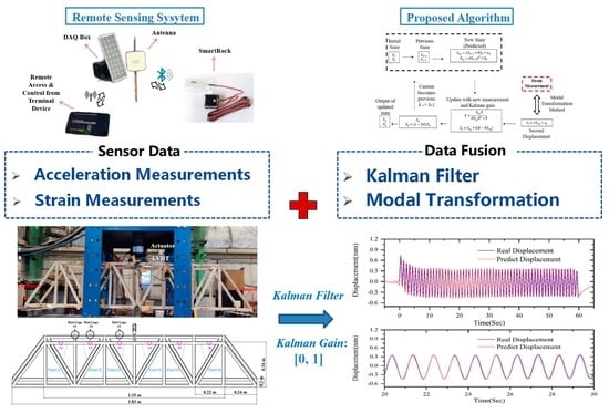
Sensing Mechanism and Real-Time Bridge Displacement Monitoring for a Laboratory Truss Bridge Using Hybrid Data Fusion

Abstract

Remote and real-time displacement measurements are crucial for a successful bridge health monitoring program. Researchers have attempted to monitor the deformation of bridges using remote sensing techniques such as an accelerometer when a static reference frame is not available. However, errors accumulate throughout the double-integration process, significantly reducing the reliability and accuracy of the displacement measurements. To obtain accurate reference-free bridge displacement measurements, this paper aims to develop a real-time computing algorithm based on hybrid sensor data fusion and implement the algorithm via smart sensing technology. By combining the accelerometer and strain gauge measurements in real time, the proposed algorithm can overcome the limitations of the existing methods (such as integration errors, sensor drifts, and environmental disturbances) and provide real-time pseud-static and dynamic displacement measurements of bridges under loads. A wireless sensor, SmartRock, containing multiple sensing units (i.e., triaxial accelerometer and strain gauges) and a Micro Controlling Unit (MCU) were utilized for remote data acquisition and signal processing. A remote sensing system (with SmartRocks, an antenna, an industrial computer, a Wi-Fi hotspot, etc.) was deployed, and a laboratory truss bridge experiment was conducted to demonstrate the implementation of the algorithm. The results show that the proposed algorithm can estimate a bridge displacement with sufficient accuracy, and the remote system is capable of the real-time monitoring of bridge deformations compared to using only one type of sensor. This research represents a significant advancement in the field of bridge displacement monitoring, offering a reliable and reference-free approach for remote and real-time measurements.

1. Introduction

Bridges and building infrastructure can generate dynamic displacement under external excitation, like cars, trains, and winds. Obtaining accurate, stable, and reliable displacement measurements is a crucial component of a successful structural health monitoring program for bridge maintenance [1,2]. In the past few decades, considerable efforts have been made toward sensors for the measurement of bridge dynamic responses under loads, such as the maximum deflection and dynamic deformation. Depending on how the sensor is used for measuring structural displacements, bridge structural displacement monitoring can be classified as direct method (e.g., total stations, LVDT, and camera) and indirect method (e.g., accelerometer, strain gauge, and inclinometer) sensors.

Among the direct methods, the linear variable differential transducer (LVDT) can provide real-time displacement measurements by connecting a measurement point and a reference point physically. It has a significant advantage over other forms of displacement transducers in terms of robustness and unlimited resolution. However, this approach is inconvenient and limited, particularly for bridges where the measurement point is too far away from the reference point [3,4]. Advancements in digital image correlation (DIC) techniques have enabled precise measurements of displacements based on high-resolution visual data [5]. Barros et al. conducted dynamic displacement measurements on a masonry rail bridge using 3D-DIC, discussing strategies to minimize on-site errors [6]. Nasimi and Moreu [7] developed a laser camera system mounted on an unmanned aerial vehicle to estimate the total transverse displacement on railroad bridges, achieving accuracy within a few millimeters.

Another direct method, a vision-based technique, like a high-speed and precision camera, can also be used for directly measuring structural displacement without requiring significant wiring [8,9]. Lee et al. introduced a dual-camera system that compensated for ego-motion, enabling the long-term monitoring of bridges [10]. They validated the system during the construction stages of a railway bridge girder. Xu et al. proposed an integrated approach that combined a deep learning-based Siamese tracker and correlation-based template matching, enhancing its robustness of the environmental conditions [11]. But it is hard to find a sensor installation location in many scenarios due to the device’s restricted range of measurement (no more than 200 m), and the device and the accuracy could easily be affected by the weather and other environmental disturbances.

As for indirect types of sensors, there have been many attempts to monitor the deflection of a bridge by using an inclinometer, strain gauge, fiber optics, accelerometer, etc. [12,13,14,15]. Among these, an accelerometer is the most commonly used sensor due to its characteristics of small size, easiness of deployment, and high signal resolution [16]. In addition, the effectiveness of employing acceleration for reconstructing dynamic displacement lies in its independence from the need for a reference point. Accelerometer data can be utilized to determine a bridge structure’s dynamic properties and can be converted into displacement through a double-integration process. However, the acceleration measurement contains small errors from sensor drifts, unknown initial conditions, and other noises. Using the direct double integration of acceleration to obtain displacements has to overcome an integration error that linearly accumulates during the integration process, which will produce a large error in the trend term [17,18,19,20]. To overcome these drawbacks, Lee et al. [21] suggested minimizing the drift error by removing low-frequency components below the first natural frequency. Moreu et al. [22] proposed a study to obtain the transverse displacement of a timber railroad bridge from acceleration by applying a finite impulse response (FIR) filter. The drift error is still hard to remove, because the FIR filter is more suitable in obtaining a transient response or sinusoidal response, as well as free vibration response, instead of pseudo-static displacements.

Recently, further research on improving bridge displacement monitoring based on the fusion of measurements from multi-sensors was also studied. Chan et al. [23] proposed an empirical mode decomposition (EMD)-based data fusion method that combined accelerometer and GPS measurements. An adaptive filter was then used to denoise the GPS displacement. EMD was used to fuse the high-frequency component of double-integrated acceleration with the denoised GPS displacement. However, EMD may introduce errors at the beginning and end of the processed signal, so longer records are needed to truncate these errors. Also, since EMD requires full-length measurements, it is not suitable for real-time displacement estimations. Hong et al. [24] developed a novel finite impulse response filter that combined acceleration and intermittent displacement measurements. While this approach showed promise, it required manual adjustment of the filter parameters, which limited its utility for automation. Kim et al. [25] proposed a displacement estimation system based on the fusion of an accelerometer and a RTK-GNSS. However, low-frequency noise in a RTK-GNSS signal was observed, which caused a high level of estimation errors in the results, and using RTK-GNSS makes it hard to monitor the displacement of a bridge in real time. It cannot provide time-synchronized measurements with acceleration measurements and will generate errors caused by interpolation. Zeng et al. [26] also introduced a method by fusing acceleration with gyroscope measurements. The ‘observation measurement’ in the iteration process of the Kalman filter was transferred from the angular rotation measurement. However, angular rotation could only be applied to simple structures such as cantilever beams and simply supported beams, and it was difficult to establish the mathematical and physical relationship between rotation and deformation for slightly more complex bridges. Moreover, the gyroscope provides the angular velocity measurement, which still requires integration to obtain displacement, resulting in drift errors in the long-term displacement measurement.

Therefore, it is clear that the current structural displacement monitoring methods have their limitations in obtaining accuracy and reference-free bridge displacement in real time. In this paper, a novel bridge reference-free displacement estimation algorithm is proposed and studied.

2. Objective, Novelty, and the General Framework

This paper aims to develop a smart computing algorithm and a bridge displacement monitoring system based on a hybrid sensors data fusion technique and verify their accuracy based on laboratory simulative tests. The key novelty of this paper lies in the development of a real-time bridge displacement monitoring system without the requirement of a fixed static reference point (so-called reference-free) based on hybrid sensor data fusion. By combining accelerometers and strain gauge measurements in real time, the proposed algorithm can overcome the limitations of the existing methods (such as integration errors, sensor drifts, and environmental disturbances) and provide real-time pseudo-static and dynamic displacement measurements of bridges under loads.

The framework of the proposed bridge displacement monitoring system consists of two parts: (1) a real-time computing algorithm based on data fusion techniques using the combination of acceleration and strain measurements and (2) a prototype smart sensor, SmartRock, enclosing multiple sensing units, i.e., a triaxle accelerometer, strain gauges, and a Micro Controlling Unit (MCU), which can execute the built-in smart computing algorithm in real time. In this paper, a series of laboratory simulation tests using SmartRocks on a model truss bridge was developed to evaluate the performance of the proposed algorithm and the SmartRocks. The real-time displacements obtained from the sensors and their built-in algorithm are further compared with real displacements from dial gauges and LVDT to validate the efficiency and accuracy of the sensor and the proposed algorithm.

3. Instrumentation

A remote sensing system (see Figure 1) was deployed for this study, which enables automatic data gathering, real-time data processing, remote data transmission, etc. [27]. The system includes several SmartRock sensors, an industrial computer for local data storage, an antenna for remote control and data collection, a Wi-Fi hotspot, and a data acquisition (DAQ) box equipped with a solar/battery kit. In this study, the battery was fully charged, so the solar panel was not utilized. Figure 1 provides a depiction of the system. The SmartRock can transmit the data through Bluetooth, and the terminal user can remotely access the data using any terminal device.

SmartRock (see Figure 2 [28]) is a wireless sensor containing multiple sensing units (i.e., triaxial accelerometer, gyroscope, and strain unit) and a Micro Controlling Unit (MCU) for executing the built-in smart computing algorithm. It can easily be installed on the surface of a bridge for real-time data acquisition and displacement estimations. It has the capability of recording triaxial acceleration and strain measurements in a time-synchronized manner at a high sampling rate (maximum 200 Hz). In this study, a total of six SmartRocks were utilized for real-time data acquisition, and the novel bridge deformation estimation algorithm proposed in this study was programmed in the SmartRock for real-time bridge deformation monitoring.

4. Methodology

One approach to obtaining reference-free deformation measurements is through the double integration of acceleration, although this method is subject to significant low-frequency drift errors [29]. Many attempts have been made to apply high-pass filters, but these attempts can negatively impact the accuracy of the results by removing true low-frequency components. In this study, Kalman filter was used to integrate the acceleration and strain measurements to produce a more accurate and robust estimate of the displacement while preserving the true low-frequency components [30]. Kalman filter [31] is an algorithm that uses a series of measurements observed over time, including statistical noise and other inaccuracies, and produces estimates of unknown variables that tend to be more accurate than those based on a single measurement alone by estimating the joint probability distribution over the variables for each time frame [32,33]. The proposed algorithm is depicted in a flowchart in Figure 3, and its methodology is described in detail as follows.

4.1. Formulation of Kalman Filter-Based Displacement Estimation Algorithm

The Kalman filter applied to the acceleration measurement is based on the state prediction model at a kth time step:

$${\mathit{x}}_{\mathit{k}}=A{·\mathit{x}}_{\mathit{k}-\mathbf{1}}+B{·u}_k+w_k$$

(1)

$$Z_k=h{·z}_k+v_k$$

(2)

where $\mathit{A}=\left[\begin{array}{cc}1& ∆t\\ 0& 1\end{array}\right]$, $\mathit{B}=\left[\begin{array}{c}\frac{1}{2}{∆t}^2\\ ∆t\end{array}\right]$, ${\mathit{x}}_{\mathit{k}}=\left[\begin{array}{c}{x}_k\\ \dot{x_k}\end{array}\right]$, $x_k$ is the displacement, $\dot{x_k}$ is the velocity, $u_k$ is the measured acceleration, $Z_k$ is an observation measurement with noise (here is the second displacement measurement in addition to $d_k$) at time k, $z_k$ is the sencond measurement, $∆t$ is the length of the time step, h is the observation model mapping the state prediction onto the observed state, $w_k$ is the white Gaussian noise of displacement regarding to the covariance, and $Q_k$ is also the white Gaussian noise regarding the second displacement measurement with the covariance $R_k$. These noises can be obtained by

$$Q_k=E(w_k,{w_k}^T),R_k=E(v_k,{v_k}^T)$$

(3)

where E is the mathematical expectation. The state-space model in Equations (1) and (2) is utilized to develop the Kalman filter-based displacement estimation algorithm, which can be separated into time update and measurement update steps:

• Time update

  a.

  Project the state ahead:

  $${{\mathit{x}}_{\mathit{k}}}^{-}=\mathit{A}{\mathit{x}}_{\mathit{k}-\mathbf{1}}+\mathit{B}{u}_k$$

  (4)

  b.

  Project the covariance ahead:

  $${P_k}^{-}=\mathit{A}{\widehat{P}}_{k-1}{\mathit{A}}^T+Q_k$$

  (5)

• Measurement update

  a.

  Compute the Kalman gain:

  $$K_k={P_k}^{-}{H}_k^T(H_k{P_k}^{-}{H}_k^T+R_k)$$

  (6)

  b.

  Update state estimate:

  $${\mathit{x}}_{\mathit{k}}={{{\mathit{x}}_{\mathit{k}}}^{-}+K}_k(Z_k-{{\mathit{x}}_{\mathit{k}}}^{-})$$

  (7)

  c.

  Update the covariance:

  $${\widehat{P}}_k=(I-K_{k}H){P_k}^{-}$$

  (8)

In the algorithm, the time update step puts forward the current state ${\mathit{x}}_{\mathit{k}-\mathbf{1}}$ and covariance ${\widehat{P}}_{k-1}$ to obtain an a priori displacement estimate ${x_k}^{-}$ based on the integration of acceleration and the initial state of the previous estimation ${\mathit{x}}_{\mathit{k}-\mathbf{1}}$. Then, in the measurement update step, the priori estimate ${{\mathit{x}}_{\mathit{k}}}^{-}$ is incorporated with an observation measurement $Z_k$ from a second monitoring tool to obtain an improved and accurate posterior estimate (proposed displacement). Therefore, finding a reliable ‘observation measurement’ $Z_k$ is the key component.

4.2. Strain–Displacement Transformation

In this study, strain gauges and a numerical finite element (FE) model transformation approach were used to obtain the ‘observation measurement’. The model transformation approach is based on modal superposition. This approach is generally utilized for the generation of the relationship between displacement and strain and estimating displacement using only a limited set of strain measurements [34,35,36]. In this approach, displacements of structures can be calculated from strain measurements using a series of selected mode shapes $\phi$ and strain mode shapes $\varphi$. As shown in Equations (9) and (10), both displacement $x$ and strain $\epsilon$ can be multiplied with the corresponding modal coordinate vector q, where N is the number of displacements at certain positions, n is the number of selected modes, M is the number of the measured strains, and the symbol $·$ is the matrix multiplication.

$${\left[d\right]}_{M\times 1}={\left[\phi \right]}_{M\times n}·{\left[q\right]}_{n\times 1}$$

(9)

$${\left[\epsilon \right]}_{M\times 1}={\left[\varphi \right]}_{N\times n}·{\left[q\right]}_{n\times 1}$$

(10)

Since the modal coordinate vector q is the same for the strain $\epsilon$ and the displacement $d$, the strain can be transformed into displacement in terms of the mode shape matrix and the strain mode shapes matrix as

$${{\left[d\right]}_{M\times 1}=\left[\phi \right]}_{M\times n}·\left({\left[\varphi \right]}_{N\times n}^T{·\left[\varphi \right]}_{N\times n}^{-1}·{\left[\varphi \right]}_{N\times n}^T\right)·{\left[\epsilon \right]}_{M\times 1}$$

(11)

where ${\left[\phi \right]}_{M\times n}·\left({\left[\varphi \right]}_{N\times n}^T{·\left[\varphi \right]}_{N\times n}^{-1}·{\left[\varphi \right]}_{N\times n}^T\right)$ is expressed as the strain-to-displacement transformation (SDT) matrix. Then, the displacement-to-strain relationship can be expressed as

$${\left[d\right]}_{M\times 1}={\left[SDT\right]}_{M\times N}·{\left[\epsilon \right]}_{n\times 1}$$

(12)

Hence, by combining acceleration and strain-transferred displacement measurements, the displacement of the structure at the sensor locations can be estimated.

4.3. Obtaining Full-Field Displacement

To obtain an accurate displacement measurement at other locations where no sensor is installed and project the full-field displacement of the upper chord, the modal expansion method is utilized [37,38].

Based on Equation (9), any response of the bridge could be obtained by a linear combination of the mode shapes $\phi$ with the weighing of modal coordinates q: ${\left[x\right]}_{M\times 1}={\left[\phi \right]}_{M\times n}·{\left[q\right]}_n$. M is the number of strain gauges (control nodes), and n is the number of modes (here, it is 4, based on the results in Section 4.2). This is called modal decorrelation. We calculated the modal coordinates q by transforming the nodal predicted displacement using modal decorrelation.

$${\left[q\right]}_n={\phi }_{M\times n}^{⊺}·{\left[d\right]}_{M\times 1}$$

(13)

where ${·}^{⊺}$ denotes the Moore–Penrose inverse. If we have the full-field mode matrix ${\left[\phi \right]}_{all\_node\times n}$ (all_node is the number of nodes in the FEM model), the full-field measurements of the system $\widehat{d}\left(t\right)$ can be obtained by replacing the spatial limited-mode matrix ${\left[\mathsf{\phi }\right]}_{\mathrm{M}\times \mathrm{n}}$ with the full-field mode matrix ${\left[\mathsf{\phi }\right]}_{\mathrm{a}\mathrm{l}\mathrm{l}\_\mathrm{n}\mathrm{o}\mathrm{d}\mathrm{e}\times \mathrm{n}},$ including all DOFs.

$$\widehat{d}\left(t\right)={\left[\phi \right]}_{all\_node\times n}·{\left[q\right]}_n={\left[\phi \right]}_{all\_node\times n}·{\phi }_{M\times n}^{⊺} ·{\left[d\right]}_{M\times 1}$$

(14)

5. Implementation and Verification of the Algorithm

5.1. Experimental Setup and Sensing Units

A laboratory-scale experiment was conducted to explain the implementation of the algorithm for displacement measurements and verify the performance and reliability of the SmartRock with a built-in smart computing algorithm. A G-Scale (1:22.5) wood truss bridge (Figure 4a) using dry lumber with a cross-section of 19.05 mm × 19.05 mm was constructed. The bridge had eight panels with a total span of 1.83 m, and all the truss members were screw-connected. The detailed dimensions of the bridge can be found in Figure 4b. The load was vertically applied through an actuator at the middle of the upper chord with a maximum capacity of 4500 N, and a harmonic load with a frequency of 1 Hz was applied as the test load.

Figure 4b presents a schematic diagram of the bridge and sensor installation plan. A total of six SmartRocks connected to six strain gauges were utilized to estimate the deflection of the top chord. The acceleration and strain were measured at the locations of SR1 to SR6. Three dial gages and a LVDT were used: dial gage #1 was mounted at the connection of panels #1 and #2, dial gage #2 was mounted at the middle of panel #2, and dial gage #3 was mounted at the middle of panel #3. The LVDT was mounted on the actuator.

The strain gauges used were linear type strain gauges with a high accuracy (noise level was ±0.5 με) and low sensitivity to temperature. They were prewired and easy to install. The vertical acceleration and the strain gauge measurements were imported into the built-in smart computing algorithm through the MCU to estimate the reference-free displacement of the upper chord of the truss bridge. The displacements recorded by three dial gages and LVDT at the middle of the upper chord were taken as the references to evaluate the accuracy of the estimated displacements.

5.2. Implementation of the Algorithm

Both the acceleration and strain measurements at the corresponding six locations were recorded by the SmartRocks in real time with a sample rate of 100 Hz. Figure 5 shows an example of the recorded acceleration and strain signals at the location of S3. Then, they were imported into the proposed algorithm for real-time computing. The procedure and results of the application are discussed in the following sections.

As mentioned earlier in Section 4.2, the strain gauges and model transformation approach were used to obtain the ‘observation measurement’ in the algorithm. According to Equation (12), it is possible to obtain the displacement and the observation measurement during the iteration of smart computing by multiplying the strain data by a displacement–strain relationship matrix (SDT). In the lab test application, the mode shapes and strain mode shapes need to be calculated first to construct the SDT matrix. A FE model of the truss bridge was constructed using the MATLAB Partial Differential Equation (PDE) toolbox [39]. The FEM model was built with meticulous attention to detail, considering the structural characteristics and geometry of the truss bridge. It consisted of a substantial number of linear tetrahedral elements, specifically 425,737, which were used to discretize the bridge’s geometry and represent its behavior under different loading conditions. To ensure the accuracy and reliability of the FEM model, it was calibrated using strain measurements obtained from strain gauges installed at specific locations on the truss bridge. By comparing the strain values predicted by the FEM model to the actual measured strains, adjustments and fine-tuning were made to optimize the model’s performance and ensure its compatibility with the experimental data. By solving the eigenvalue problem associated with the FEM model, the eigenfrequencies (natural frequencies) and corresponding mode shapes of the truss bridge were obtained. The obtained mode shapes represented the deformation patterns of the truss bridge at its natural frequencies. These mode shapes were visualized using contour plots, and in this case, the contour plots of the first eight mode shapes are shown in Figure 6. Additionally, strain mode shapes were also extracted from the FEM model. These strain mode shapes represented the spatial distribution of strains experienced by the truss bridge at its natural frequencies. The strain mode shapes were obtained by associating the modal displacements with strain values calculated using appropriate strain–displacement relationships. Both the mode shapes and strain mode shapes were crucial inputs for generating the SDT matrix.

It was important to include all the modes that contributed significantly to the deformation of the bridge into the transformation matrix to improve the accuracy of the strain-transferred displacements under a certain pattern of loads [28]. It was apparent from Figure 6 that mode 6 had the highest magnitude of mode deflection in the vertical direction. But, in order to reconstruct the deformation of the structure as thoroughly as possible, other modes could also be included. Therefore, a mode selection scheme [40] was applied before generating the SDT, and the process will be discussed as follows.

First, a static finite element analysis was conducted with a point vertical load at the same load location as in the lab test. The displacements δ from the static analysis results were used for the calculation of hybrid strain energy, as shown in Equations (15)–(18). Then, the mass-normalized modes were calculated through the result of the eigenvalue analysis; first, a static finite element analysis was conducted with a point vertical load at the same load location as in the lab test.

$$\psi =\frac{\phi }{\sqrt{{\phi }^T·\left[M\right]·\phi }}$$

(15)

where $\mathsf{\psi }$ is the mass-normalized mode shape, and $\mathrm{M}$ is the global mass matrix. Next, displacement from the static analysis was utilized to obtain the optimal modes using

$$q^i={{[\psi }^i]}^T·\left[M\right]·\delta$$

(16)

where $q^i$ is a combined modal coordinate for the ith mode, ${\psi }^i$ is the ith mode shape, and $M$ is the global mass matrix. The hybrid modal displacement for all the modes was then written as

$$\left[{\delta }_m\right]=\mathsf{\Sigma }{q}^i·{[\psi }^i]$$

(17)

Finally, the strain energy $E_m$ corresponding to the hybrid displacement was calculated as

$$\left[E_m\right]=\frac{1}{2}{{\delta }_m}^T·\left[K\right]·\left[{\delta }_m\right]$$

(18)

where K is the global stiffness matrix. The calculations performed in Equation (18) were for the total energy summed over the mode m. By examining the percents of the hybrid strain energies of each mode, it was feasible to identify how many modes should be included in the solution.

The first 20 modes were considered, and their hybrid strain energies for the lab-scaled truss bridge are shown in

Table 1. Hybrid strain energy percentages of the first 20 modes.

Mode Number	Strain Energy (N·m)	Ratio	Mode #	Strain Energy (N·m)	Ratio
1	1.70 × 108	10.1%	11	4.85 × 104	0.0%
2	8.20 × 104	0.0%	12	1.22 × 105	0.0%
3	4.90 × 105	0.0%	13	8.45 × 107	5.0%
4	4.66 × 106	0.3%	14	1.35 × 103	0.0%
5	3.18 × 104	0.0%	15	5.41 × 105	0.0%
6	1.32 × 109	78.6%	16	9.86 × 105	0.1%
7	5.80 × 105	0.0%	17	5.24 × 106	0.3%
8	5.31 × 104	0.0%	18	1.28 × 105	0.0%
9	1.52 × 106	0.1%	19	4.13 × 106	0.2%
10	3.41 × 106	0.2%	20	3.74 × 107	2.2%

. It should be noted that, when selecting mode shapes and constructing the SDT matrix, the rank of SDT (n) should be smaller than the number of strain sensors (M) used for estimating the deformed shapes accurately at the higher frequency excitation [41,42]. The ratios of modes 1, 6, 13, and 20 were 10.1%, 78.6%, 5.0%, and 2.2%, respectively, contributing to 95.9% of the total energy combined. Therefore, modes 1, 6, 13, and 20 were used to construct the SDT matrix. In this case, the SDT contained six rows (the number of strain gauges) and four columns (the number of modes). The measured strain values at the corresponding points (S1 to S6) and the SDT were substituted into Equation (12), which yielded strain-transferred displacements at the corresponding locations (See Figure 7). Then, the transferred displacement at the middle point of the top chord was obtained using the polynomial interpolation method for sensor fusion calculations. Figure 8 shows the comparison of strain-transferred displacements and real displacements at the locations of dial gage #2 and dial gage #3.

Figure 8 shows that the strain measurements could yield displacements that closely matched the real displacements in harmonic trend but not in magnitude. The accuracy was quantified by calculating the root mean square deviation (RMSD), as shown in Equation (19).

$$RMSD\left(\mathrm{\%}\right)=\frac{\sqrt{\sum {(x_{esitamete}-x_{real})}^2}}{\sqrt{\sum {x_{real}}^2}}\times 100$$

(19)

The peak displacements of the strain-transferred displacement and real displacement at each load cycle were selected for the RMSD calculations. The results were 16.48% at the location of dial gage #2 and 14.53% at the location of dial gage #3, which were not accurate enough in terms of the displacement monitoring accuracy requirements to a few tenths of a millimeter.

5.3. Displacement Prediction Using the Proposed Algorithm

In order to improve the accuracy and obtain a reliable bridge structural displacement prediction, the acceleration and strain measurements recorded by the SmartRocks were projected into the built-in smart computing algorithm for real-time computing. The effectiveness of the algorithm was investigated both at the locations with and without a sensor installed.

5.3.1. Predicting Displacements at Sensor Locations

With the acceleration measurements and strain-transferred displacements ready, the predicted displacements at the sensor locations (S1–S6) under the harmonic load were calculated using the proposed algorithm. As described in Section 4, in the time update step, it predicted a pre-state estimation ${x_k}^{-}$ at iteration step k based on the kinematic model defined in Equation (4) with the filtered acceleration and the predicted displacement $x_{k-1}$ and velocity $\dot{x_{k-1}}$ at step k−1 as the initial conditions. Then, the post-estimate of the displacement was obtained as a weighted linear summation of the pre-estimate of the state vector and the strain-transferred displacement $Z_k$. A comparison between the real displacements and the predicted displacements at the location of S2 was first plotted (see Figure 9) to verify the accuracy of the proposed algorithm at the sensor locations (where the accelerometers and strain gauges were installed).

As shown in Figure 9, the predicted displacements at the location of dial gage #2 showed good consistency with the real displacements (read from the corresponding dial gages) in both harmonic trend and displacement magnitude. Similar good agreements were observed for the locations of dial gages #3, which are not presented herein. The RMSD of the predicted displacements at these two observed sensor locations were calculated and are shown in

Table 2. RMSD of strain-transferred displacement and predicted displacement corresponding to real displacement.

Location	RMSD
	Strain-Transferred Displacement	Predicted Displacement
Dial gage #2	16.48%	4.91%
Dial gage #3	14.53%	4.25%

.

Table 2 shows that the predicted displacements had lower RMSD values than the strain-transferred displacements for the two locations. Considering many unknown disturbances from the environment and the sensors, the RMSD of the predicted displacements apparently demonstrated good performance of the proposed method. Therefore, the capability of the proposed bridge displacement estimation algorithm in obtaining an accurate bridge displacement with the fusion of acceleration and strain measurements at the location where the strain gauge and accelerometer were installed was validated.

5.3.2. Predicting Displacements at the Location without a Sensor Installed

Using the modal expansion method (Equations (13) and (14)) and the predicted displacements at the control nodes (in a selected combination), displacement at any point on the upper chord could be estimated. In addition, to investigate the effects of sensor location and projecting the most accurate full-field displacement measurements of the truss upper chord, three pairs of strain gauges and SmartRocks in different control node combinations were studied. Considering that the bridge was symmetrical, a total of nine combination cases were considered: Cases 124, 125, 126, 135, 136, 236, 245, 345, and 346, and the numbers correspond to sensor serial numbers in Figure 2b. The numbers in the cases referred to the number of selected sensors (from SR1 to SR6). The results from the predicted displacements and the corresponding real displacements at the location of dial gage #1 (the connection of upper panels #1 and #2) and the LVDT (the middle of the upper chord) were used as the validation.

Figure 10 and Figure 11 depict the plots of the peak values of real displacement versus predicted displacement for nine different combination cases at the locations of dial gage #1 and the middle of the upper chord (the location of the LVDT). Considering that only three SmartRocks were selected, the predicted values showed a good match with the real displacements. However, the results indicated that the locations of the selected control nodes had an effect on the accuracy of the displacement estimations. The RMSD varied from 5.27% to 10.93% at the location of dial gage #1 and from 5.57% to 7.68% at the middle of the upper chord. The combination of 136, 245, and 345 showed better accuracy than the rest of the combinations. Among them, the displacements from the combinations of 136 were the closest to the real displacements at both validation locations and had the best overall RMSD values: 5.27% and 5.57%. Therefore, a hypothesis on the optimal control node locations for obtaining the most accurate overall predicted displacement could be obtained; of the three control nodes, two nodes should be symmetrical at about the middle of the upper chord, and the remaining one should be next to it.

To verify this hypothesis, the predicted displacements from the symmetry group of these three combinations (135 corresponding to 145, 245 corresponding to 235, and 345 corresponding to 234) were also estimated, and the results are plotted in Figure 12. The results showed a good accuracy, and still, the combination of 146, which corresponded to 135, had the best performance (RMSD: 5.83% and 5.45%). Thus, the optimum combination of control nodes for obtaining an accurate displacement estimation of the upper chord was that two of the three control points should be symmetrical at about the middle of the upper chord and distributed at the extreme ends as much as possible, and the remaining one should be next to the center on either side.

6. Conclusions

In this paper, a novel algorithm based on real-time data fusion of the acceleration and strain measurements was developed to estimate the dynamic displacements of bridges without relying on a static reference frame. The algorithm was recursive and used noisy measurements observed over time from both of the sensor units, including statistical noise and other inaccuracies, and estimated the state of the bridge dynamics, which tends to be more accurate than the measurements based on only one type of sensor. A SmartRock, enclosing a triaxial accelerometer, multiple strain gauges, and a Micro Controlling Unit (MCU), was also developed to execute the real-time built-in algorithm. The sensor was applied to laboratory-scale wood truss bridge tests to estimate the dynamic displacement. The results were compared with the real displacement recordings by both the LVDT and dial gages to validate the accuracy and effectiveness of the proposed methodology. Based on the results of this study, the following conclusions were reached:

(1)

SmartRock with a built-in smart computing algorithm is capable of estimating bridge displacements in real time and can improve the accuracy compared to using only one type of sensor.

(2)

The predicted displacements using the proposed algorithm at the sensor locations (S1–S6) under a harmonic load showed a good match with the dial and gauge measured ‘real’ displacements in both harmonic trend and displacement magnitude. The RMSD of the predicted displacements were 4.91% and 4.25% at the two selected locations.

(3)

The modal expansion method was utilized to project the full-field displacements of the upper chord of the truss and yielded an excellent match with the real displacements.

(4)

The locations of the control nodes selected affected the accuracy of the displacement estimations when predicting the full-field displacements using three control nodes. The optimum combination of the control nodes for obtaining accurate displacement estimations of the upper chord was that two of the three control nodes should be symmetrical at about the middle of the upper chord and distributed at the extreme ends as much as possible, and the remaining one should be next to the center.

References

1. Lee, J.J.; Shinozuka, M. Real-time displacement measurement of a flexible bridge using digital image processing techniques. Exp. Mech. 2006, 46, 105–114. [Google Scholar] [CrossRef]
2. Huang, Q.; Monserrat, O.; Crosetto, M.; Crippa, B.; Wang, Y.; Jiang, J.; Ding, Y. Displacement monitoring and health evaluation of two bridges using Sentinel-1 SAR images. Remote Sens. 2018, 10, 1714. [Google Scholar] [CrossRef] [Green Version]
3. Joshi, S.; Harle, S.M. Linear variable differential transducer (LVDT) & its applications in civil engineering. Int. J. Transp. Eng. Technol. 2017, 3, 62–66. [Google Scholar]
4. Garg, P.; Nasimi, R.; Ozdagli, A.; Zhang, S.; Mascarenas, D.D.L.; Reda Taha, M.; Moreu, F. Measuring transverse displacements using unmanned aerial systems laser Doppler vibrometer (UAS-LDV): Development and field validation. Sensors 2020, 20, 6051. [Google Scholar] [CrossRef] [PubMed]
5. Curt, J.; Capaldo, M.; Hild, F.; Roux, S. An algorithm for structural health monitoring by digital image correlation: Proof of concept and case study. Opt. Lasers Eng. 2022, 151, 106842. [Google Scholar] [CrossRef]
6. Barros, F.; Aguiar, S.; Sousa, P.J.; Cachaço, A.; Tavares, P.J.; Moreira, P.M.; Ranzal, D.; Cardoso, N.; Fernandes, N.; Fernandes, R.; et al. Displacement monitoring of a pedestrian bridge using 3D digital image correlation. Procedia Struct. Integr. 2022, 37, 880–887. [Google Scholar] [CrossRef]
7. Nasimi, R.; Moreu, F. A methodology for measuring the total displacements of structures using a laser–camera system. Comput.-Aided Civ. Infrastruct. Eng. 2021, 36, 421–437. [Google Scholar] [CrossRef]
8. Olaszek, P.; Świercz, A.; Boscagli, F. The integration of two interferometric radars for measuring dynamic displacement of bridges. Remote Sens. 2021, 13, 3668. [Google Scholar] [CrossRef]
9. Lydon, D.; Lydon, M.; Taylor, S.; Del Rincon, J.M.; Hester, D.; Brownjohn, J. Development and field testing of a vision-based displacement system using a low cost wireless action camera. Mech. Syst. Signal Process. 2019, 121, 343–358. [Google Scholar] [CrossRef] [Green Version]
10. Lee, J.; Lee, K.C.; Jeong, S.; Lee, Y.J.; Sim, S.H. Long-term displacement measurement of full-scale bridges using camera ego-motion compensation. Mech. Syst. Signal Process. 2020, 140, 106651. [Google Scholar] [CrossRef]
11. Xu, Y.; Zhang, J.; Brownjohn, J. An accurate and distraction-free vision-based structural displacement measurement method integrating Siamese network based tracker and correlation-based template matching. Measurement 2021, 179, 109506. [Google Scholar] [CrossRef]
12. Xiao, F.; Chen, G.S.; Hulsey, J.L. Monitoring bridge dynamic responses using fiber Bragg grating tiltmeters. Sensors 2017, 17, 2390. [Google Scholar] [CrossRef] [PubMed] [Green Version]
13. Xiao, F.; Hulsey, J.L.; Balasubramanian, R. Fiber optic health monitoring and temperature behavior of bridge in cold region. Struct. Control Health Monit. 2017, 24, e2020. [Google Scholar] [CrossRef]
14. Won, J.; Park, J.W.; Park, J.; Shin, J.; Park, M. Development of a reference-free indirect bridge displacement sensing system. Sensors 2021, 21, 5647. [Google Scholar] [CrossRef]
15. Cai, C.; He, Q.; Zhu, S.; Zhai, W.; Wang, M. Dynamic interaction of suspension-type monorail vehicle and bridge: Numerical simulation and experiment. Mech. Syst. Signal Process. 2019, 118, 388–407. [Google Scholar] [CrossRef]
16. Zhuge, S.; Xu, X.; Zhong, L.; Gan, S.; Lin, B.; Yang, X.; Zhang, X. Noncontact deflection measurement for bridge through a multi-UAVs system. Comput.-Aided Civ. Infrastruct. Eng. 2021, 37, 746–761. [Google Scholar] [CrossRef]
17. Park, J.W.; Sim, S.H.; Jung, H.J. Development of a wireless displacement measurement system using acceleration responses. Sensors 2013, 13, 8377–8392. [Google Scholar] [CrossRef] [Green Version]
18. Ozdagli, A.I.; Liu, B.; Moreu, F. Low-cost, efficient wireless intelligent sensors (LEWIS) measuring real-time reference-free dynamic displacements. Mech. Syst. Signal Process. 2018, 107, 343–356. [Google Scholar] [CrossRef]
19. Thong, Y.K.; Woolfson, M.S.; Crowe, J.A.; Hayes-Gill, B.R.; Jones, D.A. Numerical double integration of acceleration measurements in noise. Measurement 2004, 36, 73–92. [Google Scholar] [CrossRef]
20. Ozdagli, A.I.; Gomez, J.A.; Moreu, F. Real-time reference-free displacement of railroad bridges during train-crossing events. J. Bridge Eng. 2017, 22, 04017073. [Google Scholar] [CrossRef]
21. Lee, H.S.; Hong, Y.H.; Park, H.W. Design of an FIR filter for the displacement reconstruction using measured acceleration in low-frequency dominant structures. Int. J. Numer. Methods Eng. 2010, 82, 403–434. [Google Scholar] [CrossRef]
22. Moreu, F.; Li, J.; Jo, H.; Kim, R.E.; Scola, S.; Spencer, B.F., Jr.; LaFave, J.M. Reference-free displacements for condition assessment of timber railroad bridges. J. Bridge Eng. 2016, 21, 04015052. [Google Scholar] [CrossRef]
23. Chan, W.S.; Xu, Y.L.; Ding, X.L.; Dai, W.J. An integrated GPS–accelerometer data processing technique for structural deformation monitoring. J. Geod. 2006, 80, 705–719. [Google Scholar] [CrossRef]
24. Hong, Y.H.; Lee, S.G.; Lee, H.S. Design of the FEM-FIR filter for displacement reconstruction using accelerations and displacements measured at different sampling rates. Mech. Syst. Signal Process. 2013, 38, 460–481. [Google Scholar] [CrossRef]
25. Kim, K.; Sohn, H. Dynamic Displacement Estimation for Long-Span Bridges Using Acceleration and Heuristically Enhanced Displacement Measurements of Real-Time Kinematic Global Navigation System. Sensors 2020, 20, 5092. [Google Scholar] [CrossRef] [PubMed]
26. Zeng, K.; Huang, H.; Song, S. Displacement Measurement Based on Data Fusion and Real-Time Computing. J. Perform. Constr. Facil. 2020, 34, 04020118. [Google Scholar] [CrossRef]
27. Zeng, K.; Qiu, T.; Bian, X.; Xiao, M.; Huang, H. Identification of ballast condition using SmartRock and pattern recognition. Constr. Build. Mater. 2019, 221, 50–59. [Google Scholar] [CrossRef]
28. Liu, S.; Qiu, T.; Qian, Y.; Huang, H.; Tutumluer, E.; Shen, S. Simulations of large-scale triaxial shear tests on ballast aggregates using sensing mechanism and real-time (SMART) computing. Comput. Geotech. 2019, 110, 184–198. [Google Scholar] [CrossRef]
29. Wang, C.; Li, Y.; Tran, N.H.; Wang, D.; Khatir, S.; Wahab, M.A. Artificial neural network combined with damage parameters to predict fretting fatigue crack initiation lifetime. Tribol. Int. 2022, 175, 107854. [Google Scholar] [CrossRef]
30. Khatir, S.; Tiachacht, S.; Thanh, C.L.; Tran-Ngoc, H.; Mirjalili, S.; Wahab, M.A. A robust FRF damage indicator combined with optimization techniques for damage assessment in complex truss structures. Case Stud. Constr. Mater. 2022, 17, e01197. [Google Scholar] [CrossRef]
31. Bishop, G.; Welch, G. An introduction to the kalman filter. In Proceedings of the SIGGRAPH, Los Angeles, CA, USA, 12–17 August 2001; Volume 8, p. 41. [Google Scholar]
32. Li, Y.; Cao, M.; Tran-Ngoc, H.; Khatir, S.; Wahab, M.A. Multi-parameter identification of concrete dam using polynomial chaos expansion and slime mould algorithm. Comput. Struct. 2023, 281, 107018. [Google Scholar]
33. Tran-Ngoc, H.; Khatir, S.; Le-Xuan, T.; Tran-Viet, H.; De Roeck, G.; Bui-Tien, T.; Wahab, M.A. Damage assessment in structures using artificial neural network working and a hybrid stochastic optimization. Sci. Rep. 2022, 12, 4958. [Google Scholar] [CrossRef] [PubMed]
34. Foss, G.C.; Haugse, E.D. Using modal test results to develop strain to displacement transformations. In Proceedings of the 13th International Modal Analysis Conference, Nashville, TN, USA, 13–16 February 1995; Volume 2460, p. 112. [Google Scholar]
35. Kang, L.H.; Kim, D.K.; Han, J.H. Estimation of dynamic structural displacements using fiber Bragg grating strain sensors. J. Sound Vib. 2007, 305, 534–542. [Google Scholar] [CrossRef]
36. Gherlone, M.; Cerracchio, P.; Mattone, M. Shape sensing methods: Review and experimental comparison on a wing-shaped plate. Prog. Aerosp. Sci. 2018, 99, 14–26. [Google Scholar] [CrossRef]
37. Yu, M.; Guo, J.; Lee, K.M. A modal expansion method for displacement and strain field reconstruction of a thin-wall component during machining. IEEE/ASME Trans. Mechatron. 2018, 23, 1028–1037. [Google Scholar] [CrossRef]
38. Bharadwaj, K.; Sheidaei, A.; Afshar, A.; Baqersad, J. Full-field strain prediction using mode shapes measured with digital image correlation. Measurement 2019, 139, 326–333. [Google Scholar] [CrossRef]
39. Mathworks Partial Differential Equation Toolbox. Available online: https://www.mathworks.com/products/pde.html (accessed on 1 January 2021).
40. Gonen, S.; Erduran, E. A Hybrid Method for Vibration-Based Bridge Damage Detection. Remote Sens. 2022, 14, 6054. [Google Scholar] [CrossRef]
41. Rapp, S.; Kang, L.H.; Han, J.H.; Mueller, U.C.; Baier, H. Displacement field estimation for a two-dimensional structure using fiber Bragg grating sensors. Smart Mater. Struct. 2009, 18, 025006. [Google Scholar] [CrossRef]
42. Cara, F.J.; Juan, J.; Alarcón, E.; Reynders, E.; De Roeck, G. Modal contribution and state space order selection in operational modal analysis. Mech. Syst. Signal Process. 2013, 38, 276–298. [Google Scholar] [CrossRef] [Green Version]
Figure 1. A photo of the remote sensing system.
Remotesensing 15 03444 g001
Figure 2. Photo of a SmartRock.
Remotesensing 15 03444 g002
Figure 3. Flowchart of the proposed algorithm.
Remotesensing 15 03444 g003
Figure 4. (a) Laboratory setup of the scaled wood truss bridge; (b) schematic diagram of the bridge and sensor installation plan.
Remotesensing 15 03444 g004
Figure 5. Signals measured at the middle point of panel #3 on the upper chord (location of S3): (a) acceleration; (b) strain.
Remotesensing 15 03444 g005
Figure 6. Modal shapes along the vertical direction of the lab truss bridge.
Remotesensing 15 03444 g006
Figure 7. Strain-transferred displacements at S1 to S6.
Remotesensing 15 03444 g007
Figure 8. Strain-transferred displacements at the locations of (a) dial gage #2 and (b) dial gage #3.
Remotesensing 15 03444 g008
Figure 9. Comparison of real displacement versus predicted displacement at the location of S2: (a) all-time series of data; (b) 10-s zoom-in time window.
Remotesensing 15 03444 g009
Figure 10. The peak values of real displacements versus predicted displacements from different control node combinations at the location of dial gage #1.
Remotesensing 15 03444 g010
Figure 11. The peak values of real displacements versus predicted displacements from different control node combinations at the middle of the upper chord.
Remotesensing 15 03444 g011
Figure 12. The peak values of real displacements versus predicted displacements from different combinations of control nodes: 146, 234, and 235 at the locations of (a) dial gage #1 and (b) the middle of the upper chord.
Remotesensing 15 03444 g012