2D-DOA Estimation in Multipath Using EMVS Rectangle Array

Abstract

Electromagnetic vector sensor (EMVS) arrays bring an epochal opportunity for direction finding, as they enable the estimation of two-dimensional direction of arrival (2D-DOA) and polarization characteristics. In this paper, we revisit the 2D-DOA estimation problem in an EMVS rectangle array under multipath propagation. An improved subspace estimator is proposed, which addresses the rank-deficit problem through matrix arrangement, and the 2D-DOA and polarization parameters are estimated via combining the normalized vector cross-product with the least squares method. Our proposed method is suitable for a single snapshot scenario and offers superior accuracy compared to existing methods. To validate its effectiveness, several numerical simulations have been designed and conducted.

1. Introduction

Array signal processing is a rapidly developing field, with direction of arrival (DOA) estimation being a particularly popular topic [1,2,3,4,5]. The goal of DOA estimation is to determine the direction of signal arrival by extracting the invariant phase difference between array elements from spatial information, among other factors. Several methods exist for DOA estimation, beginning with the early one-dimensional techniques such as signal subspace scaled Multiple Signal Classification (SSMUSIC) [6]. Although SSMUSIC provides high-resolution DOA estimation, it has a high computational complexity due to the process of searching for spectral peaks and handling subspace mismatch. Another one-dimensional technique is the coherent source DOA estimation algorithm based on Toeplitz matrix and estimation of signal parameter via rotational invariance techniques (ESPRIT) [7], which solves the problem of rank loss of the spatial covariance matrix caused by coherent signals. However, both SSMUSIC and ESPRIT are only applicable to uniform linear arrays. Compressed sensing-based DOA estimation algorithms [8] can solve the difficult underdetermined DOA estimation problem, but they are also limited to uniform linear arrays. Similarly, the MUSIC-Like algorithm [9] does not require prior knowledge of the number of sources, but its generalized eigendecomposition for each direction leads to high computational complexity. In contrast, practical two-dimensional DOA estimation techniques such as the propagator method (PM) for uniform linear arrays [10] and fast 2D-DOA estimation techniques for L-shaped arrays [11] provide efficient DOA estimation, but they are limited in applicability and not suitable for the sparse array structure required by the mainstream today. Another 2D-DOA estimation algorithm based on matrix reconstruction [12] can solve the 2D-DOA estimation problem of coherent sources, but its computational complexity is higher than that of general algorithms due to matrix reconstruction. Notably, all these methods use scalar sensors and disregard the polarization state of the signal.

Electromagnetic vector sensors (EMVSs) is a type of sensor based on the theory of electromagnetic fields, which can measure the electric and magnetic field strengths of electromagnetic waves in space and extract spatial information from the signals. Its basic principle is to use a receiving antenna array to measure the amplitude and phase information of the incident electromagnetic wave signal and then determine the direction of the incident signal. So emergence of EMVS has extended the field of signal processing beyond the traditional time, space and frequency domains to the polarization domain, where the polarization state is not only an inherent property of the electromagnetic wave but also carries important information about the signal. Unlike traditional scalar sensors, EMVSs have multiple components, such as electronic dipoles and magnetic loops, that can sense both electronic and magnetic field strengths simultaneously at a single point in space [4]. EMVS is typically composed of multiple channels, allowing for the simultaneous measurement of electromagnetic field components in different directions and polarization states. This enables the sensor to acquire more comprehensive polarization information. Additionally, EMVS can operate under different polarization modes, such as horizontal polarization, vertical polarization and oblique polarization. By utilizing different polarization modes, EMVS can provide additional information for the analysis and understanding of objects and environments within the electromagnetic field. Importantly, the sensor possesses the ability to suppress or minimize interference signals from non-target polarization states, thereby improving estimation accuracy. When the incident electromagnetic wave signal arrives at EMVS, there will be time and amplitude differences between signals received by different antennas. By measuring these differences, the direction of the incident signal can be determined. In addition to estimating DOA, EMVS demonstrates excellent performance in polarization estimation. This includes the ability to accurately estimate the polarization state of targets, such as linear polarization angle, circular polarization degree and ellipticity. EMVS can also distinguish subtle differences between different polarization states. Furthermore, it possesses polarization calibration capabilities, allowing the sensor to eliminate biases and non-linearities through a calibration process, ensuring consistency between the measured results and the actual polarization state. In practical applications, EMVS can be configured into different shapes and sizes of antenna arrays to meet the requirements of different application scenarios. The common construction methods of EMVS include linear arrays, circular arrays, rectangular arrays and so on. A linear array is typically composed of several equidistant receiving antennas and the spacing and number of antennas determine the direction diagram resolution and sensitivity of the array. A circular array is usually used to receive signals with uncertain directions and its direction diagram has rotational symmetry, which can receive a wider range of signal directions with the same sensitivity. A rectangular array has characteristics of both a linear array and a circular array in two dimensions and is suitable for signals with directional offsets. This paper constructs a rectangular array to estimate 2D-DOA. Due to their larger degree of freedom (DOF), EMVS arrays possess several valuable features, including strong anti-interference and detection abilities, as well as high resolution. Additionally, EMVS arrays have distinct polarization multi-access capabilities, making them more suitable for space-limited devices than scalar sensor arrays. In various military applications, such as radar, navigation and wireless communication and in some complex civil communication fields, polarization-sensitive arrays have begun to replace conventional antenna arrays. Notably, the combination of EMVS arrays and multi-input multi-output (MIMO) technology has led to a historic breakthrough in radar development. For example, the utilization of bistatic radar enables the acquisition of directional information and polarization state of Unmanned Aerial Vehicles (UAVs), facilitating their precise positioning [13]. Another application involves the imaging of automobiles using millimeter wave radar [14]. Furthermore, the use of the polarization domain enabled by EMVS has facilitated the further development of Synthetic Aperture Radar (SAR) Imaging [15] and Inverse SAR Imaging systems [16]. Compression sensing technology is one of the most crucial algorithms for imaging applications, as it compresses multi-dimensional data before reconstructing sparse images [17]. High-resolution source location is critical for the imaging applications mentioned above.

The tasks of 2D-DOA and polarization estimation are fundamental in EMVS array signal processing and have received considerable attention. Many excellent estimation algorithms have been developed, including based on rotation invariance techniques (ESPRIT) [18], an extension of ESPIRT, ESPRIT-Like algorithm [19], tensor-based approach [20,21] and spectrum grid search strategy [22,23]. Unfortunately, most of the existing works in this area are focused on non-coherent source issues, while in practice, multipath propagation often leads to coherent sources in wireless communications. Only a few efforts have been made to address the issue of coherent sources using EMVS arrays. In [24], a maximum likelihood (ML) estimator was reported, in which the multiple parameters in [24] were estimated in an iterative method and the estimator is computationally inefficient due to the slowness of convergence. In [25], the spatial smoothing (SS) algorithm was proposed, which utilizes spatial domain smoothing to eliminate the rank-deficiency of coherent sources in the measurement. The polarization smoothing (PS) strategy was suggested in [24], which restores the rank of the array measurement via averaging the measurement along the polarization domain. An improved PS approach was introduced in [26], whose smoothing procedure was implemented via a differential smoothing. However, the SS algorithm is only suitable for uniform array geometry and it suffers from aperture loss. The PS approach, however, is sensitive to the polarization parameter and it cannot provide polarization characteristics of the coherent sources. To be more specific, the contributions of this paper are listed as follows:

▪

We address the issue of 2D-DOA estimation for uniform rectangular array (URA). Unlike decorrelation methods in [24,25,26], the proposed algorithm utilizes matrix reordering for data preprocessing before decomposing the covariance matrix into a subspace. Moreover, under the same Uniform Rectangular Array (URA) structure, it is applicable to single-snapshot scenarios without loss of array effective aperture when the inter-element spacing is larger than the wavelength. So the proposed method outperforms the existing SS and PS methods.

▪

We propose a novel estimation approach for EMVS rectangle array. Different from [27,28], the proposed algorithm is based on reordering the array outputs, rather than reconstructing the signal covariance matrix, which significantly reduces the computational burden. It not only achieves automatic pairing of 2D-DOA, but also enables estimation of the polarization state simultaneously. The 2D-DOA and polarization characteristics are obtained via the vector cross product (VCP) and the least squares (LS) method. More importantly, the proposed algorithm achieves excellent estimation performance with a small number of snapshots, while maintaining stable estimation performance for uncorrelated, partially correlated and fully coherent signals.

▪

In our analysis, we examine the proposed algorithm in terms of identifiability, complexity and the Cramér–Rao Bound (CRB). Additionally, we conduct comprehensive computer simulations to validate the effectiveness of the algorithm.

Notations: we use ⊗, ⊙, ⊕ and ⊛ to symbolize, respectively, Kronecker product, Khatri–Rao product, Hadamard product and VCP. The superscripts ${(·)}^T$, ${(·)}^{-1}$, ${(·)}^{*}$ and ${(·)}^H$ represent transpose, inverse, conjugate and conjugate transpose, respectively. ${(·)}^{†}$ is pseudo-inverse. The $N\times N$ identity matrix is denoted by ${\mathit{I}}_N$ and ${\mathit{i}}_{N,n}$ denotes the n-th row of ${\mathit{I}}_N$; ${\mathbf{1}}_{N,M}$ stands for the all ones $N\times M$ matrix; $\mathcal{V}\left\{·\right\}$ and $diag\left\{·\right\}$ represent the vectorization and diagonalization; ${\mathcal{U}}_N\left(\right)$ denotes the operation of stacking a vector into an N-row matrix; $\delta \left(·\right)$ denotes the Kronecker delta; $real\left\{·\right\}$ and $Rank\left\{·\right\}$ return the real part and the rank of the matrix, respectively.

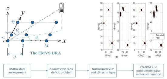
2. Signal Model of Polarized URA

Herein, we consider K far-field monochromatic transverse electromagnetic (TEM) source signals impinging on an $M\times N$ polarized uniform rectangular array (URA), as shown in Figure 1, and we assume that the URA lies on the x–o–y axis and each antenna consists of a colocated, completed EMVS. The inter-element spacing of the EMVS is d. The k-th source signal is parameterized by $\left\{{\theta }_k,{\varphi }_k,{\gamma }_k,{\eta }_k\right\}$, where ${\theta }_k$ denotes the elevation angle, ${\varphi }_k$ accounts for the azimuth angle, ${\gamma }_k$ stands for the auxiliary polarization angle and ${\eta }_k$ represents the polarization phase difference ($k=1,2,\cdots ,K$). The pair of angles $\left({\theta }_k,{\varphi }_k\right)$ is commonly referred to as the 2D-DOA of the k-th signal. The outputs of the URA, consisting of L snapshots, can be expressed as [29]

$$\begin{array}{ccc}\hfill \mathit{Y}& =& \left[{\mathit{A}}_x\odot {\mathit{A}}_y\odot \mathit{B}\right]{\mathit{S}}^T+{\mathit{N}}_{\mathrm{Y}}\hfill \\ & =& \left[{\mathit{A}}_x\odot {\mathit{B}}_y\right]{\mathit{S}}^T+{\mathit{N}}_{\mathrm{Y}},\hfill \end{array}$$

(1)

the array output $\mathit{Y}$ is represented as the Khatri–Rao product of the spatial response and polarization response of the sensor to the signal source, multiplied by the complex envelope of the signal and added to the form of additive Gaussian white noise, where ${\mathit{A}}_x=[{\mathit{a}}_{x,1},{\mathit{a}}_{x,2},\cdots ,{\mathit{a}}_{x,K}]$ with ${\mathit{a}}_{x,k}={\left[e^{-j2\pi ·0d{u}_k/\lambda },e^{-j2\pi d{u}_k/\lambda },\cdots ,e^{-j2\left(M-1\right)\pi d{u}_k/\lambda }\right]}^T$ denotes the k-th spatial response vector corresponding to the x-axis; ${\mathit{A}}_y=[{\mathit{a}}_{y,1},{\mathit{a}}_{y,2},\cdots ,{\mathit{a}}_{y,K}]$ with ${\mathit{a}}_{y,k}={\left[e^{-j2\pi ·0d{v}_k/\lambda },e^{-j2\pi d{v}_k/\lambda },\cdots ,e^{-j2\left(N-1\right)\pi d{v}_k/\lambda }\right]}^T$ denotes the k-th spatial response vector corresponding to the y-axis; $\mathit{B}=\left[{\mathit{b}}_1,{\mathit{b}}_2,\dots ,{\mathit{b}}_K\right]\in {\mathbb{C}}^{6\times K}$; $\mathit{S}=[{\mathit{s}}_1,{\mathit{s}}_2,\cdots ,{\mathit{s}}_K]$, ${\mathit{s}}_k={\left[s_{k,1},s_{k,2},\dots ,s_{k,L}\right]}^T$ denotes complex envelope of the k-th source signal; ${\mathit{N}}_{\mathrm{Y}}\in {\mathbb{C}}^{6NM\times L}$ denotes the additive noise measurement matrix; ${\mathit{B}}_y={\mathit{A}}_y\odot \mathit{B}$. In addition, the direction cosines are, respectively, defined as $u_k=cos\left({\varphi }_k\right)sin\left({\theta }_k\right)$, $v_k=sin\left({\varphi }_k\right)sin\left({\theta }_k\right)$. Moreover, the polarization response vector of the k-th source is expressed as follows

$${\mathit{b}}_k=\left[\begin{array}{c}cos{\theta }_{k}cos{\varphi }_{k}sin{\gamma }_k{e}^{j{\eta }_k}-sin{\varphi }_{k}cos{\gamma }_k\\ cos{\theta }_{k}sin{\varphi }_{k}sin{\gamma }_k{e}^{j{\eta }_k}+cos\varphi cos{\gamma }_k\\ -sin{\theta }_{k}sin{\gamma }_k{e}^{j{\eta }_k}\\ -sin{\varphi }_{k}sin{\gamma }_k{e}^{j{\eta }_k}-cos{\varphi }_{k}cos{\theta }_{k}cos{\gamma }_k\\ cos{\varphi }_{k}sin{\gamma }_k{e}^{j{\eta }_k}-cos{\theta }_{k}sin\varphi cos{\gamma }_k\\ sin{\theta }_{k}cos{\gamma }_k\end{array}\right],$$

(2)

where the first three lines represent the electric field vector ${\mathit{e}}_k$ and the last three lines represent the magnetic field vector ${\mathit{m}}_k$. They are mutually perpendicular and in vacuum their cross-product is a vector perpendicular to them, namely the Poynting vector ${\left[u_k,v_k,w_k\right]}^T$ [30].

$$\left[\begin{array}{c}{u}_k\\ v_k\\ w_k\end{array}\right]=\frac{{\mathit{e}}_k}{{∥{\mathit{e}}_k∥}_F^2}⊛\frac{{\mathit{m}}_k^{*}}{{∥{\mathit{m}}_k∥}_F^2},$$

(3)

where $u_k$ and $v_k$ are the direction cosine defined previously, $w_k=cos\left({\theta }_k\right)$.

Before proceeding with the formulation, we make the following assumption:

A1.

The number of sensors along the x-axis must not be less than the number of source signals K, i.e., $M\ge K$.

A2.

The DOA pairs $\left\{{\theta }_k,{\varphi }_k\right\}$ are distinct, so that the column vectors ${\mathit{a}}_{x,k}$ are orthogonal, i.e., ${\mathit{a}}_{x,k1}^H{\mathit{a}}_{x,k2}=P_a\delta (k1-k2)$, $k1,k2\in \left\{1,2,\cdots ,K\right\}$. Special emphasis is placed on the fact that under the simulated source DOA conditions in this article, when the DOA difference between the sources is greater than 10 degrees, it is considered that ${\mathit{a}}_{x,k}$ is orthogonal at this time. The relevant proofs of the following lemma in this article also follow this condition.

A3.

It is assumed that the noise follows a Gaussian white distribution with zero mean and a variance of ${\sigma }^2$. In addition, the noise is uncorrelated with the source signals.

Based on A3, we can formulate the covariance matrix of $\mathit{Y}$ as

$${\mathit{R}}_{\mathit{Y}}=\left[{\mathit{A}}_x\odot {\mathit{B}}_y\right]{\mathit{R}}_{\mathit{S}}{\left[{\mathit{A}}_x\odot {\mathit{B}}_y\right]}^T+{\sigma }^2{\mathit{I}}_{6NM},$$

(4)

where ${\mathit{R}}_{\mathit{S}}$ refers to the covariance matrix of ${\mathit{S}}^T$. In the presence of multipath effects, ${\mathit{R}}_{\mathit{S}}$ becomes rank deficient, namely, $Rank\left\{{\mathit{R}}_{\mathit{S}}\right\}<K$. Consequently, the traditional subspace algorithms would fail to work. Therefore, necessary pre-processing is required.

3. The Proposed Method

3.1. Matrix Rearrangement

It is well known that the following equation is established

$$\mathcal{V}\left\{\left(\mathit{A}\mathit{B}\mathit{C}\right)\right\}=\left({\mathit{C}}^T\otimes \mathit{A}\right)\mathcal{V}\left\{\mathit{B}\right\}.$$

(5)

According to (5), we have

$$\begin{array}{ccc}\hfill \mathcal{V}\left\{\mathit{Y}\right\}& =& \mathcal{V}\left\{\left[{\mathit{A}}_x\odot {\mathit{B}}_y\right]{\mathit{I}}_K{\mathit{S}}^T+{\mathit{N}}_{\mathit{Y}}\right\}\hfill \\ & =& (\mathit{S}\otimes \left[{\mathit{A}}_x\odot {\mathit{B}}_y\right])\mathcal{V}\left\{{\mathit{I}}_K\right\}+\mathcal{V}\left\{{\mathit{N}}_{\mathit{Y}}\right\}\hfill \\ & =& (\mathit{S}\odot {\mathit{A}}_x\odot {\mathit{B}}_y){\mathbf{1}}_{K\times 1}+\mathcal{V}\left\{{\mathit{N}}_{\mathit{Y}}\right\}\hfill \\ & =& \mathit{y}+\mathcal{V}\left\{{\mathit{N}}_{\mathit{Y}}\right\},\hfill \end{array}$$

(6)

where $\mathit{y}=(\mathit{S}\odot {\mathit{A}}_x\odot {\mathit{B}}_y){\mathbf{1}}_{K\times 1}$ denotes the noiseless item of $\mathcal{V}\left\{\mathit{Y}\right\}$. By rearranging $\mathit{y}$ into a matrix we can obtain

$$\begin{array}{ccc}\hfill {\mathcal{U}}_{6N}\left\{\mathit{y}\right\}& =& {\mathcal{U}}_{6N}\left\{(\mathit{S}\odot {\mathit{A}}_x\odot {\mathit{B}}_y){\mathbf{1}}_{K\times 1}\right\}\hfill \\ & =& {\mathcal{U}}_{6N}\left\{(\left[\mathit{S}\odot {\mathit{A}}_x\right]\otimes {\mathit{B}}_y)\mathcal{V}\left\{{\mathit{I}}_K\right\}\right\}\hfill \\ & =& {\mathit{B}}_y{\left[\mathit{S}\odot {\mathit{A}}_x\right]}^T.\hfill \end{array}$$

(7)

As a result, we have

$$\begin{array}{ccc}\hfill \mathit{X}& \triangleq & {\mathcal{U}}_{6N}\left\{\mathcal{V}\left\{\mathit{Y}\right\}\right\}\hfill \\ & =& {\mathit{B}}_y{\left[\mathit{S}\odot {\mathit{A}}_x\right]}^T+{\mathit{N}}_{\mathit{X}},\hfill \end{array}$$

(8)

where ${\mathit{N}}_{\mathit{X}}\triangleq {\mathcal{U}}_{6N}\left\{\mathcal{V}\left\{{\mathit{N}}_{\mathit{Y}}\right\}\right\}$. Consequently, the covariance matrix of $\mathit{X}$ is

$${\mathit{R}}_{\mathit{X}}={\mathit{B}}_y{\tilde{\mathit{R}}}_{\mathit{S}}{{\mathit{B}}_y}^T+{\sigma }^2{\mathit{I}}_{6N},$$

(9)

where ${\tilde{\mathit{R}}}_{\mathit{S}}$ refers to the covariance matrix of ${\left[\mathit{S}\odot {\mathit{A}}_x\right]}^T$. The following lemma ensures that ${\mathit{R}}_{\mathit{X}}$ is no longer rank-deficient.

Lemma 1.

The Khatri–Rao product between a rank deficient matrix $\mathit{S}\in {\mathbb{C}}^{L\times K}$ and a full column rank matrix ${\mathit{A}}_x\in {\mathbb{C}}^{M\times K}$ is still a full column rank matrix.

Proof of Lemma 1.

Let ${\mathit{g}}_{k1}$, ${\mathit{g}}_{k2}$ ($k1,k2\in \left\{1,2,\cdots ,K\right\}$) be two columns of $\left[\mathit{S}\odot {\mathit{A}}_x\right]$, respectively. Namely, ${\mathit{g}}_{k1}=({\mathit{s}}_{k1}\otimes {\mathit{a}}_{x,k2})$, ${\mathit{g}}_{k2}=({\mathit{s}}_{k2}\otimes {\mathit{a}}_{x,k2})$. Then, we have

$$\begin{array}{ccc}\hfill {\mathit{g}}_{k1}^H{\mathit{g}}_{k2}& =& {({\mathit{s}}_{k1}\otimes {\mathit{a}}_{x,k1})}^H({\mathit{s}}_{k2}\otimes {\mathit{a}}_{x,k2})\hfill \\ & =& \left({\mathit{s}}_{k1}^H{\mathit{s}}_{k2}\right)\otimes \left({\mathit{a}}_{x,k1}^H{\mathit{a}}_{x,k2}\right).\hfill \end{array}$$

(10)

Based on A2, we can further obtain

$${\mathit{g}}_{k1}^H{\mathit{g}}_{k2}=\left({\mathit{s}}_{k1}^H{\mathit{s}}_{k2}\right)\otimes P_a\delta (k1-k2).$$

(11)

Therefore, for any $k1\ne k2$, ${\mathit{g}}_{k1}^H{\mathit{g}}_{k2}=0$ regardless of the coherency between ${\mathit{s}}_{k1}$ and ${\mathit{s}}_{k2}$. As a result, $Rank\left\{\mathit{S}\odot {\mathit{A}}_x\right\}=min\left\{K,ML\right\}$. According to A1, $M\ge K$; hence, $ML\ge K$, so we have

$$Rank\left\{\mathit{S}\odot {\mathit{A}}_x\right\}=K.$$

(12)

In other words, ${\left[\mathit{S}\odot {\mathit{A}}_x\right]}^T$ is a full column rank matrix. This completes the proof.   □

From Lemma 1 we can conclude that ${\tilde{\mathit{R}}}_{\mathit{S}}$ is full rank. Therefore, from the eigen decomposition of ${\mathit{R}}_{\mathit{X}}$, we can obtain a signal subspace ${\mathit{E}}_s$, comprising K eigenvectors associated with the K largest eigenvalues. Moreover, the subspace spanned by ${\mathit{E}}_s$ is the same as that of ${\mathit{B}}_y$; this implies that a matrix $\mathit{T}\in {\mathbb{C}}^{K\times K}$ with full rank satisfies the following equation

$${\mathit{E}}_s={\mathit{B}}_y\mathit{T}.$$

(13)

3.2. Estimation of Both 2D-DOA and Polarization

It is readily apparent that ${\mathit{b}}_k$ can be expressed as

$${\mathit{b}}_k=b_{k,1}{\left[1,{\Lambda }_{k,2},{\Lambda }_{k,3},{\Lambda }_{k,4},{\Lambda }_{k,5},{\Lambda }_{k,6}\right]}^T,$$

(14)

where ${\Lambda }_{k,q}=b_{k,q}/b_{k,1}$, $b_{k,q}$ denotes the q-th element in ${\mathit{b}}_k$ ($q=1,2,\dots ,6$). Define the normalized electronic field vector ${\mathit{e}}_k$ and the magnetic field vector ${\mathit{m}}_k$, respectively, as

$${\mathit{e}}_k={\left[1,{\Lambda }_{k,2},{\Lambda }_{k,3}\right]}^T,{\mathit{m}}_k={\left[{\Lambda }_{k,4},{\Lambda }_{k,5},{\Lambda }_{k,6}\right]}^T.$$

(15)

It has been pointed out that

$$\frac{{\mathit{e}}_k}{{∥{\mathit{e}}_k∥}_F^2}⊛\frac{{\mathit{m}}_k^{*}}{{∥{\mathit{m}}_k∥}_F^2}=\left[\begin{array}{c}{u}_k\\ v_k\\ w_k\end{array}\right].$$

(16)

Once $u_k$ and $v_k$ are estimated, the 2D-DOA can be easily determined. To estimate 2D-DOA, it is essential to first estimate ${\Lambda }_{k,q}$.

Define ${\mathit{J}}_q={\mathit{I}}_N\otimes {\mathit{i}}_{6,q}$. It is easy to obtain

$${\mathit{J}}_q{\mathit{E}}_s{\mathit{T}}^{-1}={\mathit{J}}_1{\mathit{E}}_s{\mathit{T}}^{-1}{\mathit{D}}_q,$$

(17)

where ${\mathit{D}}_q=diag\left\{\left[{\Lambda }_{1,q},{\Lambda }_{2,q},\cdots ,{\Lambda }_{K,q}\right]\right\}$. Equivalently,

$${\left({\mathit{J}}_1{\mathit{E}}_s\right)}^{†}\left({\mathit{J}}_q{\mathit{E}}_s\right)={\mathit{T}}^{-1}{\mathit{D}}_q\mathit{T}.$$

(18)

Performing eigen decomposition on ${\left({\mathit{J}}_1{\mathit{E}}_s\right)}^{†}{\mathit{J}}_2{\mathit{E}}_s$, we can obtain the estimates of ${\mathit{D}}_2$ and $\mathit{T}$, denoted as ${\widehat{\mathit{D}}}_2$ and $\widehat{\mathit{T}}$, respectively. Consequently, the remaining factor matrices (${\mathit{D}}_3$, ${\mathit{D}}_4$, ${\mathit{D}}_5$ and ${\mathit{D}}_6$) can be computed via calculating

$${\widehat{\mathit{D}}}_q=\widehat{\mathit{T}}{\left({\mathit{J}}_1{\mathit{E}}_s\right)}^{†}\left({\mathit{J}}_q{\mathit{E}}_s\right){\widehat{\mathit{T}}}^{-1}.$$

(19)

Then, we can construct ${\widehat{\mathit{e}}}_k={\left[1,{\widehat{\Lambda }}_{k,2},{\widehat{\Lambda }}_{k,3}\right]}^T$, ${\widehat{\mathit{m}}}_k={\left[{\widehat{\Lambda }}_{k,4},{\widehat{\Lambda }}_{k,5},{\widehat{\Lambda }}_{k,6}\right]}^T$ and compute

$$\left[\begin{array}{c}{\widehat{u}}_k\\ {\widehat{v}}_k\\ {\widehat{w}}_k\end{array}\right]=\frac{{\widehat{\mathit{e}}}_k}{{∥{\widehat{\mathit{e}}}_k∥}_F^2}⊛\frac{{\widehat{\mathit{m}}}_k^{*}}{{∥{\widehat{\mathit{m}}}_k∥}_F^2}.$$

(20)

The estimation of 2D-DOA can be achieved through

$$\left\{\begin{array}{c}{\widehat{\theta }}_k=arcsin\left(\sqrt{{\widehat{u}}_k^2+{\widehat{v}}_k^2}\right)\\ {\widehat{\varphi }}_k=arctan({\widehat{v}}_k/{\widehat{u}}_k)\end{array}\right..$$

(21)

As emphasized in the previous literature, ${\mathit{b}}_k$ can be factored into [30]

$${\mathit{b}}_k=\underset{\triangleq {\mathit{Q}}_k}{\underbrace{\left[\begin{array}{cc}cos{\theta }_{k}cos{\varphi }_k& -sin{\varphi }_k\\ cos{\theta }_{k}sin{\varphi }_k& cos\varphi \\ -sin{\theta }_k& 0\\ -sin{\varphi }_k& -cos{\theta }_{k}cos{\varphi }_k\\ cos{\varphi }_k& -cos{\theta }_{k}sin\varphi \\ 0& sin{\theta }_k\end{array}\right]}}·\underset{\triangleq {\mathit{h}}_k}{\underbrace{\left[\begin{array}{c}sin{\gamma }_k{e}^{j{\eta }_k}\\ cos{\gamma }_k\end{array}\right]}}.$$

(22)

Obviously, ${\mathit{Q}}_k$ and ${\mathit{h}}_k$ depend only on the direction parameters and the polarization parameters, respectively. With the estimated 2D-DOA, we can reconstruct the matrices ${\mathit{A}}_x$ and ${\mathit{Q}}_k$, which are denoted as ${\widehat{\mathit{A}}}_x$ and ${\widehat{\mathit{Q}}}_k$, respectively. Then, we can obtain the estimate of ${\mathit{B}}_y$ via

$${\widehat{\mathit{B}}}_y={\mathit{E}}_s{\widehat{\mathit{T}}}^{-1}.$$

(23)

Now, we define ${\mathit{U}}_n={\mathit{i}}_{N,n}\otimes {\mathit{I}}_6$. A step further, we can obtain the estimate of $\mathit{B}$ via

$$\widehat{\mathit{B}}=\sum _{n=1}^N{\mathit{U}}_n{\widehat{\mathit{B}}}_{y}diag\left\{{\widehat{\mathit{A}}}_x^{-1}\left(n,:\right)\right\},$$

(24)

where ${\widehat{\mathit{A}}}_x\left(n,:\right)$ symbolizes the n-th row of ${\widehat{\mathit{A}}}_x$. Obviously, the estimation of the polarization parameter vector ${\mathit{h}}_k$ can be estimated via

$${\widehat{\mathit{h}}}_k={\widehat{\mathit{Q}}}_k^{†}{\widehat{\mathit{b}}}_k,$$

(25)

where ${\widehat{\mathit{b}}}_k$ denotes the k-th column of $\widehat{\mathit{B}}$. Finally, the polarization parameter estimation can be achieved via

$$\left\{\begin{array}{c}{\widehat{\gamma }}_k=arctan\left[\left|{\widehat{h}}_k\left(1\right)/{\widehat{h}}_k\left(2\right)\right|\right]\\ {\eta }_k=angle\left({\widehat{h}}_k\left(1\right)/{\widehat{h}}_k\left(2\right)\right)\end{array}\right.$$

(26)

where ${\widehat{h}}_k\left(1\right)$ denotes the1st entity of ${\widehat{\mathit{h}}}_k$ and is similar to others.

4. Algorithmic Analyses

4.1. Related Remarks

Remark 1.

As mentioned previously in (11), the proposed algorithm has no constraint on L, meaning that it is suitable for the coherent signals with a single snapshot scenario. In contrast, the SS and PS algorithms would fail to work under such conditions.

Remark 2.

Although the proposed algorithm is suitable for URA with inter-element distance greater than half-wavelength, it may suffer from low direction resolution due to the neglect of array physical aperture. Fortunately, one can easily obtain a refined direction cosine estimate via the spatial rotational invariance, as illustrated in [31].

Remark 3.

Since the permutation caused by $\mathit{T}$ has been compensated for, the estimated 2D-DOA and polarization parameters are automatically paired.

Remark 4.

In a multipath channel environment, the propagation signals undergo phenomena such as reflection, diffraction and scattering, resulting in coherent sources with the same frequency and fixed phase differences. However, the proposed algorithm is capable of distinguishing coherent signals with the same frequency and even small phase differences by estimating different polarization parameters.

4.2. Identifiability

The identifiability of the proposed method is limited by the maximum possible K, which is equal to the maximum rank of the noiseless $\mathit{X}$. It is obvious that the maximum rank of the noiseless $\mathit{X}$ is $min\left\{6N,ML\right\}$. In addition, the calculation in (17) requires $K\le N$. Therefore, K must satisfy $K\le min\left\{N,ML\right\}$, regardless of the coherence of the sources.

Table 1. Identifiability Comparison of different algorithms.

Algorithm	Coherent Source	Incoherent Source
ESPRIT	0	$min\left\{MN,L\right\}$
MUSIC	0	$min\left\{M,L\right\}$
SS	$min\left\{N,M,L\right\}$	$min\left\{N,L\right\}$
PS	$min\left\{6,MN,L\right\}$	$min\left\{MN,L\right\}$
Proposed	$min\left\{N,ML\right\}$	$min\left\{N,ML\right\}$

shows the identifiabilities of various approaches. Notably, the proposed approach has much better identifiability than all the compared methods in the presence of a small snapshot scenario, i.e., $L<M$, $L<N$. It has the same identifiability as the SS method when L is large enough. In addition, it can resolve more coherent sources than the PS approach when $N>6$.

4.3. Complexity

In this section, we provide a summary of the complexity of the proposed algorithms, namely ESPRIT-Like, PS, MUSIC and SS. The complexity of these algorithms is characterized by the required number of complex multiplications. In the proposed algorithm, matrix rearrangement requires $M^{2}K/4+54N^{3}K$ complex multiplications. Next, estimating the covariance matrix ${\mathit{R}}_{\mathit{X}}$ needs $36N^{2}ML$ complex multiplications. Its eigendecomposition requires $\mathrm{O}\left\{6^3{N}^3\right\}$ complex multiplications. The estimation of each rotational invariant factor matrix needs $2N{K}^2+\mathrm{O}\left\{K^3\right\}$ complex multiplications and in total five factor matrices are necessary. Finally, the normalized VCP requires $9K$ complex multiplications.

Table 2. Comparison of the complexity.

Algorithm	Computation Load
ESPRIT	$36M^2{N}^{2}L+5MN{K}^2+\mathrm{O}\left\{6^3{M}^3{N}^3+K^3\right\}+9K$
SS	$(N-K)36K^{2}L+30K^2+\mathrm{O}\left\{7K^3\right\}+9K$
PS	$2M^2{N}^2(6L+K)+2MN(2K^2-K)+2\mathrm{O}\left\{K^3\right\}-2K^3-2N{K}^2$
MUSIC	$36M^2{N}^{2}L+420000(M^3{N}^3+MN-K{M}^2{N}^2)+\mathrm{O}\left\{M^3{N}^3\right\}$
Proposed	$36M{N}^{2}L+(M^2/4+54N^3)K+10N{K}^2+\mathrm{O}\left\{6^3{N}^3\right\}+5\mathrm{O}\left\{K^3\right\}+9K$

lists the computational complexity of the compared algorithms and the algorithm proposed in this paper. The proposed algorithm is more efficient than ESPRIT-Like due to the matrix-rearrangement process that achieves dimensionality reduction of the covariance matrix. This reduction in dimensionality results in improved effectiveness and computational efficiency of the proposed algorithm.

4.4. CRB

According to [32], the deterministic Cramer–Rao bound for 2D-DOA is given by the following equation

$$CRB=\frac{{\sigma }^2}{2L}{\left[real\left(\left({\tilde{\mathit{C}}}^H{\prod }_C^{\perp }\tilde{\mathit{C}}\right)\oplus \left({\mathit{R}}_s^T\otimes {\mathbf{1}}_2\right)\right)\right]}^{-1},$$

(27)

where $\tilde{\mathit{C}}=\left[\frac{\partial {\mathit{c}}_1}{\partial {\theta }_1},\cdots ,\frac{\partial {\mathit{c}}_K}{\partial {\theta }_K},\frac{\partial {\mathit{c}}_1}{\partial {\varphi }_1},\cdots ,\frac{\partial {\mathit{c}}_K}{\partial {\varphi }_K}\right]$ and ${\mathit{c}}_k$ is the k-th column vector of the matrix $\mathit{C}={\mathit{A}}_x\odot {\mathit{A}}_y\odot \mathit{B}$, similarly for others. ${\prod }_C={\mathit{I}}_{6}MN-\mathit{C}{\mathit{C}}^{†}$, ${\mathit{R}}_s$ is the autocorrelation matrix of $\mathit{S}$ and ${\mathbf{1}}_2$ is a $2\times 2$ dimensional matrix with all elements equal to one.

4.5. The Orthogonality of Steering Vector

Although in the original assumption, the vectors ${\mathit{a}}_{x,k}$ are assumed to be orthogonal, in practical situations, the orthogonality between them may be compromised due to various factors, such as irregularity in array geometry and mutual interactions between signal parameters. Therefore, in practical applications, the steering vectors are typically approximately orthogonal but not strictly orthogonal.

According to [33], it can be inferred that in the case of a uniform linear array at the receiver, when the difference in DOA is greater than a certain angle, the normalized dot product between two different steering vectors, ${\mathit{a}}_{x,i}$ and ${\mathit{a}}_{x,j}$, will be zero or a small value. Therefore, the orthogonality property of the steering vector is reasonable. The following figure illustrates the change in the magnitude of the normalized dot product with respect to the difference in DOA angles under the experimental conditions. Therefore, the approximate orthogonality does not introduce errors, but due to the mutual interactions between parameters, the algorithm’s estimation performance may be better at certain DOA angles (Figure 2).

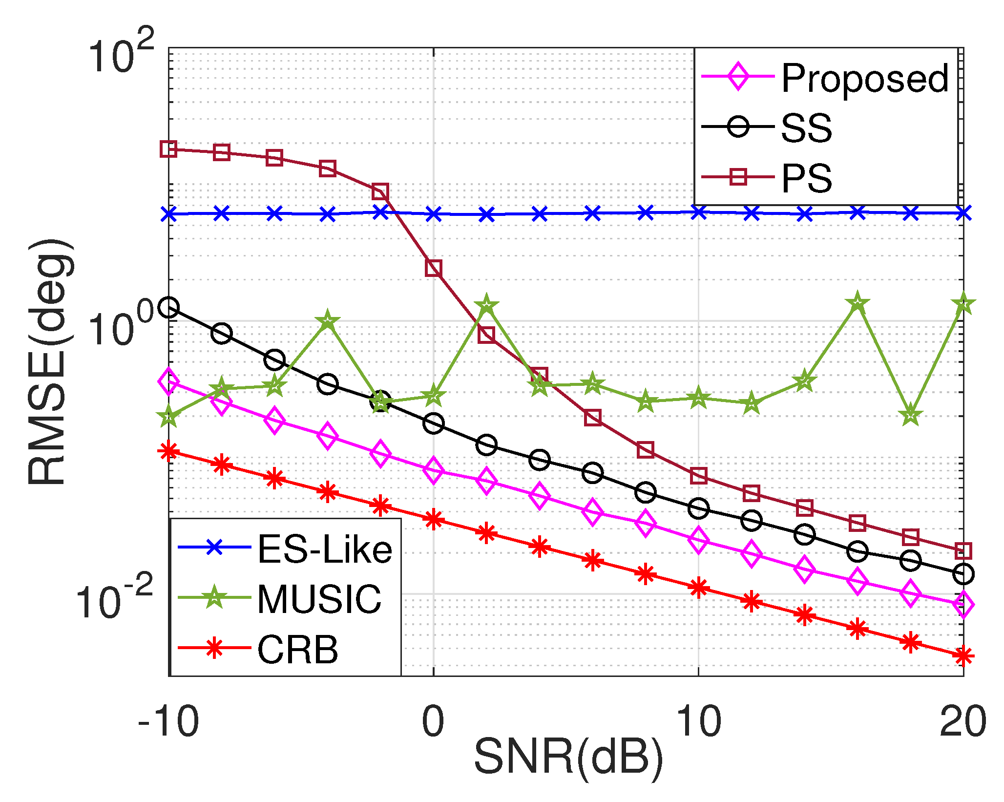
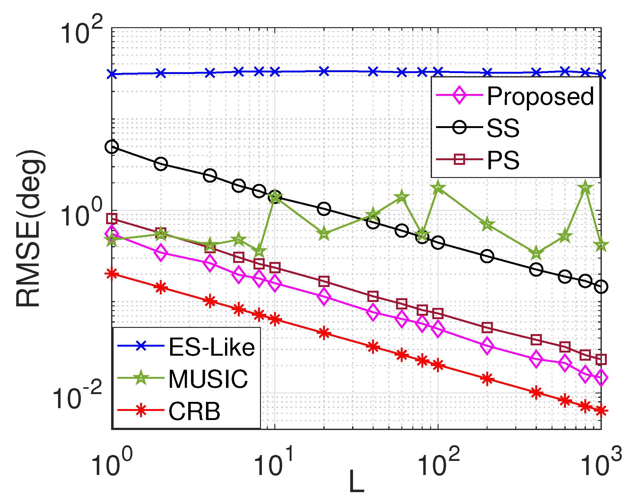
5. Simulation Results

In the simulation, we consider $K=3$ TEM sources impinging on a URA with M rows and N columns, where the inter-element spacing is d and L snapshots are collected. The signal-to-noise ratio (SNR) is defined as $\mathrm{SNR}=10lg\left({∥\mathit{Y}-{\mathit{N}}_{\mathit{Y}}∥}^2/\phantom{{∥\mathit{Y}-{\mathit{N}}_{\mathit{Y}}∥}^2{∥\mathit{N}∥}^2}{∥{\mathit{N}}_{\mathit{Y}}∥}^2\right)$, where $\mathit{Y}$ and ${\mathit{N}}_{\mathit{Y}}$ are matrices in (1). Suppose that $\theta =\left({40}^{\circ },{10}^{\circ },{60}^{\circ }\right)$, $\varphi =\left(-{15}^{\circ },{45}^{\circ },{20}^{\circ }\right)$, $\gamma =\left({12}^{\circ },{39}^{\circ },{63}^{\circ }\right)$, $\eta =\left({33}^{\circ },{47}^{\circ },-{21}^{\circ }\right)$. The source signals are modeled as autoregression (AR) processes with correlated coefficient $\alpha$. As the correlation coefficient $\alpha$ increases, the correlation of the signal gradually becomes stronger. When $\alpha =1$, the signal becomes a fully coherent signal. This article uses the magnitude of the correlation coefficient to correspond to the degree of signal correlation in multipath effects. The average root mean square error (RMSE) on 2D-DOA estimation is adopted for performance assessment.

Example 1.

Figure 3 displays the scattering result of the proposed algorithm. In Figure 3a, we set $M=6$, $N=6$, $SNR=28dB$, $L=1$, $d=2.5\lambda$, $\alpha =1$. All parameters are correctly estimated and automatically paired, indicating the suitability of the proposed algorithm for coherent sources with a single snapshot scenario. In Figure 3b where $M=6$, $N=6$, $SNR=0dB$, $L=300$, $d=2.5\lambda$, $\alpha =1$, all parameters are correctly estimated and automatically paired, demonstrating the proposed algorithm’s robustness to noise. Notably, the proposed algorithm can handle array spacing beyond the traditional half-wavelength, providing a reference for the application of sparse arrays.

Example 2.

Figure 4 shows the curve of the average RMSE of the proposed algorithm versus SNR, where $M=6$, $N=6$, $L=500$, $d=0.5\lambda$, $\alpha =1$. To enable a comprehensive comparison, we have included RMSE curves for ESPRIT-Like, SS, PS, MUSIC and the Cramer–Rao bound (CRB) in our analysis. It is readily apparent that the RMSE of all the algorithms, except for ESPRIT and MUSIC, exhibit improvement as the SNR increases. Notably, our proposed algorithm outperforms all the compared algorithms by a significant margin, which means that even when the signal propagates through a multipath channel environment and reaches the receiving array, containing a significant amount of noise due to various influences, the proposed algorithm can still provide excellent 2D-DOA estimation performance.

Example 3.

Figure 5 illustrates the comparison of average RMSE versus L, where $M=6$, $N=6$, $SNR=18dB$, $d=0.5\lambda$, $\alpha =1$. It can be observed that the RMSE gradually decreases as L increases for all the algorithms. Similar to the observation in Figure 4, the proposed algorithm provides the best RMSE performance over the entire L regions.

Example 4.

Figure 6 displays the average RMSE comparison versus α, where $M=6$, $N=6$, $SNR=2dB$, $L=500$, $d=0.5\lambda$. An intriguing finding from our analysis is that ESPRIT delivers the most favorable RMSE performance when $\alpha <0.1$ since sources in such conditions can be interpreted as non-coherent. In contrast, both SS and our proposed approach exhibit insensitivity to α, which indicates that correlated or fully coherent signals present in a multipath environment can provide stable 2D-DOA estimation. Furthermore, our proposed algorithm consistently delivers a superior RMSE compared to SS, PS and MUSIC.

Example 5.

Figure 7 displays the average RMSE comparison versus $dy$, where $M=6$, $N=6$, $SNR=18dB$, $L=500$, $\alpha =1$. As the distance between the array elements parallel to the y-axis increases, the effective aperture of the array expands, leading to a gradual improvement in DOA estimation accuracy. However, it is worth noting that the PS algorithm tends to smooth out the polarization domain information. Consequently, when the distance becomes too large, this method may yield ambiguous solutions and even lead to estimation failure. In contrast, both the SS and our proposed algorithm align with theoretical expectations. Most notably, our proposed approach provides the best estimation performance by fully utilizing both the spatial and polarization domain information available.

Example 6.

Figure 8 displays the average RMSE comparison versus N, where $M=5$, $SNR=20dB$, $L=300$, $d=0.5\lambda$, $\alpha =1$. Expanding the number of elements in an array enhances its effective aperture, resulting in improved accuracy in DOA estimation. Figure 8 provides compelling evidence that the PS algorithm is constrained by the symmetry of the array structure and only produces accurate estimates when M = N. In contrast, both the PS and our proposed algorithms exhibit similar trends, with RMSE progressively decreasing across the entire range of N. However, even in this scenario, our proposed approach outperforms all the compared algorithms. These findings suggest that our proposed algorithm has the potential to be applied to a broad range of array configurations, leading to enhanced performance in diverse applications.

6. Conclusions

In this paper, we have accomplished a matrix arrangement approach for 2D-DOA estimation of coherent sources using EMVS arrays. Unlike the exiting smoothing-based methods, the matrix rearrangement strategy is adopted to resolve the rank deficient issue. Based on numerical simulation results, it can be seen that the algorithm proposed in this paper can effectively distinguish partially correlated and fully coherent sources generated by phenomena such as reflection, scattering and diffraction in multipath channel environments. The 2D-DOA and polarization parameters are obtained via combining the normalized VCP technique with the LS technique. The proposed approach is suitable for a single snapshot scenario and scenarios where the array element spacing is greater than half a wavelength and it offers more accurate 2D-DOA estimation than the existing methods. In addition, utilizing polarization information in 2D-DOA estimation can provide a performance advantage over conventional methods that do not take polarization into account. By measuring the polarization properties of the incoming signals, it is possible to estimate the DOA of the source with higher accuracy and resolution than traditional methods, especially when the DOA is almost identical. We acknowledge the limitations of our research, which was purely theoretical in nature due to the lack of available experimental conditions. However, we remain optimistic about the potential for future experimental verification once appropriate conditions become available. We believe that such verification will provide valuable insights and further enhance the understanding of the topic.

References

1. Yu, J.; Li, J.; Sun, B.; Jiang, Y.; Xu, L. Multiple RFI sources location method combining two-dimensional ESPRIT DOA estimation and particle swarm optimization for spaceborne SAR. Remote Sens. 2021, 13, 1207. [Google Scholar] [CrossRef]
2. Luo, J.; Zhang, Y.; Yang, J.; Zhang, D.; Zhang, Y.; Zhang, Y.; Huang, Y.; Jakobsson, A. Online sparse DOA estimation based on sub–aperture recursive LASSO for TDM–MIMO radar. Remote Sens. 2022, 14, 2133. [Google Scholar] [CrossRef]
3. Wan, B.; Wu, X.; Yue, X.; Zhang, L.; Wang, L. Calibration of phased-array high-frequency radar on an anchored floating platform. Remote Sens. 2022, 14, 2174. [Google Scholar] [CrossRef]
4. Ding, X.; Hu, Y.; Liu, C.; Wan, Q. Coherent targets parameter estimation for EVS-MIMO radar. Remote Sens. 2022, 14, 4331. [Google Scholar] [CrossRef]
5. Mao, Z.; Liu, S.; Qin, S.; Haung, Y. Cramér-Rao Bound of joint DOA-range estimation for coprime frequency diverse arrays. Remote Sens. 2022, 14, 583. [Google Scholar] [CrossRef]
6. McCloud, M.J.; Scharf, L.L. A new subspace identification algorithm for high-resolution DOA estimation. IEEE Trans. Antennas Propag. 2002, 50, 1382–1390. [Google Scholar] [CrossRef]
7. Han, F.M.; Zhang, X.D. An ESPRIT-Like algorithm for coherent DOA estimation. IEEE Antennas Wireless Propag. Lett. 2005, 4, 443–446. [Google Scholar] [CrossRef]
8. Shen, Q.; Liu, W.; Cui, W.; Wu, S.L. Underdetermined DOA Estimation Under the Compressive Sensing Framework: A Review. IEEE Access 2016, 4, 8865–8878. [Google Scholar] [CrossRef]
9. Zhang, Y.; Ng, B.P. MUSIC-like DOA estimation without estimating the number of sources. IEEE Trans. Signal Process. 2010, 58, 1668–1676. [Google Scholar] [CrossRef]
10. Wu, Y.; Liao, G.; So, H.C. A fast algorithm for 2-D direction-of-arrival estimation. Signal Process. 2003, 83, 1827–1831. [Google Scholar] [CrossRef] [Green Version]
11. Xi, N.; Li, P.L. A computationally efficient subspace algorithm for 2-D DOA estimation with L-shaped array. IEEE Signal Process. Lett. 2014, 21, 971–974. [Google Scholar] [CrossRef]
12. Chen, F.J.; Kwong, S.; Kok, C.W. ESPRIT-Like two-dimensional DOA estimation for coherent signals. IEEE Trans. Aerosp. Electron. Syst. 2010, 46, 1477–1484. [Google Scholar] [CrossRef]
13. Wen, F.Q.; Shi, J.P.; Gui, G.; Gacanin, H.; Dobre, O.A. 3-D Positioning Method for Anonymous UAV Based on Bistatic Polarized MIMO Radar. IEEE Internet Things J. 2023, 10, 815–827. [Google Scholar] [CrossRef]
14. Zhang, B.; Xu, G.; Zhou, R.; Zhang, H.; Hong, W. Multi-channel back-projection algorithm for mmwave automotive MIMO SAR imaging with Doppler-division multiplexing. IEEE J. Sel. Top. Signal Process. 2022, 17, 445–457. [Google Scholar] [CrossRef]
15. Xu, G.; Zhang, B.J.; Yu, H.W.; Chen, J.; Xing, M.; Hong, W. Sparse Synthetic Aperture Radar Imaging from Compressed Sensing and Machine Learning: Theories, Applications and Trends. IEEE Geosci. Remote. Sens. Mag. 2022, 10, 32–69. [Google Scholar] [CrossRef]
16. Xu, G.; Zhang, B.J.; Chen, J.L.; Hong, W. Structured Low-Rank and Sparse Method for ISAR Imaging With 2-D Compressive Sampling. IEEE Trans. Geosci. Remote. Sens. 2022, 60, 5239014. [Google Scholar] [CrossRef]
17. Wen, F.Q.; Guan, G.; Gacanin, H.; Sari, H. Compressive Sampling Framework for 2D-DOA and Polarization Estimation in mmWave Polarized Massive MIMO Systems. IEEE Trans. Wirel. Commun. 2022, 22, 3071–3083. [Google Scholar] [CrossRef]
18. Wong, K.T.; Zoltowski, M.D. Closed-form direction finding and polarization estimation with arbitrarily spaced electromagnetic vector-sensors at unknown locations. IEEE Trans. Antenna. Propag. 2000, 48, 671–681. [Google Scholar] [CrossRef] [Green Version]
19. Zhang, D.; Zhang, Y.; Zheng, G. ESPRIT-Like two-dimensional DOA estimation for monostatic MIMO radar with electromagnetic vector received sensors under the condition of gain and phase uncertainties and mutual coupling. Sensors 2017, 17, 2457. [Google Scholar] [CrossRef] [Green Version]
20. Ahmed, T.; Zhang, X.; Zheng, W. DOA estimation for coprime EMVS arrays via minimum distance criterion based on PARAFAC analysis. IET Radar Sonar Nav. 2019, 13, 65–73. [Google Scholar] [CrossRef]
21. Zhang, L.; Wang, H.; Wen, F.Q.; Shi, J.P. PARAFAC estimators for coherent targets in EMVS-MIMO radar with arbitrary geometry. Remote Sens. 2022, 14, 2905. [Google Scholar] [CrossRef]
22. Fu, M.C.; Zheng, Z.; Wang, W.Q.; So, H.C. Coarray Interpolation for DOA Estimation Using Coprime EMVS Array. IEEE Signal Process. Lett. 2021, 28, 548–552. [Google Scholar] [CrossRef]
23. Lan, X.; Liu, W.; Ngan, H.Y. Joint DOA and Polarization Estimation With Crossed-Dipole and Tripole Sensor Arrays. IEEE Trans. Aerosp. Electron. Syst. 2020, 56, 4965–4973. [Google Scholar] [CrossRef]
24. Rahamim, D.; Tabrikian, J.; Shavit, R. Source localization using vector sensor array in a multipath environment. IEEE Trans. Signal Process. 2004, 52, 3096–3103. [Google Scholar] [CrossRef]
25. Rahamim, D.; Shavit, R.; Tabrikian, J. Coherent source localization using vector sensor arrays. In Proceedings of the 2003 IEEE International Conference on Acoustics, Speech and Signal Processing, ICASSP ’03, Hong Kong, China, 6–10 April 2003; Volume 5, pp. V–141. [Google Scholar] [CrossRef]
26. He, J.; Jiang, S.L.; Wang, J.T.; Liu, Z. Polarization difference smoothing for direction finding of coherent signals. IEEE Trans. Aerosp. Electron. Syst. 2010, 46, 469–480. [Google Scholar] [CrossRef]
27. Wu, J.L.; Wen, F.Q.; Shi, J.P. Fast angle estimation in MIMO system with direction-dependent mutual coupling. IEEE Commun. Lett. 2021, 25, 2913–2917. [Google Scholar] [CrossRef]
28. Ren, S.W.; Ma, X.C.; Yan, S.F.; Hao, C.P. 2-D unitary ESPRIT-Like direction-of-arrival (DOA) estimation for coherent signals with a uniform rectangular array. Sensors 2013, 13, 4272–4288. [Google Scholar] [CrossRef] [Green Version]
29. Cao, M.Y.; Mao, X.P.; Long, X.Z.; Huang, L. Tensor approach to DOA estimation of coherent signals with electromagnetic vector-sensor array. Sensors 2018, 18, 4320. [Google Scholar] [CrossRef] [Green Version]
30. Wong, K.T.; Yuan, X. Vector Cross-Product Direction-Finding with an Electromagnetic Vector-Sensor of Six Orthogonally Oriented But Spatially Noncollocating Dipoles/Loops. IEEE Trans. Signal Process. 2010, 59, 160–171. [Google Scholar] [CrossRef]
31. Wong, K.T.; Zoltowski, M.D. High accuracy 2D angle estimation with extended aperture vector sensor arrays. In Proceedings of the 1996 IEEE International Conference on Acoustics, Speech and Signal Processing Conference Proceedings, Atlanta, GA, USA, 9 May 1996; Volume 5, pp. 2789–2792. [Google Scholar] [CrossRef]
32. Wen, F.Q.; Ren, D.; Zhang, X.X.; Gui, G.; Adebisi, B.; Sari, H.; Adachi, F. Fast localizing for anonymous UAVs oriented toward polarized massive MIMO systems. IEEE Internet Things J. 2023. [Google Scholar] [CrossRef]
33. Zheng, Z.; Zheng, Y.; Wang, W.Q.; Zhang, H.B. Covariance matrix reconstruction with interference steering vector and power estimation for robust adaptive beamforming. IEEE Trans. Veh. Technol. 2018, 67, 8495–8503. [Google Scholar] [CrossRef]
Figure 1. Illustration of the polarized URA.
Remotesensing 15 03308 g001
Figure 2. Normalized dot product versus DOA separation.
Remotesensing 15 03308 g002
Figure 3. Scattering results of the proposed approach: (a) 2D-DOA estimation with a single snapshot (b) 2D-DOA estimation with multiple snapshots.
Remotesensing 15 03308 g003
Figure 4. Average RMSE vs. SNR in the second example.
Remotesensing 15 03308 g004
Figure 5. Average RMSE versus L in the third example.
Remotesensing 15 03308 g005
Figure 6. Average RMSE versus α in the fourth example.
Remotesensing 15 03308 g006
Figure 7. Average RMSE versus d y in the fifth example.
Remotesensing 15 03308 g007
Figure 8. Average RMSE versus N in the sixth example.
Remotesensing 15 03308 g008