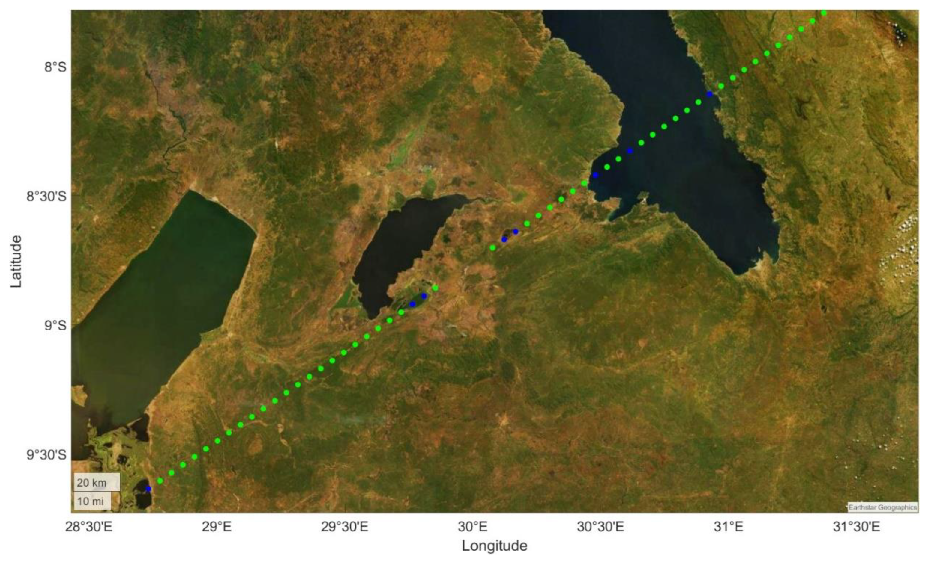
Abstract
Inland water bodies, wetlands and their dynamics have a key role in a variety of scientific, economic, and social applications. They are significant in identifying climate change, water resource management, agricultural productivity, and the modeling of land–atmosphere exchange. Changes in the extent and position of water bodies are crucial to the ecosystems. Mapping water bodies at a global scale is a challenging task due to the global variety of terrains and water surface. However, the sensitivity of spaceborne Global Navigation Satellite System Reflectometry (GNSS-R) to different land surface properties offers the potential to detect and monitor inland water bodies. The extensive dataset available in the Cyclone Global Navigation Satellite System (CYGNSS), launched in December 2016, is used in our investigation. Although the main mission of CYGNSS was to measure the ocean wind speed in hurricanes and tropical cyclones, we show its capability of detecting and mapping inland water bodies. Both bistatic radar cross section (BRCS) and signal-to-noise ratio (SNR) can be used to detect, identify, and map the changes in the position and extent of inland waterbodies. We exploit the potential of unsupervised machine learning algorithms, more specifically the clustering methods, K-Means, Agglomerative, and Density-based Spatial Clustering of Applications with Noise (DBSCAN), for the detection of inland waterbodies. The results are evaluated based on the Copernicus land cover classification gridded maps, at 300 m spatial resolution. The outcomes demonstrate that CYGNSS data can identify and monitor inland waterbodies and their tributaries at high temporal resolution. K-Means has the highest Accuracy (93.5%) compared to the DBSCAN (90.3%) and Agglomerative (91.6%) methods. However, the DBSCAN method has the highest Recall (83.1%) as compared to Agglomerative (82.7%) and K-Means (79.2%). The current study offers valuable insights and analysis for further investigations in the field of GNSS-R and machine learning.
1. Introduction
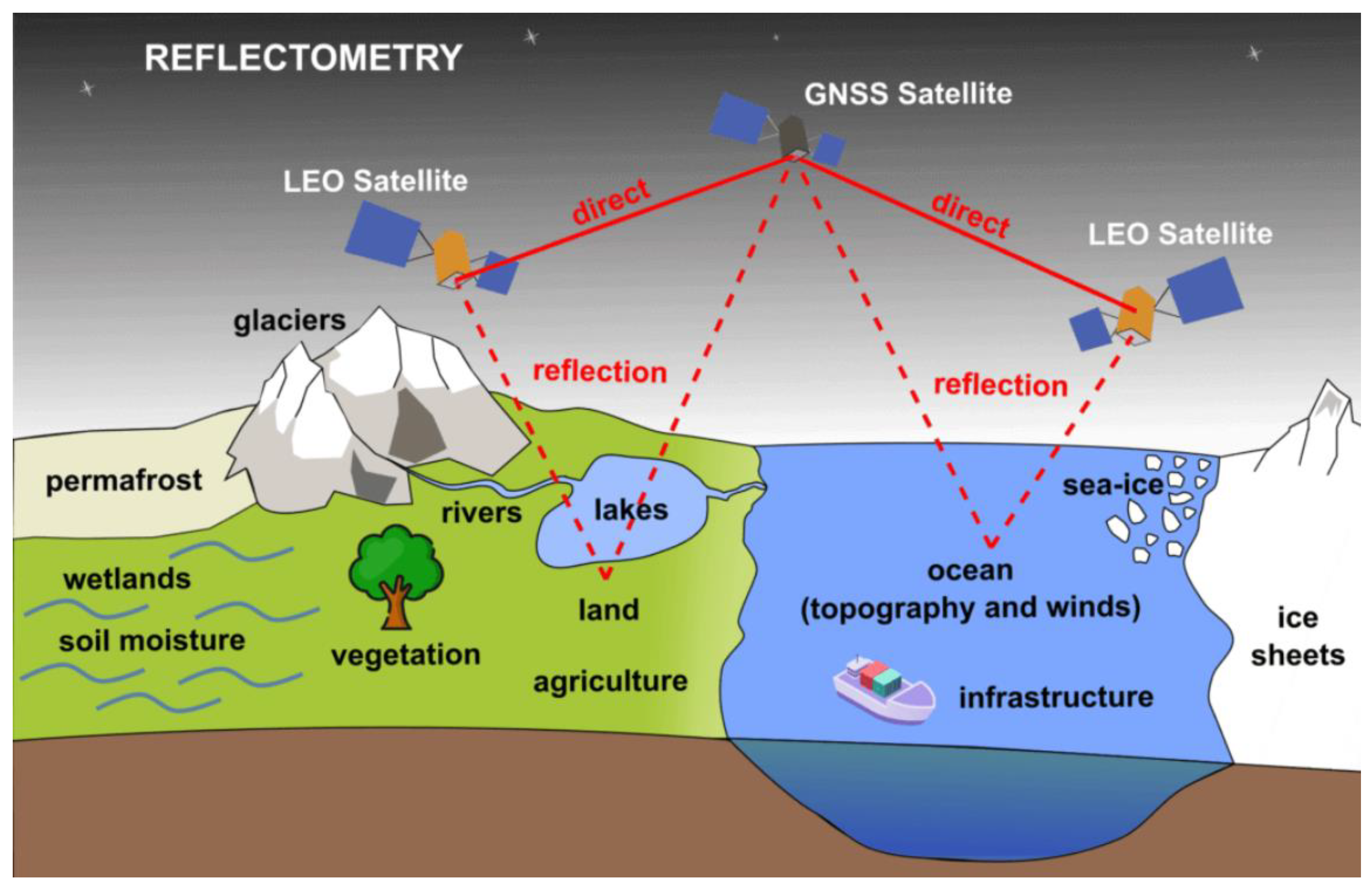
Natural disasters, such as hurricanes, floods, ocean currents, volcanic eruptions, and solar variations cause many serious disturbances to the environment. Economic losses due to such catastrophic events have increased significantly around the world [1]. Therefore, one of the vital tasks of Earth science is the observation, analysis and prediction of climate change and weather processes endangering the planet. Nowadays, the great number of satellites in combination with the huge quantity of receivers in regional and global ground networks provide substantial scientific data records. These data are analyzed and finally used in geophysical models to characterize the Earth system. Airborne observations and land surveying are the traditional methods used for the observation of natural disasters. However, disasters mostly happen on a large scale and these methods are either impossible to be implemented or costly and slow [2]. Thus, space-based remote sensing (RS) could be considered an innovative technique that provides up-to-date data from various sensors. Realizing the full potential of all-weather L-band signals, many other applications, including GNSS-RS, have been introduced in recent decades. The innovative Global Navigation Satellite System Reflectometry (GNSS-R) technique, that uses GNSS signals reflected off the Earth’s surface, as it can be seen in Figure 1, has garnered widespread interest for Earth observation [3,4].

Figure 1.
GNSS Reflectometry using receivers on satellites (image credit: GGOS, https://ggos.org/item/gnss-reflectometry/, accessed on 21 May 2023).
Detection of inland water bodies is important for several applications, including water resource management [5], assessment of climate change along with the development of mitigation techniques [6,7], agricultural productivity [8], and the modeling of exchange between land and atmosphere [9]. Moreover, accurate knowledge of inland water is key to the operational aspects of RS missions, such as Soil Moisture and Ocean Salinity (SMOS) and Soil Moisture Active Passive (SMAP) missions [10,11]. The sensitivity of spaceborne GNSS-R to various land surface properties offers the potential for dynamic inland water body monitoring.
Monitoring inland water bodies and their dynamics using GNSS-R measurements is one of the latest promising applications. Measurements carried out via GNSS-R missions have shown stronger reflected power over inland waters, that has been attributed to coherent specular scattering than the diffuse scattering coming from the surrounding land [12]. In the last decade, the ability of GNSS-R to observe the global surface water distribution by generating maps of inland water bodies and other inundated areas has been demonstrated. TechDemoSat-1 (TDS-1), launched in 2014, fully demonstrated the sensitivity of GNSS-R to temporal changes over inland water bodies [13,14]. Cyclone Global Navigation Satellite System (CYGNSS) consists of eight microsatellites in the inclined orbits launched in December 2016 [15,16]. Furthermore, upcoming GNSS-R missions and further ideas are being developed [17,18,19,20].
Several previous studies have attempted to develop coherence-detection algorithms. Many of the methods rely on mean values within the Delay Doppler Map (DDM) average region within varying Delay Doppler extents [21,22], SNRs [23], the DDM trailing edge slope [24], or a combination of these DDM quantities. Moreover, an image processing algorithm is presented by [25], that leverages the surface reflectivity signal to create a mask of inland waterbodies at 0.01° × 0.01° spatial resolution, using one month of data due to CYGNSS’ short return time. Signal-to-noise ratio (SNR) values are being transformed into a map of standard deviation values. Then, they map water and dry land using segmentation function. Comparing with MODIS [26], they show that most of the smaller tributaries identified via their algorithm are missing in the MODIS mask. They also used data taken over the Congo Basin in a period which coincides with the current study. However, they used statistics and segmentation methods instead of the traditional unsupervised machine learning algorithms. Moreover, during the same year, it was demonstrated that CYGNSS data present high reflectivity in both inland waters and wetlands covered by vegetation canopies [27]. Thus, CYGNSS data are capable of detecting and mapping both inland water bodies and wetlands, and floods. The main parameter used by [28] for the detection of inundated areas was the DDM SNR, retrieved from the L1 data product. Initially, a data preparation procedure was applied to remove outliers and discard low-quality data. After that, SNR measurements were interpolated to a regular grid over the study area. A threshold was used to distinguish the inundated from non-inundated areas. However, this threshold was used for the detection of inundation in this study and cannot generally be used for the detection of floods.
Moreover, a machine learning method for the detection of inland waterbodies using CYGNSS data is implemented via the random under sampling boosted (RUS Boost) algorithm [29]. As a supervised classification problem, the high-resolution Global Surface Water (GSW) data (30 m × 30 m) were used for the labeling and evaluation. The CYGNSS data are gridded into 0.01° × 0.01° cells. For Congo and Amazon basins, the classifier has a 3.9% and 14.2% higher water detection accuracy, respectively. The classifier was trained and tested with data over the Congo basin but the results over the Amazon basin indicate that the proposed technique is more general compared to the water mask technique. Finally, in [30] the authors proposed a method related to the extent of power spread across the DDM to flag coherency. The detector compares the power concentrated within the ±1 Delay bins and ±2 Doppler bin region about the specular bin with the total power outside this region. The results show that the coherence is primarily associated with inland water bodies. Therefore, the detector develops the creation of dynamic inland water body masks at spatial resolutions ranging from 1 to 3 km. Comparisons against Pekel water masks indicate that the accuracy of detecting water bodies is higher than 80% [31].
The key contribution of this current study is the exploitation of the unsupervised Machine Learning algorithms’ problems, more specifically clustering methods, such as K-Means, Agglomerative, and Density-based Spatial Clustering of Applications with Noise (DBSCAN) for the detection of inland water bodies. K-Means method has the highest Accuracy, against the Agglomerative and DBSCAN methods. These methods also show their ability to detect small tributaries, that are missing from the Copernicus land cover classification gridded maps at 300 m spatial resolution produced in the context of the Copernicus Climate Change Service (C3S). Moreover, both BRCS and SNR observations can be employed to make maps on short timescales using weekly, monthly, or seasonal data, in contrast to low temporal resolution water masks of MODIS and Copernicus, taking advantage of the mean revisit time of CYGNSS observations (7 h). However, the algorithms implemented in the current study are traditional clustering methods forming baseline scenario for alternative and novel data-scientific approaches. Therefore, further research could also be performed using unsupervised or supervised artificial neural networks for the detection and mapping of inland waterbodies.
2. Dataset
2.1. CYGNSS Mission
CYGNSS is the first mission fully dedicated to GNSS-R conducted by the National Aeronautics and Space Administration (NASA). The micro-satellites dispersed over a 510 km circular orbit at a 35° inclination angle, each capable of measuring four simultaneous reflections, i.e., 32 spatially separated measurements every second in total. The parameters of CYGNSS satellites are presented in Table 1. Also, the mission provides nearly gap-free Earth coverage with a median revisit time of 2.8 h and a mean revisit time of 7.2 h [16]. CYGNSS addresses the shortcomings by exploiting all-weather GPS signals. GPS satellites operate at a frequency of 1.575 GHz (L-band), allowing measurements within the eyewall of hurricanes, cloud, and rain with no significant degradation as well as observations of the surface under canopies [27,32]. Optimized to estimate wind speed over oceans, CYGNSS also showed its capability to sense standing water over land [33] and soil moisture [33,34]. It offers a wide variety of applications.

Table 1.
The CYGNSS satellite parameters. The referred spatial resolution is the nominal.
2.2. CYGNSS Data—Delay Doppler Map (DDM)
The CYGNSS data was retrieved via the FTP server from the NASA Earth Observing System Data and Information System (EOSDIS) data center, called Physical Oceanography Distributed Active Archive Center (PO. DAAC). In this study, Level 1 (L1) version 3.0 product is used, which contains geo-located Delay Doppler Maps (DDMs) and the extracted Bistatic Radar Cross Section (BRCS). Other useful scientific and engineering measurement parameters include the DDM of Normalized Bistatic Radar Cross Section (NBRCS), the Delay Doppler Map Average (DDMA), the Leading-Edge Slope (LES) of the integrated delay waveform and the DDM signal-to-noise ratio (SNR) expressed in dB. The primary output of CYGNSS is the 17-delay- and 11-Doppler-bins DDMs, where delay and Doppler bin resolutions are 249.4 ns and 500 Hz, respectively. The surface properties, as one of the parameters affecting DDMs, change the pattern of scattered signals and eventually, it will change the statistical characteristics and histogram of a DDM.
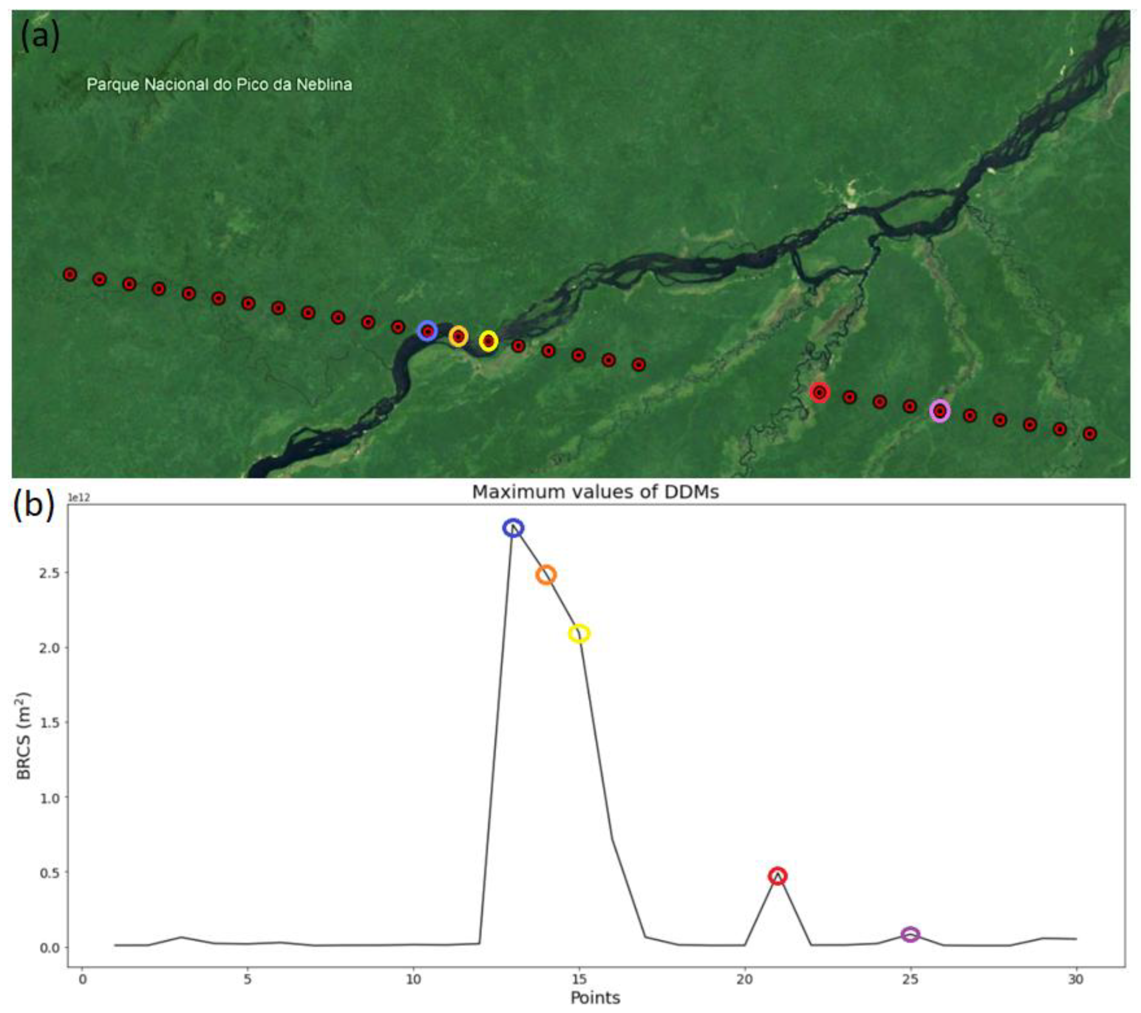
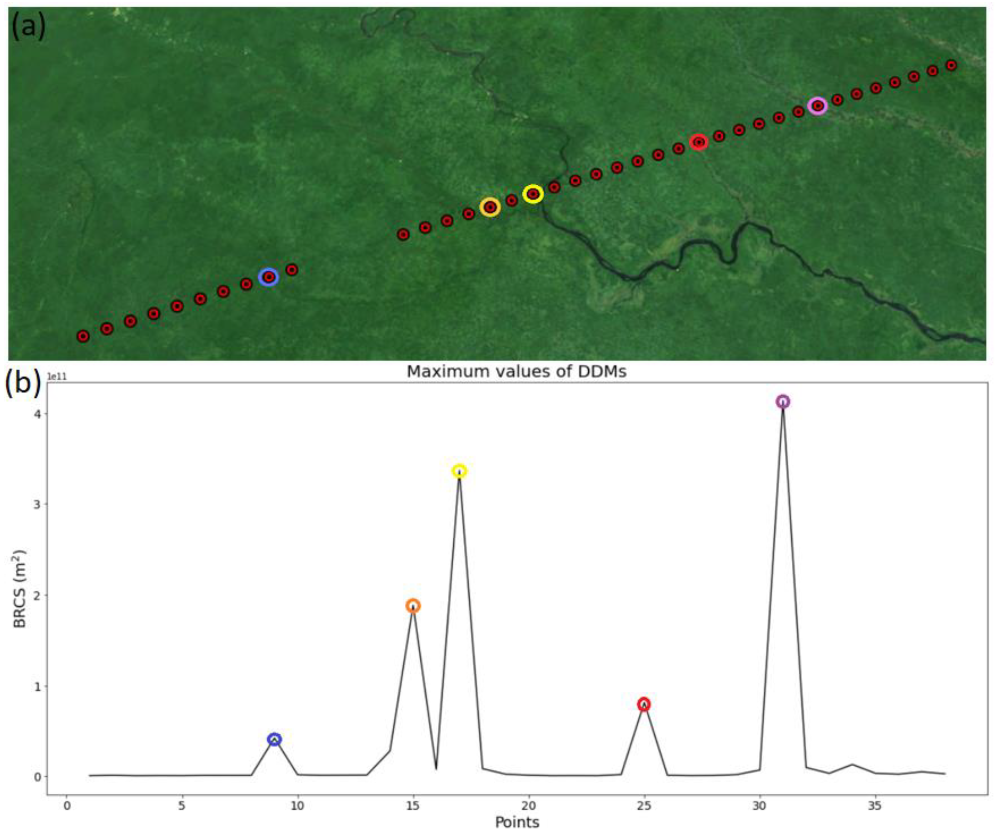
Rivers and lakes lead reflect the signals coherently with a power substantially stronger than that of the diffuse scattering. The strong coherent scattering over inland waterbodies can be illustrated using CYGNSS reflection track that passes over a variety of terrain conditions. Over land, the along-track resolution is approximately 7 km (3.5 km since July 2019) and the footprint cross track is between 0.5 and 1 km depending on the incidence angle, the reflection geometry, the surface state and roughness [25]. The tracks of the specular points over the river Rio Negro [0°S–65°W] and river Rio Uapes [1°N–68°W], tributaries of Amazon River, are shown in Figure 2 and Figure 3, respectively.

Figure 2.
(a) Track over river Rio Negro and (b) the maximum values of DDMs bin BRCS of the track.
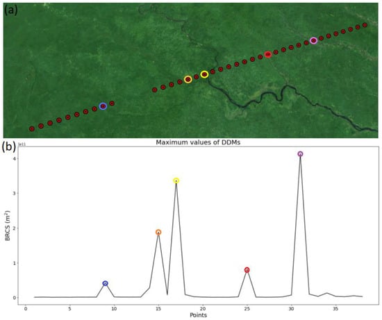
Figure 3.
(a) Track over river Rio Uapes and (b) the maximum values of DDMs bin BRCS of the track.
The maximum values correspond to the greatest strength of reflected signals of each DDM along-track, which occur normally at specular points. As it can be seen, the strength of coherent scattering signal over river (blue, orange, and yellow circles) is extremely higher (>2 × 10¹² m2) than the reflected signal over land (~109 m2). Also, the strength of the scattered signal over the red specular point (~5 × 10¹¹ m2) is of high power, since the signal reflects off from vegetated wetlands—close enough to small tributary of river—showing strong coherent features. The same phenomenon occurs both over purple specular point area and over the last two specular points.
Furthermore, the strong coherent scattering signals over inland waterbodies are also depicted along-track over river Rio Uapes. Although the width of the main river is less than 700 m, reflected signals show strong coherent features. Except for the blue specular point, all specular points are exactly located over inland waterbodies. As it can be seen in Figure 3, over inland water bodies the BRCS maximum values from DDMs BRCS are between 1 × 10¹¹ m2 and 4.5 × 10¹¹ m2. It is worth mentioning that the width of tributaries (orange, red and purple areas) is less than 100 m. As it can be understood, the BRCS of measurement over inland waterbodies showing strong coherent features can be used for mapping inland waterbodies and wetland inundation.
2.3. CYGNSS Data—Signal-to-Noise Ratio (SNR)
Previous graphs depict the BRCS maximum values from DDMs BRCS measurements over the specular points along each track. However, the coherent scattering from the smooth surfaces of inland water bodies could be ~30 dB stronger than diffuse scattering from rough surfaces, and this demonstrated that the smooth surface extends over the complete first Fresnel zone (~0.5 × 0.5 km2) [35,36]. As it is depicted below, the signal-to-noise ratio (SNR) of the reflected signals is highly variable, affected by surface type and roughness, vegetation water content, and vegetation density.
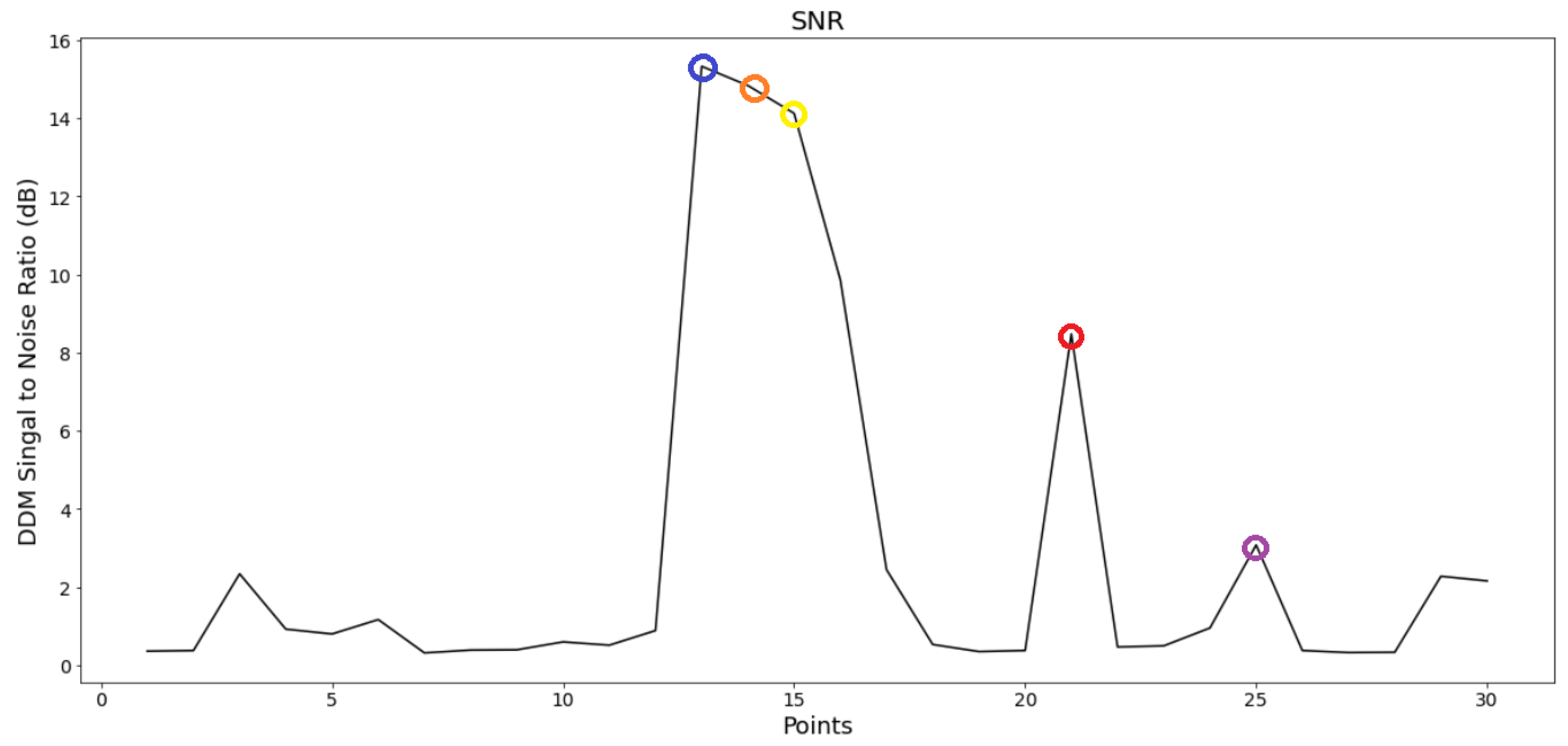
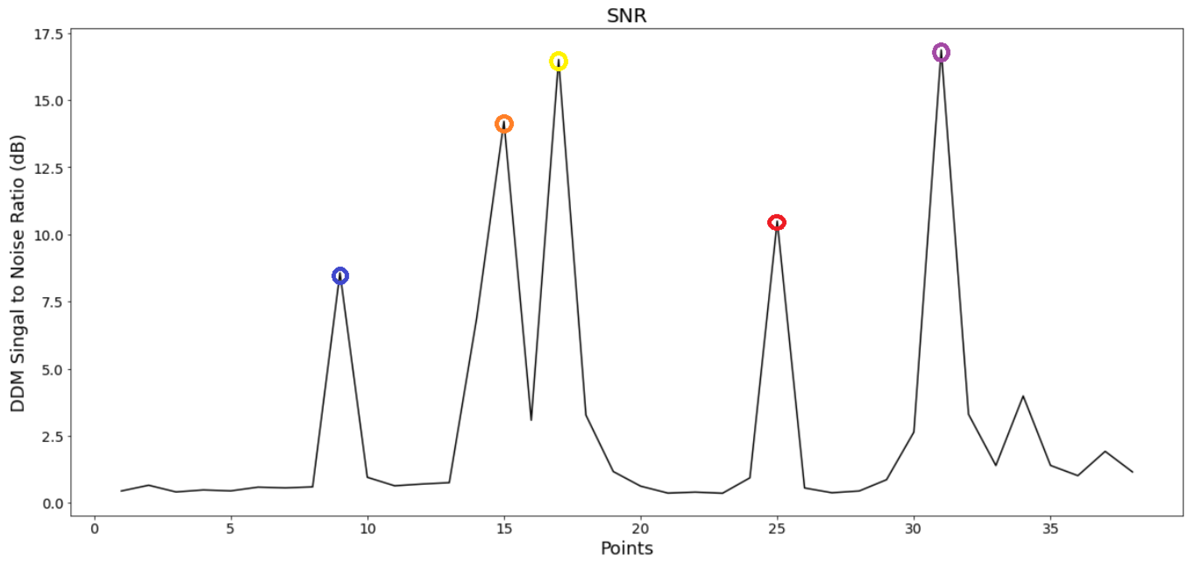
As illustrated in Figure 4 and Figure 5, the DDM SNR over a 100 m width water body is ~16 dB stronger than the that over the land surface surrounding the small water body. Figure 4 shows the SNR of the measurements over river Rio Negro, whose BRCS was given in Figure 2. Also, Figure 5 plot the SNR corresponding to the same track over river Rio Uapes shown in Figure 3 in terms of BRCS. As it is shown, the reflected signals over sparsely vegetated areas located close to the river show high signal-to-noise ratio (~9 dB).
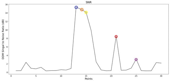
Figure 4.
DDM SNR measurements over river Rio Negro track.
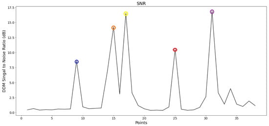
Figure 5.
DDM SNR measurements over river Rio Uapes track.
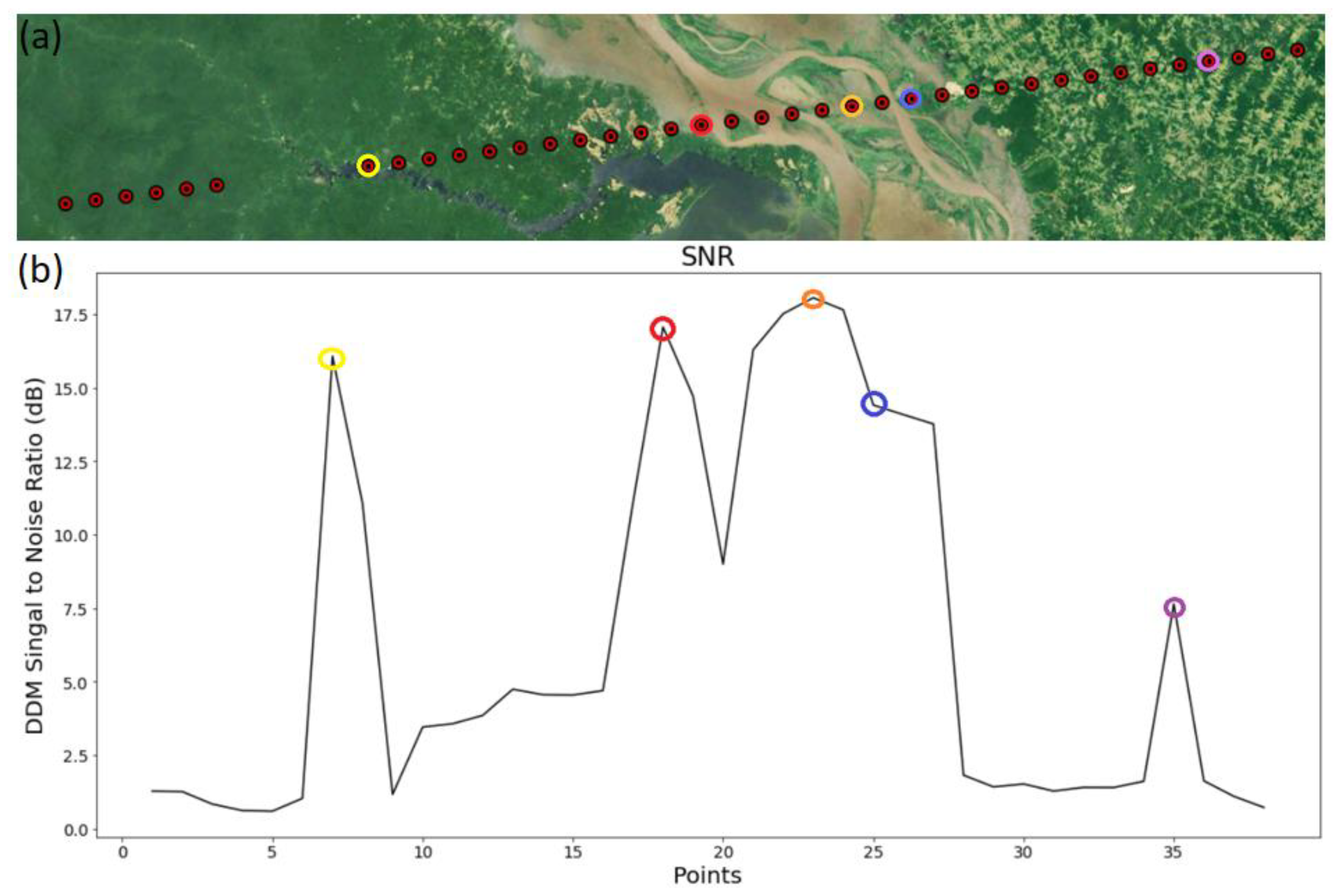
As demonstrated, SNR measurements can be used for the detection and mapping of inland waterbodies. Apart from the tributaries of the Amazon River, in Figure 6 the SNR measurements over the main part of river is shown, where the width is approximately 10 km.

Figure 6.
(a) Track over the main part of the Amazon river and (b) the DDM SNR measurements of the track.
As it is depicted, the strength of reflected signal over the yellow specular point, which is above inland waterbody is higher than 16 dB, like the power of scattered signals above the main part of river (red, orange and blue specular points). In the main part of river, the huge quantity of water covers the sparsely vegetated areas of the Amazon and as the track moves across the river. The highest SNR value is shown in orange, which is as large as ~18 dB. Signals reflected from densely vegetated wetlands, as in the purple specular point, lead to a weaker SNR (~7.5 dB). Although the purple specular point is not exactly above the tributary, SNR value shows strong specular features, and it can be used for detecting and mapping wetland inundations. Over heterogeneous areas, such as in the track depicted below, the signal over specular points can be partly reflected from the water and partly from its surrounding. Additionally, we should consider that the calculated specular point location is not exactly accurate but there is an uncertainty. In [37] it is demonstrated that factors, such as the shape of the scattering surface combined with the Fresnel zone geometry, vegetation attenuation, and surface roughness can complicate retrievals.
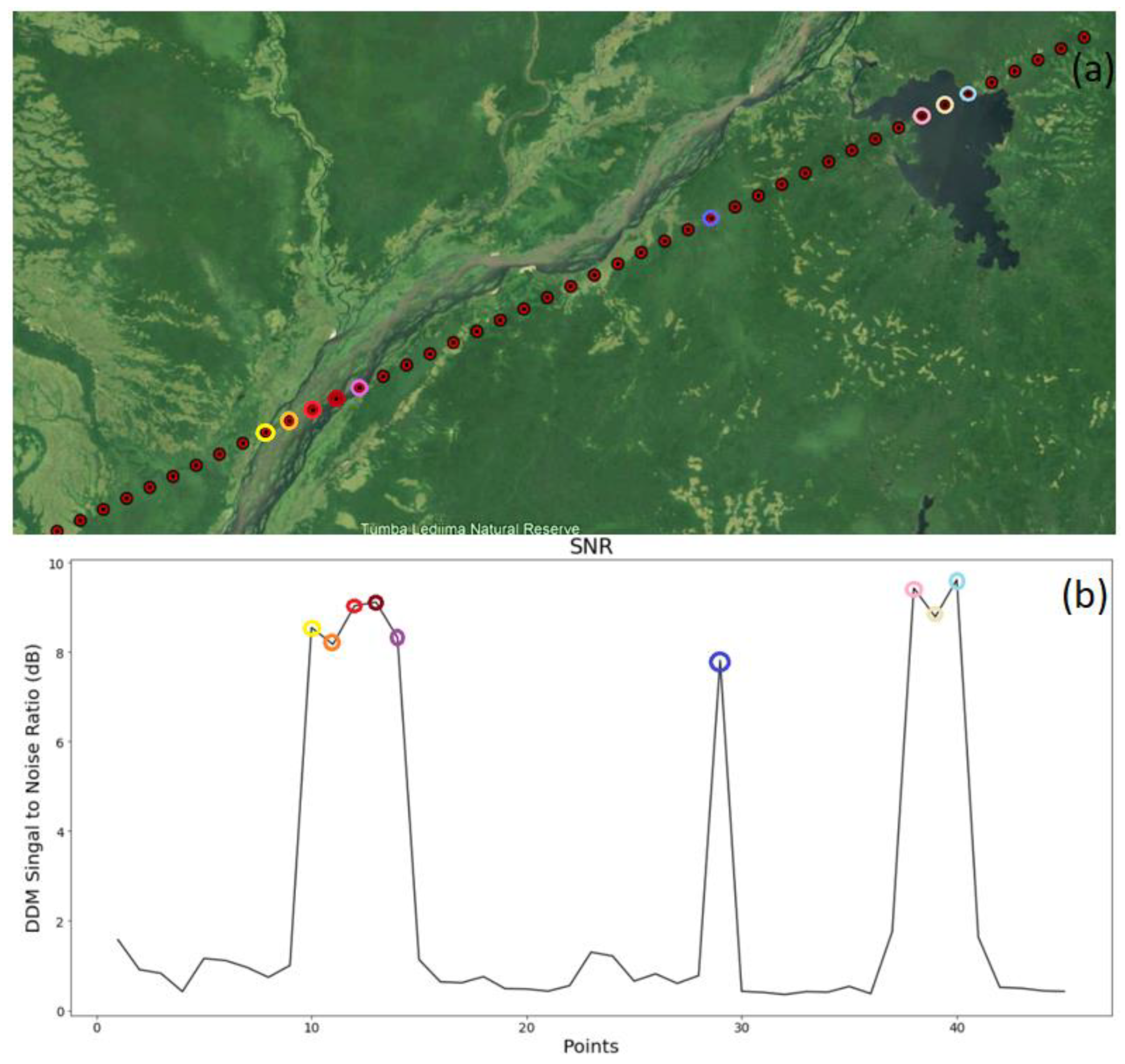
Figure 7 illustrates the track of specular points over the Congo River in Africa (1°S–17°E). As it can be seen, the SNR between the 10th and 14th points is approximately ~9 dB, while over Lake Tumba (38th, 39th and 40th specular points) is a few dB higher than SNR over the Congo River. The SNR of the measurement shown above in blue is approximately ~8 dB.
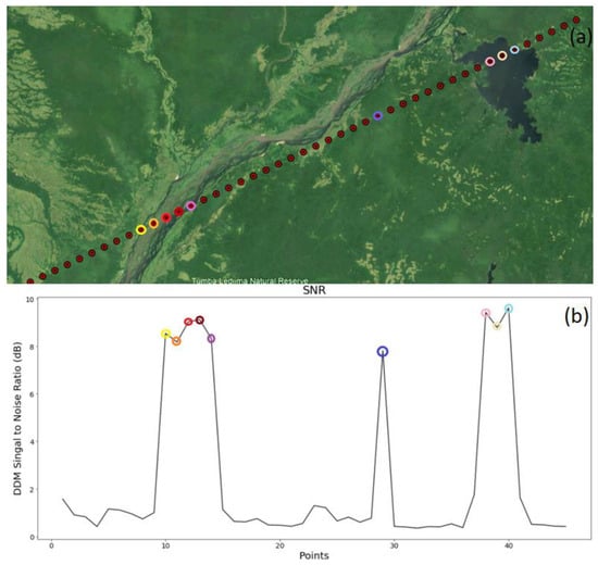
Figure 7.
(a) Track over the Congo river and (b) the DDM SNR measurements of the track.
It is noticed that scattered signals do not show so strong coherent features as in the cases of Rio Negro, Rio Uapes and the Amazon rivers (~16 dB). This should be expected as the large width of the Congo River as well as the big size of the Tumba Lake allow the formation of significant wave heights by wind that result in strong diffuse scattering.
2.4. SNR Observations Preprocessing
Prior to performing the clustering algorithms, the dataset is filtered in order to obtain both more accurate results with better quality, and to ensure that the implementation of algorithms is less time-consuming. Since the goal of current study is to classify the observations into two distinct groups (land and inland water bodies) implementing clustering algorithms, measurements over sea surface were filtered. Moreover, many ways were tested to fill the missing data through the implementation of clustering algorithms. Two of the methods used are either to just fill them up with 0 or fill them up each time with the average value of each track. Furthermore, the median of each track was used to fill incorrect data. However, implementation of the aforementioned methods in clustering algorithms resulted in several false clustered observations, and the model accuracy was significantly reduced. Thus, the best method is the complete removal of missing data. Finally, Table 2 shows the final sample size after quality-filtering of the data. The two first columns are indicative of one day measurements from one satellite (cyg2) in 2018 and 2019, while the last column reports the number of observations for one-week measurements with the contribution of all satellites. Therefore, the final sample size is taken after filtering both the observations over sea surface and the missing data.

Table 2.
Sample sizes of the data before and after filtering.
As can be seen, the number of final observations is around 25% of the initial sample, and the processing of final sample is substantially less time-consuming. Moreover, as explained above, after July 2019 the along-track resolution is 3.5 km instead of 7 km. The higher quantity of observations after July 2019 is depicted in Table 2, comparing the quantity of observations between 1 August 2018 and 1 August of 2019.
3. Methods
In recent years, machine learning methods have become ubiquitous in everyday life. These methods are also commonly used for the extraction of required geophysical information from GNSS data. The most suitable unsupervised ML method for the detection of inland waterbodies is Clustering, since it refers to a very broad set of techniques for finding subgroups, or clusters in a dataset. Clustering assigns a number to each observation, indicating in which cluster a particular observation belongs to. Thus, Clustering seeks to discover structure, meaning distinct clusters and homogeneous subgroups, among the observations [38]. The current study, for the detection of inland waterbodies, is focused on three of the best-known clustering approaches: K-Means, Agglomerative and DBSCAN, which stands for Density-based spatial clustering of applications with noise. The desired number of homogeneous subgroups in which observations should be clustered is two, since the target is the separation of land and inland waterbodies observations as described above.
3.1. K-Means Clustering
K-means is an elegant and one of the simplest and most used algorithms for partitioning a data set into K distinct, non-overlapping clusters. For the implementation of K-means clustering, the number of clusters equal to two is specified. The idea behind K-means is that a good clustering is one for which the within-cluster variation is as small as possible. The within-cluster variation for cluster Ck is a measure W (Ck) of the amount by which the observations within a cluster differ from each other. Therefore, the problem solved is:
Equation (1) interprets that the observations must be partitioned into K clusters such that the total within-cluster variation, summed over all K clusters, is as low as possible. There are many ways to define the concept of within-cluster variation, but by far the most common choice involves squared Euclidean distance and defined as:
where, |Ck| denotes the number of observations in the kth cluster. So, the within-cluster variation for the kth cluster is the sum of all the pairwise squared Euclidean distances between the observations in the kth cluster, divided by the total number of observations in the kth cluster. K-means is guaranteed to decrease the value of the objective at each step. As the algorithm is run, the clustering obtained will continuously be improved until the result no longer changes and then a local optimum is reached [38].
3.2. Agglomerative Clustering
The next method used for the detection of inland water bodies is the most common type of hierarchical clustering, called Agglomerative. It is a “bottom-up” approach since the algorithm starts by declaring each observation in its own cluster and then merges the two most similar clusters until a stopping criterion is satisfied. Using the scikit-learn library, the stopping criterion is the desired number of clusters [39]. Thus, similar clusters are merged until only two clusters are left. Afterwards, there are several methods to specify how exactly the “most similar cluster” is measured. This similarity measure is always defined between two existing clusters. In the current study, the linkage criterion used is the ‘ward’, that picks the two clusters being merged such that the variance within all clusters increases the least [40].
3.3. DBSCAN Clustering
Density-based spatial clustering of applications with noise (DBSCAN) is a well-known data clustering algorithm that is commonly used in data mining and machine learning proposed by [41]. The main benefits of DBSCAN are that it does not require to set the number of clusters a priori, in contrast with K-means and agglomerative methods, and it can capture clusters of complex shapes and identify points that does not belong to any cluster. Based on a set of data, DBSCAN groups cluster observations that are close to each other based on a distance measurement (usually Euclidean distance) and a minimum number of points. Also, it marks the points that are in low-density regions as outliers.
Furthermore, DBSCAN requires two main hyperparameters: eps and min_samples. The first one specifies how close observations should be to each other to be considered as a part of the same cluster. Thus, if the distance between two points is lower or equal to the value of eps, these points are considered neighbors. Moreover, min_samples define the minimum number of points to form a cluster. For example, if we set the parameter equal to 5, then we need at least 5 observations to form a cluster. As it can be understood, the parameters estimation is a challenge since both extensive knowledge of data and a good understanding of how to use them are needed.
4. Results and Discussion
Data processing as well as the implementation of clustering algorithms were conducted using Python 3.0 programming language. For the visualization of predicted clusters geoscatter, a MATLAB mapping package, is used.
In contrast to K-means and Agglomerative algorithms, the major challenge in using DBSCAN is to find the right hyperparameters to fit into the algorithm for getting accurate results. As described above, setting eps and min_samples implicitly control how many clusters are going to be found, although DBSCAN does not require to set the number of clusters explicitly. There are various methods to find the ideal values of hyperparameters. One of them is to use the Silhouette analysis [42].
Silhouette analysis can be used to find the separation distance between the resulting clusters. Silhouette score is a measure of how close each point in one cluster is to the points in the neighboring clusters. Thus, it provides a way to assess the parameters of DBSCAN. This measure has a range of [−1, 1]. Silhouette coefficients near +1 indicate that the observations are well matched to their own cluster and poorly matched to their neighborhood clusters. Also, score close to 0 shows that the sample is on or very close to the decision boundary between two neighboring clusters and finally, negative values indicate that those observations might have been assigned to the wrong cluster [43,44]. Furthermore, using various possible eps values between 0.1 and 1.0, and different min_samples values, the highest silhouette score of our one-week test dataset (1–7 August 2018) is 0.71. Silhouette analysis results in the value of 0.7 for eps, and 900 for min_samples. Algorithm is very sensitive to small changes of parameters values. Testing the results of clustering with different parameters combinations shows that the above setting seems to give the best result. Selecting the above set of parameters, DBSCAN creates two clusters, which is the desired number.
4.1. Clustering Algorithms Validation
Implementation of the three clustering algorithms in different study areas around the world has demonstrated their capability to detect inland water bodies using SNR measurements provided by the CYGNSS constellation. In the current section, the validation of clustering algorithms results on the basis of the Copernicus land cover gridded maps is presented.
The most commonly used waterbodies mask products for remote sensing analysis are MODIS [26] and Pekel [45]. However, both products are based on optical remote sensing and are not able to detect and map water under vegetation or clouds with high details. Another possible source of divergence from CYGNSS data is that MODIS provides yearly masks between 2000 and 2015, whereas CYGNSS data is being generated from December 2016 and specifically L1 v3.0. data, used in the current research, from August 2018. Also, based on [25], both the format and the large file size of Pekel water mask make it difficult to use for remote sensing applications. Therefore, clustering results are evaluated on the basis of the Copernicus land cover classification gridded maps at 300 m spatial resolution produced in the context of the Copernicus Climate Change Service (C3S) [46]. The C3S provides data records for many essential climate variables, including land cover. This dataset provides yearly global maps distinguishing the land surface into 22 classes and each class is associated with a ten values code (i.e., class codes of 10, 20, 30… 220), among which is water bodies (class code 210). The different classes have been defined using the United Nations Food and Agriculture Organization’s (UN FAO) Land Cover Classification System (LCCS).
For the evaluation of inland waterbodies detection, the Copernicus measurements are spatially collocated with the CYGNSS measurements using Python. Version 2.1.1 of the Copernicus data provides the land cover maps for the years after 2016. Apart from the class of water bodies (class 210), there are three more classes which comprises a mix of tree cover and water: class 160 contains a mix of tree cover, flooded, fresh or brackish water, class 170 includes tree cover, flooded, saline water and class 180 represents a mix of shrub or herbaceous cover, flooded, fresh/saline/brackish water. Also, cropland, irrigated or post-flooding areas are contained in class 20. However, class 20 does not appear in the area of interest, that is, the Congo Basin, for which results are being validated in the current section. Furthermore, through the evaluation algorithm it can be seen that class 160 is not detected by the CYGNSS observations as water bodies, which is due to the low temporal resolution of the Copernicus mask. The Copernicus data, used as the ground truth, is the land cover mask of 2018, while our algorithm refers to one-week observations during August of same year. As a result, classes with code 170, 180 and 210 are defined as water bodies, while all the other classes are defined as land. Consequently, two main classes, land and water bodies, are created.
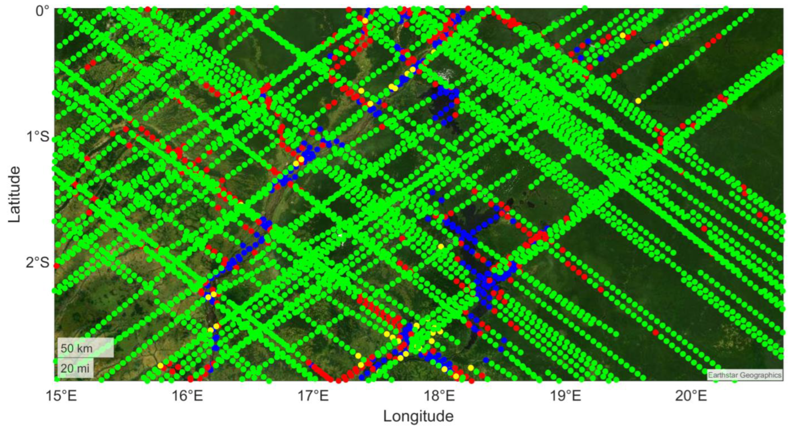
To denote the validation results, four different colors are used. Green points stand for True Negative (TN), where both the clustering result from CYGNSS observation and the Copernicus mask is land, while blue points symbolize True Positive (TP), where in both observations is inland waterbodies. Moreover, red points signify False Positive (FP), where the clustering result is water body in contrast with the Copernicus mask where the result is land. Furthermore, yellow points stand for False Negative (FN), where the clustering result is land whereas the Copernicus mask is water body.
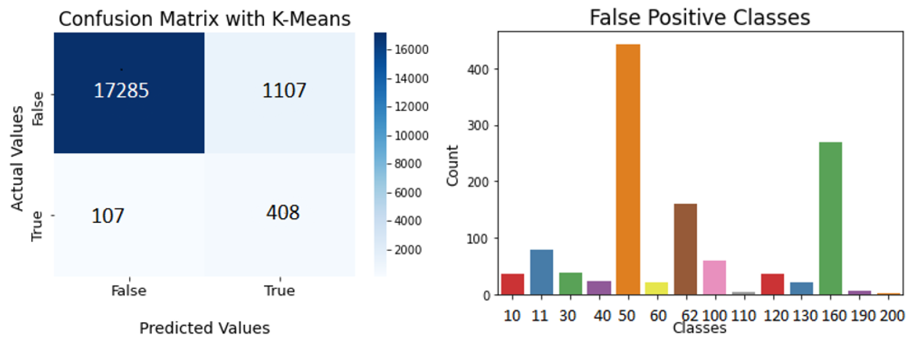
In Figure 8, the evaluation results over the Congo Basin is illustrated using the results of K-means clustering as predicted values. Also, we use confusion matrices, as depicted in Figure 9, to represent the outcomes of validation. The main diagonal of the confusion matrix consists of the number of observations that are correctly clustered. On the other hand, the other entries of the matrix show how many observations of one cluster got mistakenly clustered as the other cluster. Moreover, the score metrics of Accuracy, Precision, and Recall are calculated for the evaluation of the performance of the different clustering algorithms.

Figure 8.
Evaluation results using outcomes of K-Means clustering as predicted values.
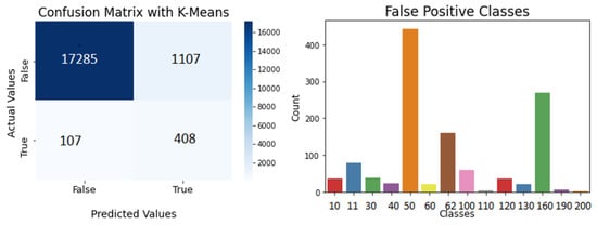
Figure 9.
Confusion matrix using K-Means and false positive classes.
As it can be seen, the Congo River and lakes of the area are detected with high accuracy. However, big number of FP is shown in classes 50 (tree cover, broadleaved, evergreen, closed to open (>15%)) and 160. Class 50 is the most common over the Congo Basin. As described above, class 160 is a mix of tree cover and water, and FP points over this class should be considered as TP. Also, while the Copernicus mask has finer details about the waterbodies it captures, because of the not so high spatial resolution (300 m), smaller tributaries cannot clearly be identified and marked as land. Calculating the score metrics described above, the Accuracy of K-Means algorithm is 93.5%, while of Precision is 26.9% because of the high number of FP. Also, Recall is 79.2%.
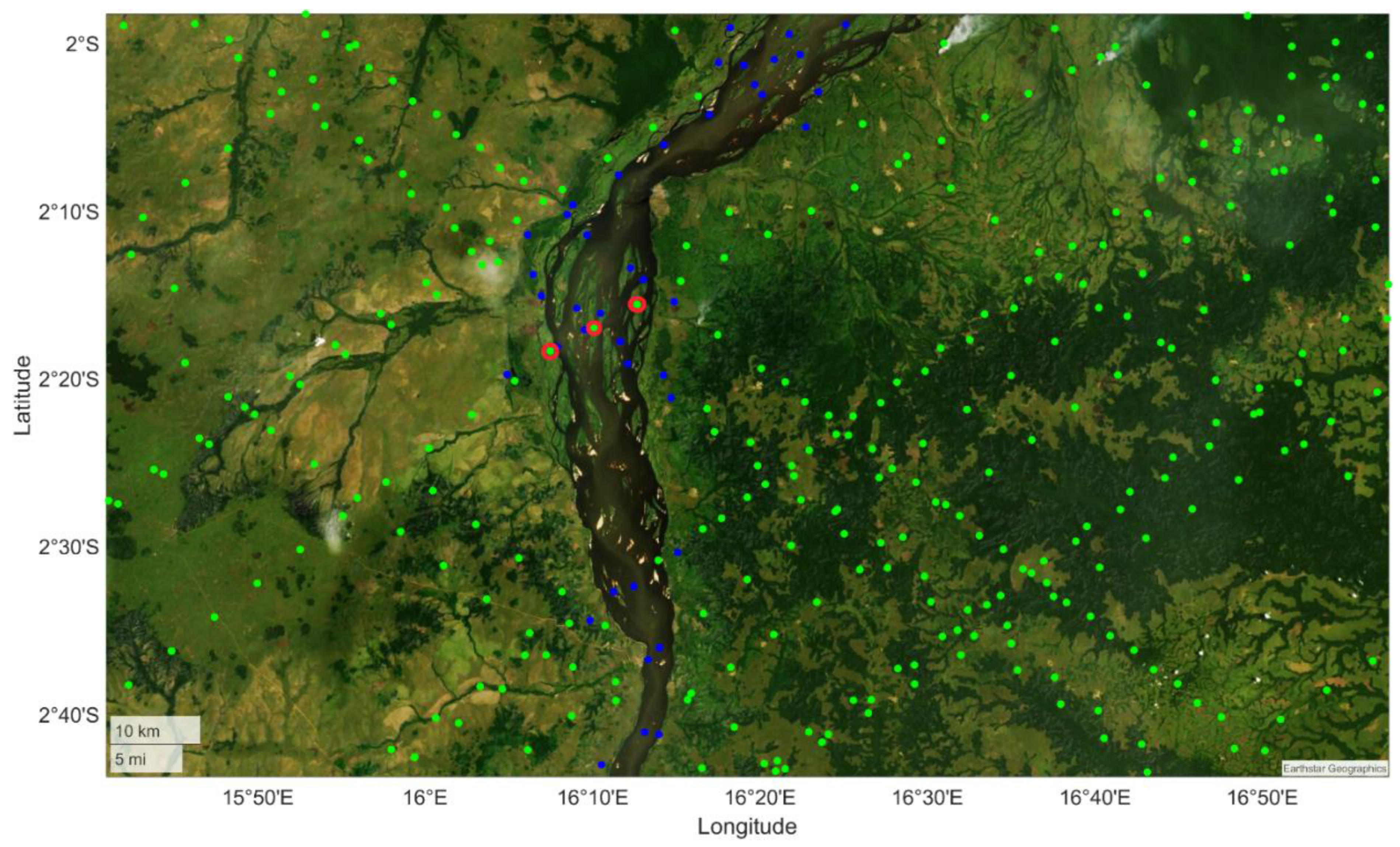
As shown in Figure 10, small tributaries of the Congo River are being detected by the CYGNSS observations using unsupervised ML algorithms, whereas they are not included in the Copernicus land cover classification gridded maps at 300 m spatial resolution produced in the context of the Copernicus Climate Change Service (C3S). It is understood that the spatial resolution of the Copernicus land cover mask is a result of the high number of FP.
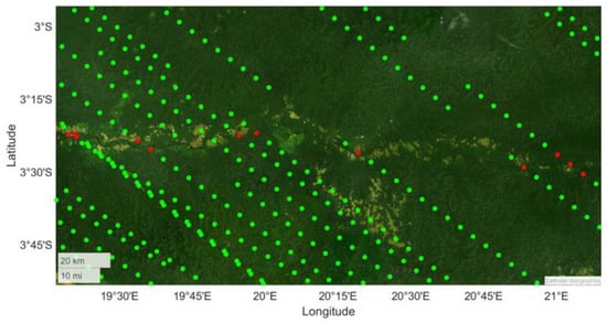
Figure 10.
Small tributaries detected by CYGNSS observations but not by Copernicus land cover mask.
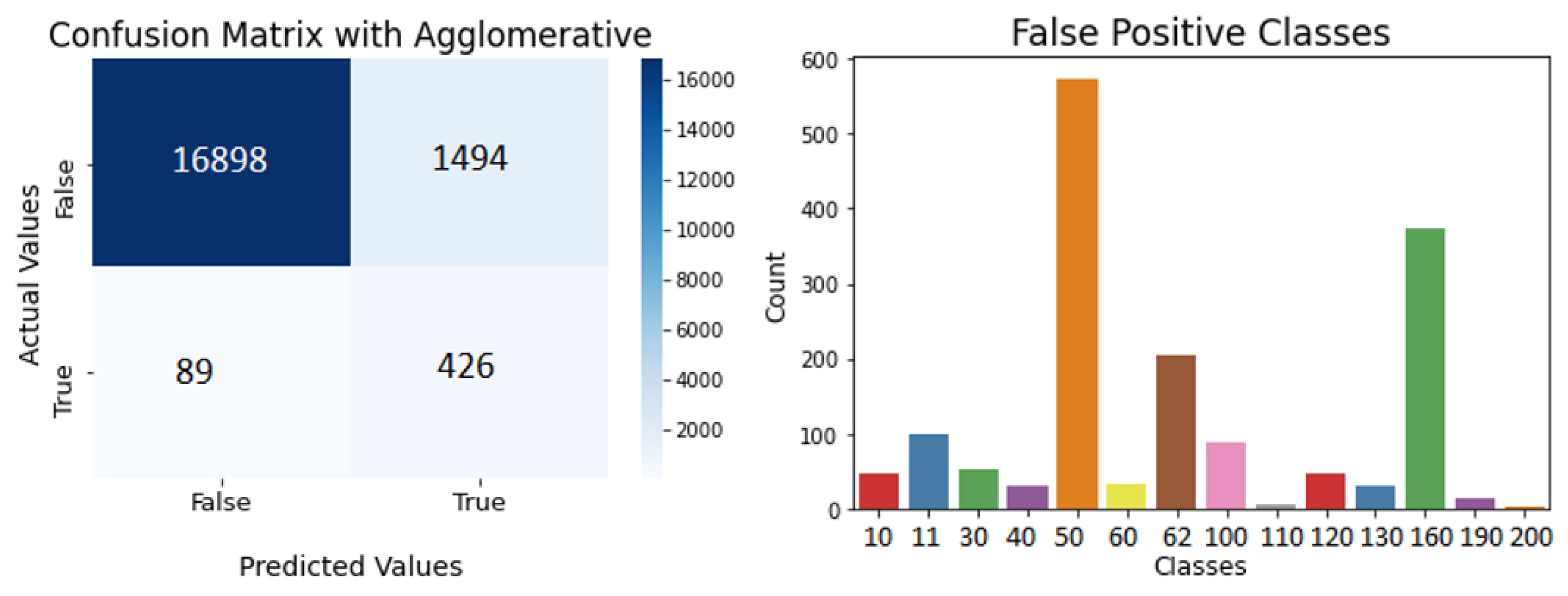
Furthermore, in Figure 11, the evaluation results are predicted, using the results with Agglomerative clustering as predicted values. As it can be seen, Agglomerative clustering detects less TN points than K-Means and higher number of FP. Also, FP outcomes are shown over the classes 50, 160 and 62 (tree cover, broadleaved and deciduous) of the Copernicus map. The Accuracy of the Agglomerative algorithm is 91.6%, while the higher number of FP compared to the K-Means algorithm results in the decrease in Precision (22.2%). Moreover, the Recall is 82.7%, thanks to the decrease in FN compared to the K-Means method.
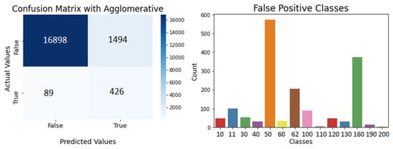
Figure 11.
Confusion matrix using Agglomerative and false positive classes.
The number of inland water bodies detected via the Agglomerative method is slightly higher than K-Means. However, from the confusion matrix, it can be seen that the number of FP is significantly higher than in the K-Means method. Moreover, as in the case of K-Means, the Agglomerative algorithm can detect small tributaries that are not included in the Copernicus land cover mask.
Finally, in Figure 12 the evaluation results are illustrated, using the results with DBSCAN clustering as predicted values. The Accuracy of the DBCAN algorithm is 90.3%, while Recall is 83.1% thanks to the lowest number of FN among the clustering algorithms. The Precision is 19.6%. The number of FP is significantly higher than in the previous methods, while the number of detected inland water bodies is almost the same. There are many observations, over tree cover area, detected as inland water bodies.

Figure 12.
Confusion matrix using DBSCAN and false positive classes.
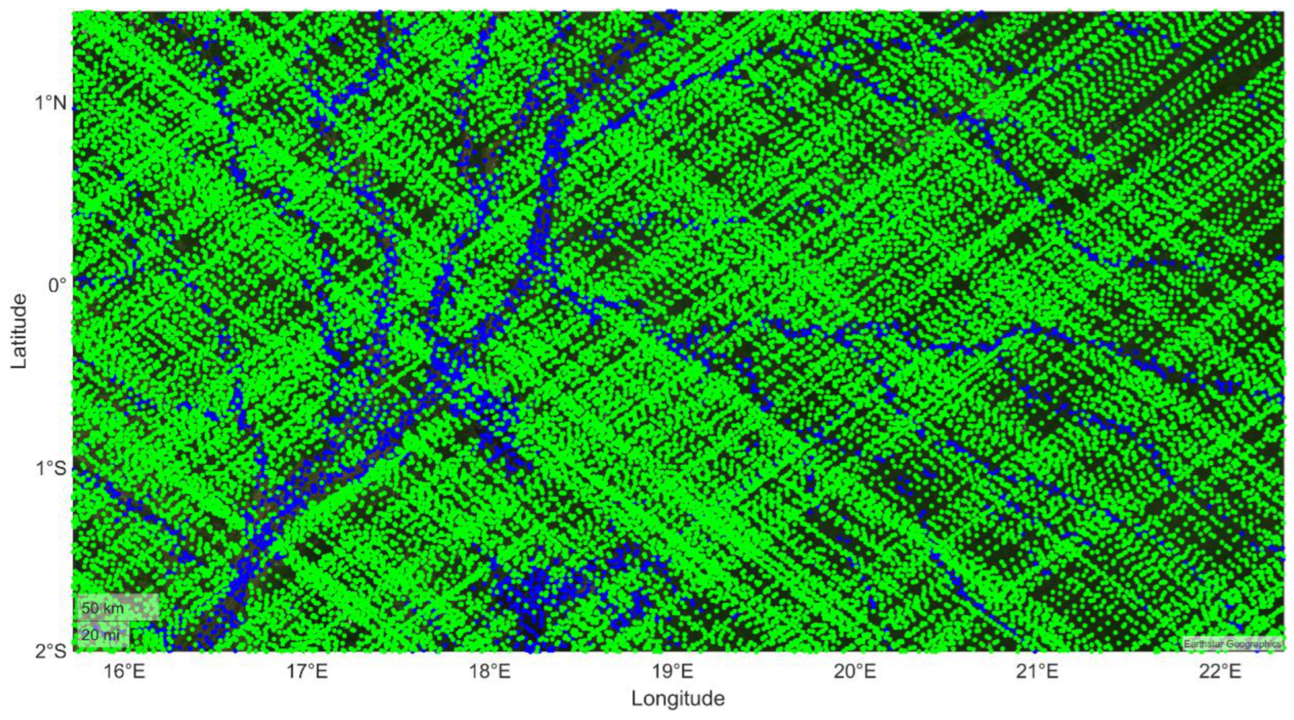
Using ground truth data from the yearly Copernicus land cover map, the K-Means algorithm distinguishes CYGNSS observations between land and inland waterbodies clusters with the highest accuracy. The number of FP detected via K-Means is considerably smaller than in the two other methods, whereas the number of detected inland waterbodies is almost equal. Therefore, in Figure 13, a map over the Congo Basin of the one-month CYGNSS observations, between the 1 and 31 August 2018, using the K-Means algorithm, is depicted. The blue points symbolize observations detected as inland waterbodies, while green points stand for observations over land.
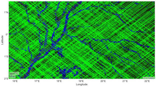
Figure 13.
Map over the Congo basin using 1-month observations (1–31 August 2018).
4.2. Difficulties in Clustering Algorithms
As it is proven, spaceborne GNSS-R is sensitive to different land surface properties, offering the potential to detect and monitor inland water bodies. Unsupervised ML techniques could be used for the mapping of inland water bodies using SNR measurements provided by the CYGNSS constellation. However, the initial analysis of the resulting maps showed three areas wherein improvement is required. The first is related to very high or very low SNR measurements of some tracks that appear to be track-based and not related to surface properties because of the spatial sampling properties of the CYGNSS data (samples taken along one-dimensional swaths) and the multiple CYGNSS and GPS satellites. In [47], the authors explain that these high and low SNR tracks are likely due to the variations in GPS power and will be corrected for the upcoming versions of CYGNSS data. In Figure 14, the red circles denote the false clustering of observations over the Congo River. The current track, as seen in Figure 15, consists of low SNR values, between 0.2 dB and 1.0 dB. These values appear to be track-based and not related to land properties. Observations with red circles should have been clustered as inland water bodies instead of land.

Figure 14.
False clustering because of track-based SNR measurements.
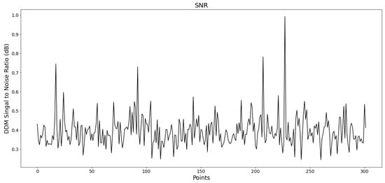
Figure 15.
SNR values not related to surface properties (Track 1056, on 3 August 2018).
The second issue is related to false alarms over desert regions having exceptionally flat surfaces. Implementing the clustering methods over desert regions, such as in Sahara in the North part of African continent and in Rub’ al Khali Desert, shows the weaknesses of the algorithms to detect these areas as land and not as inland water bodies. Thus, the known absence of inland water within these regions enables their removal of CYGNSS observations over these regions to produce maps of inland water bodies. Also, a study reported similar false alarms over deserts in surface water datasets [48]. The last issue is the detection and mapping of large lakes around the globe. This is attributed to the big size of these water bodies. Wind roughening can cause coherence to be no longer the dominant mode of scattering. In Figure 16, the false clustering result over the Tanganyika Lake, the sixth biggest lake in the world, is depicted.
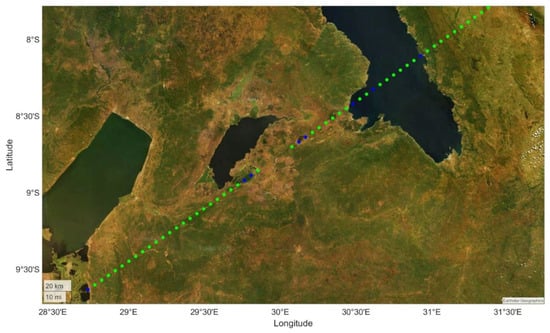
Figure 16.
False clustering over large inland water bodies, such as Tanganyika.
Along the lake, there are only three points clustered as inland water bodies, while eight points are clustered as land instead of waterbodies. The reflected signals close to the shore of the lake create strong coherent features, while at the center of the lake, strong winds result in incoherent scattering signals of approximately 5 dB. Thus, clustering algorithms are unable to detect the inland water bodies. The same results are taken also for the Victoria and Malawi Lake. Hence, it can be understood that the removal of CYGNSS observations over huge lakes around the world is not a solution for the detection and mapping of large lakes, and thus further investigation is required.
5. Summary and Conclusions
Mapping water bodies at a global scale is a challenging task because of the global variety of terrains and water surface. The current study showcases the potential of CYGNSS observations to detect and map inland waterbodies, such as lakes and rivers. A key contribution is the use of unsupervised ML algorithms, such as K-Means, DBSCAN, and Agglomerative, for the detection of inland waterbodies. The application of these algorithms also showed their ability to detect small tributaries, that are missing from the Copernicus land cover classification gridded maps at 300 m spatial resolution produced in the context of the Copernicus Climate Change Service (C3S).
The L-band GNSS signals can penetrate even dense vegetation canopies providing information about water, due to its long radio wavelength. Since GNSS-R is highly sensitive to different land surface properties, both BRCS and SNR can be used to depict the difference between the intensified powers of signals over standing water and over rough surfaces, such as land and oceans. Therefore, we can take advantage of both parameters to identify and map changes in the position and extent of inland waterbodies. Moreover, the short mean revisit time of the CYGNSS observations (7 h) enables the identification of hydrologic phenomena, which evolve at short time windows. The algorithm developed can be employed to make maps on short timescales using weekly, monthly, or seasonal data, in contrast to low temporal resolution water masks of MODIS and Copernicus. However, the density of the CYGNSS observation data could be further improved for mapping purposes. This key issue could be addressed by increasing the number of onboard processing channels, as well as by using reflected signals of other GNSS constellations, such as Galileo, GLONASS, and BeiDou.
Since our approach detects inland waterbodies as long as the reflected signals are predominantly coherent over standing water bodies, we should note that it has trouble identifying deserts as land, because over deserts the strong forward reflection due to the flat surface results in a very strong received signal. Also, due to diffuse scattering over rough water surfaces, big lakes are not detected as inland water bodies on some occasions. The known absence of inland water within big deserts enables their removal of CYGNSS observations over these regions to produce inland water bodies maps. However, additional work is needed in the case of lakes, since roughening wind measurements could also be included to our analysis. Moreover, more information is needed in the case of flat coastal areas since the coherent reflections are detected as inland water bodies.
Furthermore, comparison results on the basis of the Copernicus land cover gridded maps show that unsupervised ML algorithms can be used to monitor and detect inland water bodies with high accuracy at high temporal resolution. The K-Means method has the highest Accuracy (93.5%), compared to the Agglomerative (91.6%) and DBSCAN (90.3%) methods. However, the DBSCAN algorithm has the highest Recall (83.1%), thanks to the lowest number of FN, compared to the K-Means (79.2%) and Agglomerative (82.7%) methods. Moreover, Agglomerative is the most computationally expensive algorithm. Also, in follow-up studies the accuracy of the performances of the algorithms could be improved using quality flags to filter the SNR observations.
The unsupervised ML algorithms presented and implemented in the current study are traditional clustering methods forming the baseline scenario for alternative and novel data-scientific approaches. Therefore, future research should be conducted using additional input data, such as incidence angle and BRCS, creating multidimensional input vectors. Both features could be analyzed to describe either strong diffuse or specular scatterings. Furthermore, follow-up work could be also performed using advanced data scientific methods, such as artificial neural networks, which are expected to provide more accurate results than statistics and traditional clustering methods for the detection and mapping of inland waterbodies. Apart from SNR, BRCS and incidence angle observations, the efficiency of ANN could be examined by adding more features to the input layer, such as the Leading-Edge Slope. Thus, further data preprocessing should be conducted to obtain a more balanced dataset to increase the outcome’s accuracy. Except for the analysis of the different pixel values of DDMs, convolutional neural networks could be used for visual analysis, capturing the essential nature of the identified patterns of DMMs to detect and map inland waterbodies.
Finally, it can be concluded that the current study shows the efficiency of unsupervised ML techniques for the detection and mapping of inland waterbodies. Moreover, it offers valuable experimental outcomes for further investigations and improvement of the methods’ performance. The present findings have major implications in the field of GNSS-R and machine learning, offering valuable insights and analysis for further investigations. With the expectation that CYGNSS will continue to operate and will be followed by future GNSS-R missions, such as HydroGNSS and PRETTY, inland waterbodies maps with higher spatial resolution are expected.
Author Contributions
S.K. and M.A. developed the methodology, conceptualized, and designed the simulations. S.K. performed the simulations, visualized the results, and wrote the original draft. M.A. assisted in the revision process. J.W. supervised and assisted in the revision process. All authors have read and agreed to the published version of the manuscript.
Funding
This research was supported by GFZ—German Research Centre for Geosciences GFZ, 14473 Potsdam, Germany (Grant number: Household).
Acknowledgments
The authors would like to thank the CYGNSS team for providing the CYGNSS data, which are publicly available on the NASA Earth Observing System Data and Information System (EOSDIS) data center. They also thank the Copernicus Climate Change Service for providing the land cover gridded maps, which too are publicly available.
Conflicts of Interest
The authors declare no conflict of interest.
References
- Botzen, W.J.W.; Deschenes, O.; Sanders, M. The Economic Impacts of Natural Disasters: A Review of Models and Empirical Studies. Rev. Environ. Econ. Policy 2019, 13, 167–188. [Google Scholar] [CrossRef]
- Li, Z.; Huang, Q.; Emrich, C.T. Introduction to social sensing and big data computing for disaster management. Int. J. Digit. Earth 2019, 12, 1198–1204. [Google Scholar] [CrossRef]
- Jin, S.; Cardellach, E.; Xie, F. GNSS Remote Sensing: Volume 19 of Remote Sensing and Digital Image Processing; Springer: Dordrecht, The Netherlands, 2014; ISBN 978-94-007-7482-7. [Google Scholar]
- Zavorotny, V.U.; Gleason, S.; Cardellach, E.; Camps, A. Tutorial on Remote Sensing Using GNSS Bistatic Radar of Opportunity. IEEE Geosci. Remote Sens. Mag. 2014, 2, 8–45. [Google Scholar] [CrossRef]
- Postel, S.L. Entering an Era of Water Scarcity: The Challenges Ahead. Ecol. Appl. 2000, 10, 941–948. [Google Scholar] [CrossRef]
- Bastviken, D.; Tranvik, L.J.; Downing, J.A.; Crill, P.M.; Enrich-Prast, A. Freshwater Methane Emissions Offset the Continental Carbon Sink. Science 2011, 331, 50. [Google Scholar] [CrossRef]
- Shao, C.; Chen, J.; Stepien, C.A.; Chu, H.; Ouyang, Z.; Bridgeman, T.B.; Czajkowski, K.P.; Becker, R.H.; John, R. Diurnal to annual changes in latent, sensible heat, and CO2 fluxes over a Laurentian Great Lake: A case study in Western Lake Erie. J. Geophys. Res. Biogeosci. 2015, 120, 1587–1604. [Google Scholar] [CrossRef]
- Blango, M.M.; Cooke, R.A.; Moiwo, J.P. Effect of soil and water management practices on crop productivity in tropical inland valley swamps. Agric. Water Manag. 2019, 222, 82–91. [Google Scholar] [CrossRef]
- Tranvik, L.J.; Downing, J.A.; Cotner, J.B.; Loiselle, S.A.; Striegl, R.G.; Ballatore, T.J.; Dillon, P.; Finlay, K.; Fortino, K.; Knoll, L.B.; et al. Lakes and reservoirs as regulators of carbon cycling and climate. Limnol. Oceanogr. 2009, 54, 2298–2314. [Google Scholar] [CrossRef]
- Kerr, Y.H.; Waldteufel, P.; Wigneron, J.P.; Martinuzzi, J.; Font, J.; Berger, M. Soil moisture retrieval from space: The Soil Moisture and Ocean Salinity (SMOS) mission. IEEE Trans. Geosci. Remote Sens. 2001, 39, 1729–1735. [Google Scholar] [CrossRef]
- Entekhabi, D.; Njoku, E.G.; O’Neill, P.E.; Kellogg, K.H.; Crow, W.T.; Edelstein, W.N.; Entin, J.K.; Goodman, S.D.; Jackson, T.J.; Johnson, J.; et al. The Soil Moisture Active Passive (SMAP) Mission. Proc. IEEE 2010, 98, 704–716. [Google Scholar] [CrossRef]
- Ruf, C.S.; Chew, C.; Lang, T.; Morris, M.G.; Nave, K.; Ridley, A.; Balasubramaniam, R. A New Paradigm in Earth Environmental Monitoring with the CYGNSS Small Satellite Constellation. Sci. Rep. 2018, 8, 8782. [Google Scholar] [CrossRef] [PubMed]
- Chew, C.C.; Shah, R.; Zuffada, C.; Mannucci, A.J. Wetland mapping and measurement of flood inundated area using ground-reflected GNSS signals in a bistatic radar system. Int. Geosci. Remote Sens. Symp. 2016, 2016, 7184–7187. [Google Scholar] [CrossRef]
- Nghiem, S.V.; Zuffada, C.; Shah, R.; Chew, C.; Lowe, S.T.; Mannucci, A.J.; Cardellach, E.; Brakenridge, G.R.; Geller, G.; Rosenqvist, A. Wetland monitoring with Global Navigation Satellite System reflectometry. Earth Space Sci. 2017, 4, 16–39. [Google Scholar] [CrossRef] [PubMed]
- Ruf, C.S.; Gleason, S.; Jelenak, Z.; Katzberg, S.; Ridley, A.; Rose, R.; Scherrer, J.; Zavorotny, V. The CYGNSS nanosatellite constellation hurricane mission. In Proceedings of the 2012 IEEE International Geoscience and Remote Sensing Symposium, Munich, Germany, 22–27 July 2012; pp. 214–216. [Google Scholar] [CrossRef]
- Ruf, C.; Chang, P.; Clarizia, M.P.; Gleason, S.; Jelenak, Z.; Murray, J.; Morris, M.; Musko, S.; Posselt, D.; Provost, D.; et al. CYGNSS Handbook Cyclone Global Navigation Satellite System; National Aeronautics and Space Administration: Ann Arbor, MI, USA, 2016; Volume 148.
- Unwin, M.J.; Pierdicca, N.; Cardellach, E.; Rautiainen, K.; Foti, G.; Blunt, P.; Guerriero, L.; Santi, E.; Tossaint, M. An Introduction to the HydroGNSS GNSS Reflectometry Remote Sensing Mission. IEEE J. Sel. Top. Appl. Earth Obs. Remote Sens. 2021, 14, 6987–6999. [Google Scholar] [CrossRef]
- Wickert, J.; Cardellach, E.; Martin-Neira, M.; Bandeiras, J.; Bertino, L.; Andersen, O.B.; Camps, A.; Catarino, N.; Chapron, B.; Fabra, F.; et al. GEROS-ISS: GNSS Reflectometry, Radio Occultation, and Scatterometry Onboard the International Space Station. IEEE J. Sel. Top. Appl. Earth Obs. Remote Sens. 2016, 9, 4552–4581. [Google Scholar] [CrossRef]
- Cardellach, E.; Wickert, J.; Baggen, R.; Benito, J.; Camps, A.; Catarino, N.; Chapron, B.; Dielacher, A.; Fabra, F.; Flato, G.; et al. GNSS Transpolar Earth Reflectometry exploriNg System (G-TERN): Mission Concept. IEEE Access 2018, 6, 13980–14018. [Google Scholar] [CrossRef]
- Castellví, J.; Camps, A.; Corbera, J.; Alamús, R. 3Cat-3/MOTS Nanosatellite Mission for Optical Multispectral and GNSS-R Earth Observation: Concept and Analysis. Sensors 2018, 18, 140. [Google Scholar] [CrossRef]
- Alonso-Arroyo, A.; Zavorotny, V.U.; Camps, A. Sea Ice Detection Using U.K. TDS-1 GNSS-R Data. IEEE Trans. Geosci. Remote Sens. 2017, 55, 4989–5001. [Google Scholar] [CrossRef]
- Cartwright, J.; Banks, C.J.; Srokosz, M. Sea Ice Detection Using GNSS-R Data from TechDemoSat-1. J. Geophys. Res. Oceans 2019, 124, 5801–5810. [Google Scholar] [CrossRef]
- Strandberg, J.; Hobiger, T.; Haas, R. Coastal Sea Ice Detection Using Ground-Based GNSS-R. IEEE Geosci. Remote Sens. Lett. 2017, 14, 1552–1556. [Google Scholar] [CrossRef]
- Rodriguez-Alvarez, N.; Holt, B.; Jaruwatanadilok, S.; Podest, E.; Cavanaugh, K.C. An Arctic sea ice multi-step classification based on GNSS-R data from the TDS-1 mission. Remote Sens. Environ. 2019, 230, 111202. [Google Scholar] [CrossRef]
- Gerlein-Safdi, C.; Ruf, C.S. A CYGNSS-Based Algorithm for the Detection of Inland Waterbodies. Geophys. Res. Lett. 2019, 46, 12065–12072. [Google Scholar] [CrossRef]
- Carroll, M.L.; DiMiceli, C.M.; Townshend, J.R.G.; Sohlberg, R.A.; Hubbard, A.B.; Wooten, M.R. MOD44W: Global MODIS Water Maps User Guide. Int. J. Digit. Earth 2017, 10, 207–218. [Google Scholar] [CrossRef]
- Li, W.; Cardellach, E.; Fabra, F.; Ribo, S.; Rius, A. Applications of Spaceborne GNSS-R over Inland Waters and Wetlands. In Proceedings of the IGARSS 2019—2019 IEEE International Geoscience and Remote Sensing Symposium, Yokohama, Japan, 28 July–2 August 2019; pp. 5255–5258. [Google Scholar] [CrossRef]
- Rajabi, M.; Nahavandchi, H.; Hoseini, M. Evaluation of CYGNSS Observations for Flood Detection and Mapping during Sistan and Baluchestan Torrential Rain in 2020. Water 2020, 12, 2047. [Google Scholar] [CrossRef]
- Ghasemigoudarzi, P.; Huang, W.; De Silva, O.; Yan, Q.; Power, D. A Machine Learning Method for Inland Water Detection Using CYGNSS Data. IEEE Geosci. Remote Sens. Lett. 2022, 19. [Google Scholar] [CrossRef]
- Al-Khaldi, M.M.; Johnson, J.T.; Gleason, S.; Loria, E.; O’Brien, A.J.; Yi, Y. An Algorithm for Detecting Coherence in Cyclone Global Navigation Satellite System Mission Level-1 Delay-Doppler Maps. IEEE Trans. Geosci. Remote Sens. 2020, 59, 4454–4463. [Google Scholar] [CrossRef]
- Al-Khaldi, M.M.; Johnson, J.T.; Gleason, S.; Chew, C.C.; Gerlein-Safdi, C.; Shah, R.; Zuffada, C. Inland Water Body Mapping Using CYGNSS Coherence Detection. IEEE Trans. Geosci. Remote Sens. 2021, 59, 7385–7394. [Google Scholar] [CrossRef]
- Asgarimehr, M.; Wickert, J.; Reich, S. Evaluating Impact of Rain Attenuation on Space-borne GNSS Reflectometry Wind Speeds. Remote Sens. 2019, 11, 1048. [Google Scholar] [CrossRef]
- Chew, C.C.; Small, E.E. Soil Moisture Sensing Using Spaceborne GNSS Reflections: Comparison of CYGNSS Reflectivity to SMAP Soil Moisture. Geophys. Res. Lett. 2018, 45, 4049–4057. [Google Scholar] [CrossRef]
- Chew, C.; Shah, R.; Zuffada, C.; Hajj, G.; Masters, D.; Mannucci, A.J. Demonstrating soil moisture remote sensing with observations from the UK TechDemoSat-1 satellite mission. Geophys. Res. Lett. 2016, 43, 3317–3324. [Google Scholar] [CrossRef]
- Geremia-Nievinski, F.; e Silva, M.F.; Boniface, K.; Monico, J.F.G. GPS Diffractive Reflectometry: Footprint of a Coherent Radio Reflection Inferred from the Sensitivity Kernel of Multipath SNR. IEEE J. Sel. Top. Appl. Earth Obs. Remote Sens. 2016, 9, 4884–4891. [Google Scholar] [CrossRef]
- Camps, A. Spatial Resolution in GNSS-R Under Coherent Scattering. IEEE Geosci. Remote Sens. Lett. 2019, 17, 32–36. [Google Scholar] [CrossRef]
- Loria, E.; O’Brien, A.; Zavorotny, V.; Downs, B.; Zuffada, C. Analysis of scattering characteristics from inland bodies of water observed by CYGNSS. Remote Sens. Environ. 2020, 245, 111825. [Google Scholar] [CrossRef]
- James, G.; Hastie, T.; Tibshirani, R.; Witten, D. An Introduction to Statistical Learning, 2nd ed.; Springer: Berlin/Heidelberg, Germany, 2021; Volume 102, p. 618. [Google Scholar]
- Pedregosa, F.; Varoquaux, G.; Gramfort, A.; Michel, V.; Thirion, B.; Grisel, O.; Blondel, M.; Prettenhofer, P.; Weiss, R.; Dubourg, V.; et al. Scikit-learn: Machine Learning in Python. J. Mach. Learn. Res. 2011, 127, 2825–2830. [Google Scholar] [CrossRef]
- Müller, A.C.; Guido, S. Introduction to Machine Learning with Python; O’Reilly Media, Inc.: Sebastopol, CA, USA, 2020. [Google Scholar]
- Ester, M.; Kriegel, H.P.; Sander, J.; Xu, X. A Density-Based Algorithm for Discovering Clusters in Large Spatial Databases with Noise. Compr. Chemom. 1996, 2, 635–654. [Google Scholar] [CrossRef]
- Vander, J. Python Data Science Handbook. Volume 53. 2019. Available online: https://jakevdp.github.io/PythonDataScienceHandbook/ (accessed on 1 May 2023).
- Dinh, D.T.; Fujinami, T.; Huynh, V.N. Estimating the optimal number of clusters in categorical data clustering by silhouette coefficient. In International Symposium on Knowledge and Systems Sciences; Springer: Singapore, 2019; pp. 1–17. [Google Scholar] [CrossRef]
- Shutaywi, M.; Kachouie, N.N. Silhouette Analysis for Performance Evaluation in Machine Learning with Applications to Clustering. Entropy 2021, 23, 759. [Google Scholar] [CrossRef]
- Pekel, J.-F.; Cottam, A.; Gorelick, N.; Belward, A.S. High-resolution mapping of global surface water and its long-term changes. Nature 2016, 540, 418–422. [Google Scholar] [CrossRef] [PubMed]
- Lamarche, C.; Defourny, P. Copernicus Climate Change Servise. Product Guide Specification CDR Land Cover (Brokered from CCI Land Cover). 2018. Available online: https://climate.copernicus.eu/ (accessed on 1 May 2023).
- Wang, T.; Ruf, C.S.; Block, B.; McKague, D.S.; Gleason, S. Design and Performance of a GPS Constellation Power Monitor System for Improved CYGNSS L1B Calibration. IEEE J. Sel. Top. Appl. Earth Obs. Remote Sens. 2018, 12, 26–36. [Google Scholar] [CrossRef]
- Schroeder, R.; McDonald, K.C.; Chapman, B.D.; Jensen, K.; Podest, E.; Tessler, Z.D.; Bohn, T.J.; Zimmermann, R. Development and Evaluation of a Multi-Year Fractional Surface Water Data Set Derived from Active/Passive Microwave Remote Sensing Data. Remote Sens. 2015, 7, 16688–16732. [Google Scholar] [CrossRef]
Disclaimer/Publisher’s Note: The statements, opinions and data contained in all publications are solely those of the individual author(s) and contributor(s) and not of MDPI and/or the editor(s). MDPI and/or the editor(s) disclaim responsibility for any injury to people or property resulting from any ideas, methods, instructions or products referred to in the content. |
© 2023 by the authors. Licensee MDPI, Basel, Switzerland. This article is an open access article distributed under the terms and conditions of the Creative Commons Attribution (CC BY) license (https://creativecommons.org/licenses/by/4.0/).

