
DLRW: Dual-Link Weight Random Walk Model for Aquaculture Boundary Extraction by Single-Polarized SAR Imagery

1
School of Geographical Sciences, Liaoning Normal University, Dalian 116029, China
2
National Marine Environmental Monitoring Center, Dalian 116023, China
3
Information Science and Technology College, Dalian Maritime University, Dalian 116026, China
4
School of Computer Science and Artificial Intelligence, Liaoning Normal University, Dalian 116081, China
*
Author to whom correspondence should be addressed.
Remote Sens. 2023, 15(12), 3109; https://doi.org/10.3390/rs15123109
Submission received: 12 May 2023
/
Revised: 9 June 2023
/
Accepted: 12 June 2023
/
Published: 14 June 2023
(This article belongs to the Special Issue Coastal and Littoral Observation Using Remote Sensing)
Abstract
:Coastal aquaculture is undertaken in shallow and usually sheltered waters along the coast, delineated by aquaculture ponds. Illegal usage of coastal aquaculture can lead to conflicts with local communities and environmental problems. Thus, it is necessary to extract the aquaculture boundary to monitor the expansion of coastal aquaculture to the sea. However, it is challenging for most existing algorithms to extract the aquaculture boundary for synthetic aperture radar (SAR) images under a high incident angle (>30 degree) with horizontal transmitted and received (HH) or vertical transmitted and received (VV) polarization. The difficulties come from the following: (1) seawater can be seen on both sides of such boundaries, (2) the contrast of such boundaries is uneven, and (3) the backscattering coefficients in some parts of such boundaries are low. In this paper, a novel dual-link weight random walk (DLRW)-based method is proposed to extract such boundaries. The proposed DLRW is composed of an automatic seed points generation strategy, and the establishment and solving of a random walk model with the dual-link weight. By a coarse-to-fine procedure, DLRW is used to extract the aquaculture boundaries in the whole imagery. Sentinel-1 and GF-3 images in Dalian and Liaodong Bay, China have been used in experiments. Mean offset (MO), root mean square error (RMSE), Overlapped, accuracy within one pixel (WOP), and accuracy within two pixels (WTP) have been used to evaluate the performance with existing methods. Experimental results have demonstrated the proposed DLRW-based method outperforms existing methods in the extraction on aquaculture boundaries. Under the low tide, the DLRW-based method is better than the other two methods with MO, RMSE, Overlapped, WOP, and WTP by at least 5.75 pixels, 10.43 pixels, 2.88%, 11.09%, and 18.04%, respectively. Under the high tide, the DLRW-based method is superior to the other two methods with MO, RMSE, and WTP by at least 3.8 pixels, 10.5 pixels, and 6.3%. In addition, the proposed DLRW-based method has a good ability to extract the shoreline with bedrock, ports, and silt. Therefore, the proposed DLRW-based method can be of great value to coastal aquaculture monitoring, coastal mapping, and other coastal applications.
1. Introduction
The coastal zone is one of the most active and concentrated areas for human life and economic development, but it is fragile to ecology and sensitive to environmental change [1]. In the coastal zone, the coast is composed of aquaculture coast and other coasts such as bedrock, artificial, silty shorelines, etc. As to the former, the boundary between the coastal aquaculture zone and the sea is very important to monitor regarding the expansion of coastal aquaculture. As to the latter, the boundary between land and sea (i.e., shoreline) is very important to monitor regarding the change of coast. The shoreline is an important geographical element identified by the International Geographic Data Commission. Dynamic shoreline monitoring plays an important role in topography mapping [2], ship navigation [3], marine emergency response [4], and other applications, and has important practical significance to promote the sustainable management of the environment, development, and utilization of coastal resources [5]. Many reports can be found on the extraction of shoreline. However, few studies can be found on the extraction of the coastal aquaculture boundary. Hence, it is necessary to seek quick and reliable approaches to extract the boundary of coastal aquaculture.
Most existing research was associated with shoreline extraction. Early shoreline extraction methods mainly relied on field investigation. However, surveying and mapping in some areas was extremely difficult due to the long and tortuous shoreline and constraints of the geographical environment [6]. Remote sensing could provide a solution with its large coverage ability and high spatial resolution, which can realize effective extraction. Among remote sensing data, optical and synthetic aperture radar (SAR) images are the main sources for shoreline monitoring. Optical images have been widely used in shoreline extraction [7,8] due to their abundant spectral information, which can reflect the visual difference directly between sea and land. Nevertheless, it is vulnerable to the influence of cloud cover, solar illumination, and meteorological conditions [9]. On the contrary, SAR images can be used in shoreline extraction regardless of weather and day or night.
In the early stage, shoreline extraction methods in SAR images mainly relied on manual visual interpretation (e.g., direct hand-drawn interpretation [10] or GIS-based vector interpretation [11]). However, this manual approach is time-consuming, labor-intensive, and subjective [12]. Instead, shoreline could be extracted semi-automatically or automatically by computers. It is challenging to extract shoreline because of the nonuniform characteristics of the backscattering signals from the sea surface and the complicated coastal environment [13]. Moreover, the inherent speckle in SAR images is an unavoidable issue [14], which makes the intensity values show considerable variability even in a homogeneous region. Furthermore, imaging factors can also influence shoreline extraction. Baghdadi et al. [15], Ferrentino et al. [16], Wu et al. [17], Kim et al. [18], and Tajima et al. [9] analyzed the effects of wavelength, polarization mode, incident angle, and scene suitability of SAR sensors on shoreline extraction.
Therefore, it is difficult for even experienced interpreters to determine the exact location of the shoreline [19]. According to the existing literature, four kinds of data have been used to extract shoreline: SAR data with auxiliary data, multi-temporal SAR data, multi-polarized (whether dual-polarized or full-polarized) SAR data, and single-polarized SAR data. Using SAR data with auxiliary data (e.g., optical images, light detection, and ranging images, or digital elevation model data) can provide sufficient information for the interpretation of SAR images [20,21,22,23,24]. However, it is a bit difficult at some times to obtain auxiliary data at the same time and region as SAR images. Multi-temporal SAR images could be used to take into account the continuous coastal dynamic change, which is extremely favorable for inter-tidal shoreline extraction and can reduce the effect of speckles to a certain extent [3,4,25]. Nonetheless, extraction with multi-temporal SAR images is based on the assumption of spatial invariance depending on temporal correlation, and errors could occur when the spatial variation is large. Moreover, the acquisition of time–series data is also a problem that should not be ignored. Multi-polarized SAR images could be utilized to combine the statistical characteristics of different channels by the distribution of the coherence matrix [26,27,28,29,30], which can be used to extract shoreline effectively and quickly. In general, multi-polarized SAR images have been successfully applied to shoreline extraction. However, most of the existing methods have limitations in complex sea state conditions [31].
Apart from the above three kinds of data, primarily relying on rich data information, single-polarized SAR images are the easiest and most widely used to extract shoreline. Generally, the shoreline extraction methods of single-polarized SAR images can be divided into several categories, e.g., the edge extraction-based methods [14,32], the threshold-based methods [33,34], the region merge-based methods [35,36], the partial differential equation-based methods [13,37], the deep learning-based methods [2,38], the Markov random field-based methods [39,40], and superpixels-based methods [31,41]. These existing methods have achieved good results under specific conditions and study areas. However, complicated coastal environments, imaging factors, and speckling are still the key to restricting shoreline extraction.
Specifically, the aquaculture coast is one specific coast where most coastal countries develop their aquaculture industry. Coastal aquaculture is undertaken in shallow and usually sheltered waters along the coast. Coastal aquaculture is formed by plenty of adjacent ponds on silt tidal flats. These ponds are constructed with narrow channels with seawater inside. They have similar backscattering coefficients with the sea. In addition, some of them are spatially adjacent to the sea. Coastal aquaculture can provide plenty of seafood. However, illegal usage of coastal aquaculture can lead to conflicts with local communities and environmental problems. The former for common sea space in coastal areas has been intensified not only among the fish farmers but also with other sectors such as shipping, tourism, conservation, and recreation. The latter includes water pollution and the spread of diseases that can threaten native sea life population. Thus, it is necessary to extract the aquaculture boundary to monitor the expansion of coastal aquaculture to the sea. In moderate resolution single-polarized images, especially under a high incident angle condition (>30 degree) and horizontal transmitted and received (HH) or vertical transmitted and received (VV) polarization, the boundary in such aquaculture coast is difficult to extract. Seawater could be seen on both sides of such boundaries. The contrast of such boundaries is uneven, and the backscattering coefficients in some parts of such boundaries are low. Thus, existing methods cannot extract such boundaries well. Up to now, some works on optical images could be seen in Refs [42,43]. However, no report has been found in SAR images. Thus, it is necessary to make a study on such boundary extraction in single-polarized SAR images.
Recently, graph-based methods have been successfully used in shoreline extraction of SAR images, including graph cut [44,45], discriminant cut [46], and normalized cuts [47], which have the advantage of capturing contextual information [48]. The drawback of these algorithms is that they require considerable computational costs and are not efficient in low-contrast regions [47]. As another important graph-based method, random walk (RW) [49] might be a good alternative. By transforming the energy optimization problem into the combinatorial Dirichlet problem, RW can achieve rapid calculation without iteration and has been proven to be advantageous over noise and weak edge response [49]. Moreover, RW can produce an arbitrary extraction result with enough interaction [49] which could meet the requirement of complex coastal scenarios. Researchers have made some important breakthroughs in RW models, including multi-label RW [50], RW with restart [51], lazy RW [52], sub-Markov RW [53], etc. Other related advances mainly involve prior label settings [54,55,56] and weight function improvements [57,58]. Comprehensive reviews of RW have been given systematically in some literature [59,60]. Nevertheless, these RW models are based on the assumption of additive noise and are not robust to speckles in SAR images. The other problem is the local consistency of these RW models, which makes them ineffective for the distorted signals caused by the aquaculture ponds [61]. The backscattering coefficients of aquaculture ponds and sea are nearly identical, separated only by narrow channels which sometimes even fracture in images. Therefore, existing RW-based methods cannot be used directly in aquaculture boundary extraction.
The motivation of this paper is to propose a novel dual-link weight RW (DLRW) method to extract aquaculture boundary. First, an automatic seed points generation strategy is proposed to provide seeds for land and sea. Second, a dual-link weight is proposed that focuses on the similarity of certain special land seeds with the current node and the similarity of the neighborhood to the current node. Third, an RW model on such weight is established. Fourth, a solution to this random walk model is given. Finally, a coarse-to-fine strategy is used to extract aquaculture boundary based on DLRW. Sentinel-1 and GF-3 images in Dalian and Liaodong Bay have been used in experiments. To the best of our knowledge, this is the first study to extract aquaculture boundary from single-polarized SAR images. Meanwhile, no relevant literature has been reported that uses RW to solve aquaculture boundary extraction in SAR images.
The rest of this paper is organized as follows. We first introduce the study area, data description, and pre-processing in Section 2. Then, the proposed DLRW method for aquaculture boundary extraction from single-polarized SAR images is discussed in detail in Section 3. In Section 4, the experimental results are described and analyzed. Our discussion is given in Section 5. Finally, conclusions can be drawn in Section 6.
2. Materials
In this section, we provide the study areas and make a description of the data used in experiments. Then, pre-processing has also been illustrated.
2.1. Study Area
To evaluate the effectiveness and applicability of the proposed method, we selected two study areas. They are located in Liaoning Coastal Economic Belt, with 2290 km of continental shoreline, accounting for about 13% of China. Both are important aquaculture areas in China, with the output of aquaculture accounting for about 14% and 10%. Thus, they are suitable areas to study aquaculture boundary extraction.
The first study area is located in the north of Liaodong Bay, and the administrative area includes Yingkou, Jinzhou, Panjin, and Huludao cities in Liaoning Province, as shown in the upper right image of Figure 1. The coastal zone in this study area is mainly composed of aquaculture, silty, sandy, and bedrock coasts. It is a dense concentration area of aquaculture ponds and ports. The ports include Yingkou and Jinzhou Ports. A large aquaculture area can be seen due to its rich silt coast resources, mainly distributed in Linghai City in the north, Suizhong City in the west, and Bayuquan City in the east.
The second study area is Dalian, a city located at the southern end of Liaodong Peninsula, China, which has a long shoreline surrounded by the Yellow Sea and the Bohai Sea on three sides, as shown in the bottom right image of Figure 1. The shoreline in this study area is dominated by the bedrock shoreline, and the man-made shoreline, with aquaculture boundary. The bedrock shoreline is distributed with capes and bays, making it tortuous and even highly curved. The man-made shoreline is usually composed of complex and dense structures, such as Dalian Port and Dalian Jinzhou International Airport under construction. The aquaculture is mainly distributed on the northern coast of Dalian, where the aquaculture industry has become one of the regional pillar industries because of the abundant marine resources. Specifically, the aquaculture area of Dalian is 467.3 thousand hectares and the output of aquaculture is 1.725 million tons, which accounts for about 8.6% of China, and the scale of aquaculture is at the top of all cities in China.
2.2. Data
Up to now, many spaceborne SAR data can be applied to earth observation, such as Seasat, SIR-B, ERS-1/2, ENVISAT-1, RADARSAT-1/2, and so on. Among them, Sentinel-1 is favored by researchers due to its advantages of high reliability, short revisit time, rapid product delivery, and free data dissemination (the Sentinel-1 images can be accessed at https://scihub.copernicus.eu/ (accessed on 20 November 2022)). The Sentinel-1 is a C-band imaging radar that includes four unique imaging modes with varying resolutions (down to 5 m) and coverage (up to 400 km). Typically, the interferometric wide swath (IW) mode is one of the most widely used among the four operational modes in Sentinel-1 because of its relatively high image quality, i.e., high incidence angle, fine resolution, wide swath width, and optional polarization mode, as listed in Table 1. In addition, for practical use, IW mode has the potential to produce SAR Level 0, Level 1, and Level 2 products. Normally, the Level 1 data are the universally applicable products for the majority of users, and they can be converted to single look complex and ground range detected (GRD). Different from the former, GRD consists of focused SAR data, multi-looked, and projected to ground range using an Earth ellipsoid model which has approximately square spatial resolution pixels and square pixel spacing with speckle reduction. Hence, Sentinel-1 IW GRD data are used as experimental data in this paper.
For the above two study areas, we have chosen the images listed in Table 2. The first image (10,824 × 17,736 pixels) covers Liaodong Bay with VV polarization, which was acquired in September 2022, while the second image (13,212 × 18,236 pixels) covers Dalian with the same VV polarization, which was also acquired in September 2022. It is well known that the position of the shoreline is affected by the level of the tide [62]. In this regard, the two images were chosen in different tidal states. According to the tide level information released by the National Marine Information Center of China (the tide level information can be acquired from http://global-tide.nmdis.org.cn/ (accessed on 12 February 2023)), the first image was taken under high tide conditions and the second image was taken under low tide conditions. These images under different tide conditions can better test the algorithm’s performance. As for the acquisition of ground truth data used for validation, manual interpretation was carried out on ArcGIS software (ArcGIS Desktop 10.8 Advanced-S). Meanwhile, high-resolution Google Maps that coincided with the study images were used for reference and location [63].
2.3. Pre-Processing
The pre-processing of Sentinel-1 images used in this paper was performed using the Sentinel Application Platform (SNAP), which is a common architecture published by European Space Agency (SNAP can be freely downloaded at http://www.esa.int/ESA (accessed on 12 February 2023)). In this paper, we used the Graph Builder module of SNAP to achieve pre-processing. The procedure mainly includes calibration and terrain correction. Before calibration, precise orbit ephemeris data can be automatically downloaded to better remove the systematic error according to applying the orbit file to the original image. Then, calibration is used to convert digital number values into meaningful backscattering coefficients. Finally, to eliminate the range distortion caused by terrain change and sensor tilt, terrain correction is necessary. It is worth noting that the pixel spacing of the images is resampled to 10 m after the terrain correction [64].
3. Methods
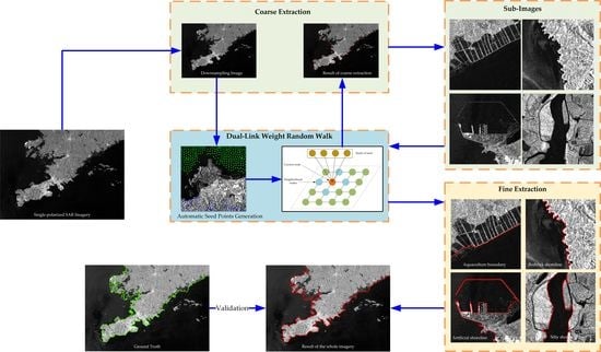
In this section, we present a novel DLRW method to extract aquaculture boundary for single-polarized SAR images, as shown in Figure 2. The proposed method is mainly composed of four steps. The first step is to utilize the proposed DLRW algorithm to extract the coarse shoreline on the downsampling of the original SAR image. The second step is to generate sub-images with shorelines from the original SAR image relying on the coarse shoreline. The third step is to reuse the proposed DLRW algorithm to extract fine shorelines in each sub-image. The final step is to merge the shorelines from all sub-images to generate the shoreline for the whole image. To provide a better understanding of RW theory, we first briefly overview some RW methods. Then, we make a detailed analysis of the proposed DLRW algorithm for SAR images. Finally, the architecture of aquaculture boundary extraction by a coarse-to-fine strategy is provided. Due to the high percentage of shoreline in the whole image, shoreline has been used in Figure 2, where part of it should be aquaculture boundary. In the following sections, for convenience, we take the same description as shoreline, especially for the whole image.
3.1. Overview of RW
Here, we introduce several RW methods. Given an image with , a weighted graph could be generated by nodes, connected by a series of edges with an associated weight matrix . is a set of nodes with each node representing the -th image pixel in . Any edge that belongs to connects two nodes and in a 4- or 8-connect neighborhood. The weight provides similarity between nodes and . Generally, the most widely used weights have been constructed as a function of a difference between two image pixels, which can work well in the additive model, such as optical images. Such weight can be defined as:
where and are two image intensity values in two nodes and . is a user-defined parameter. Then, the degree of a node can be calculated as for the nodes in the neighborhood of (not including itself except for a self-loop case). In addition to such weight, can be composed of a set of labeled nodes and unlabeled nodes . If the labeled nodes can be defined as , then some labels can be denoted as , with as the number of labels. can be regarded as seed points with a label with as the number of seeds. According to the weight, labeled seeds, and the degree, Grady [49] proposed an RW algorithm with Markov transition probability to denote the probability of node under the label as:
where means a node in the neighborhood of node , and could be 4 or 8 representing neighborhood size, with . The final segmentation result for is obtained as:
This RW mainly focuses on the neighbor characteristic of a node. However, it cannot solve some problems such as texture, weak edges, or twigs. Therefore, some other RW algorithms place certain information in connection with labeled nodes or additional items. Here, we could not list all algorithms, and just provide four typical ones. The following two algorithms could provide connections with the labeled nodes by a certain constant. For the -th seed node, Kim et al. [51] proposed a steady-state probability assigned to each node formulated as:
where is a constant between 0 and 1. This algorithm provides a constant connection between each node and the labeled node. Wu et al. [65] proposed a partially absorbing RW model, with its probability to each node as:
where denotes the probability that walks out of the node , and is a constant. The above two RW algorithms have built connections on labeled nodes. The other two RW algorithms involved additional items. The former added auxiliary nodes. Dong et al. [53] proposed a sub-Markov RW algorithm with prior items to formulate its probability of each node as:
where is a constant. denotes the probability density belonging to a label at the node . is the sum of . The latter added a KNN-based weight into an RW model. Yuan et al. [66] proposed a nonlocal random walk algorithm with its probability to each node as:
where denotes to make a connection of an edge by KNN of the node using their feature vectors. is constructed by the intensity difference and spatial difference on KNN to the node . The motivation to use KNN is that when local propagation fails, the KNN can play a leading role in the diffusion.
The above RW algorithms have demonstrated good ability in optical image segmentation. However, these algorithms could not work well in aquaculture boundary extraction in SAR images. There are three reasons. First, the similarity in weight of these algorithms is suitable for the additive model while not useful in the multiplicative model. Second, the connections between the current node and the different labels or additional items can cause erroneous extraction of dams in the aquaculture boundary. The reason is that the former two algorithms built connections on labeled nodes provide an almost equal role for the current node to the labels in land and sea. The latter two algorithms with additional items are based on the additive model. Third, seed points initializing methods are not suitable for aquaculture boundary extraction. To circumvent such drawbacks, it is necessary to study a novel RW algorithm for aquaculture boundary extraction in SAR images.
3.2. Dual-Link Weight Random Walk
In this section, we present an automatic seed points generation strategy and a novel RW method for aquaculture boundary extraction in SAR images. Given an image , we first give descriptions of seed points. Seed points can provide help for the solution of RW. As to the SAR image with the aquaculture boundary, the number of labels is 2, denoted as , with the set of labeled nodes as . If and refer to labels of land and sea, respectively, it is important to obtain two kinds of seed points for . Here, we present an automatic seed points generation strategy for land and sea.
3.2.1. Automatic Seed Points Generation
To generate seed points of land and sea, a direct approach is to make a segmentation between land and sea. Up to now, some research has been reported on SAR image segmentation based on pixels or superpixels. However, the motivation in this section is to obtain definite regions of land and sea, not the accurate segmentation results between land and sea. It means the intersection regions of land and sea should not be considered. Thus, most segmentation methods cannot be used. Here, we present a coarse segmentation method based on superpixels. In contrast to pixel-based methods, superpixel-based methods have prominent advantages. Superpixel-based methods are typical region segmentation methods, grouping pixels into perceptive atomic regions, which can be used to replace the rigid structure of the pixel grid [67]. The simple linear iterative clustering (SLIC) algorithm [67] is one of the most widely used methods due to the advantages of simplicity and efficiency and has been used in the application of SAR images [31]. Therefore, we use SLIC to generate superpixels. To make the segmentation on SAR images, we should study the characteristics of superpixels on land and sea. For the image with a high incident angle (>30 degree) and VV or HH polarization, the mean values of superpixels on the sea are relatively low, and the mean values of superpixels on land demonstrate large-scale dynamic change. If we regard the mean value of each superpixel as a unit, the standard deviation in the adjacent neighbor of the current superpixel multiplied by the mean value of the current superpixel could be used to distinguish land and sea on a coarse scale. We could compute these standard deviations in an image by superpixels. Then, the product of all standard deviations with their corresponding mean values in this image could be arranged in a sequence of ascending order. We choose 10% of the head and 20% of the tail where the head refers to the part of the lowest values, and the tail refers to the part of the highest ones. In the part of the head, we set the maximum connected domain as the sea with each center pixel in each superpixel as a seed point. In the part of the tail, we choose the first 30% of the connected domains farthest from the sea, as land with each center pixel in each superpixel as a seed point. Thus, seed points of land and sea could be denoted as and , where represents the number of seeds on the land, and denotes the number of seeds in the sea. Thus, the generation of seed points for land and sea has been completed.
3.2.2. An RW on Dual-Link Weight
Generally, a weight measures the similarity between node and node . In optical images, can be generated by an exponential function of an intensity distance measure between intensity values in and . However, it is recommended in SAR images to use the ratio between mean intensity in and [68], and could be defined as:
where represents the mean intensity of a pixel patch in node , and can be replaced by the intensity value . is a controlling parameter. In most RW methods, could provide similarity between the current node and its adjacent node. However, such a definition breaks the link of the current node with the labeled node causing the probability of the node being far away from the labeled node low. Therefore, it can result in erroneous segmentation results. Thus, we construct a new weight based on local similarity, and the similarity of the current node with the labeled node, as shown in Figure 3. One link is to build a connection between the neighborhood nodes and the current node. The other link is to make a connection between the specific seeds of nodes and the current node. We defined this weight as:
where is a special seed points set that contains the smallest land seed points in with the same number of points as that of , and is a constant to balance the similarity between labeled nodes to the current node, and the similarity between neighbor nodes to the current node with in this paper. is a constant in most RW methods. However, this parameter has a great effect on the segmentation result of RW. It means that an improper value on can cause incorrect segmentation results. Thus, it is necessary to analyze the influence of on weight. If we define that measures the similarity of nodes and , this similarity on all nodes can be generated into a set from 0 to in an ascending order, which denotes the minimal similarity of two adjacent nodes in an SAR image. On a fixed except 0, a large means a small weight and a small means a large weight in (9). On a fixed , a large means a large weight range for all weights in this image. A large weight range can increase the reaching probability differentiation that may obtain good segmentation by RW. To reduce the influence of a few very large that are sometimes caused by outliers, we construct a histogram of similarity between two adjacent nodes on all nodes by 1000 bins with as the x-axis and choose as the first value of the histogram close to zero from its maximal value. Then, we define a constant in this case as , where is set as in this paper. Then, we could obtain . Thus, the degree of node , can be formulated as:
In this regard, we define the transition probability based on (10) as follows:
Then, the reaching probability of node to node can be denoted by:
where . Thus, the vector notation is formulated as follows:
where is a diagonal matrix whose diagonal element is . is an -dimensional indicator with if and otherwise. is an identity matrix. The transition matrix is a row-normalized matrix with defined at (11).
From (13), a vector formulation of this average steady-state probability can be denoted as follows:
where is a constant used to normalize. Finally, the final segmentation result could be obtained by (3) and (14).
If an optimization explanation is required, Equation (14) could be converted into the following objective function:
Similar to the idea of traditional RW [53], we use (9) and define the combinatorial Laplacian matrix as:
Then, the Dirichlet problem formulation (14) can be rewritten as:
If we need to find a solution for (17), the nodes can be re-arranged into two parts: marked nodes and unmarked nodes . We rewrite the Dirichlet problem of (17) as:
Differentiating (18) with respect to , we obtain:
From (19), we obtain the probabilities of pixels belonging to the seed points. Naturally, the probabilities indicate the similarities of pixels to the seeds. Then, the unlabeled node can be assigned to a label with a larger probability between the probabilities of land and sea.
3.3. Architecture of Aquaculture Boundary Extraction
In this section, we present the process of aquaculture boundary extraction for the whole image by the DLRW method. To reduce the computation burden when the image is oversize, a coarse-to-fine technique has been used.
3.3.1. Coarse Extraction of Shoreline
For the whole SAR image, the percentage of shoreline in an image is relatively low. If a large image is involved in computation on shoreline extraction, the computation burden and computer capability have to be seriously considered. To reduce this burden, this paper takes a similar trick as other shoreline extraction methods [31]. A downsampling technique has been used. If an image is in size, the downsampling image could be obtained by a block of to one pixel. is set to 5 in this paper. Then, the DLRW model is used to extract the aquaculture boundary. Thus, the coarse shoreline map is produced.
3.3.2. Sub-Images Cutting
In this section, this paper provides the technique to automatically obtain sub-images with shorelines in the whole image that are based on a coarse shoreline map. First, each pixel in a coarse shoreline map can be used to locate the position in the whole image by its position and . Then, such position is used as the center to form a block of in the whole image to obtain each sub-image that contains the shoreline. Here, all sub-images are overlapped in the whole image. Therefore, a series of sub-images seems to be cut from the whole image.
3.3.3. Fine Extraction of Shoreline for the Whole Image
This section used the proposed DLRW method to extract the shoreline in each sub-image. If the overlapped shorelines are met, their locations are computed by their mean values. Then, all shorelines in sub-images can be connected in sequence to produce the shoreline in the whole image. Thus, the shoreline in the whole image can be extracted.
3.4. Accuracy Assessment
To better quantify the accuracy of shoreline extraction, five representative assessment indexes, including mean offset (MO) [63], root mean square error (RMSE) [42], overlapped [36], accuracy within one pixel (WOP) [36], and accuracy within two pixels (WTP) [36] are deliberately chosen in this paper. If the extracted shoreline is with as the number of extracted pixels on the shoreline, and the manually marked shoreline is with as the number of manually marked pixels on the shoreline, then the first two indexes can be calculated as:
and
Apparently, the smaller the MO and RMSE, the better the algorithm extraction performance. Then, for the last three indexes, there is a general formula for calculating as:
where is a judgment function (i.e., equals 1 when its independent variable is true and equals 0 otherwise), represents a specific index, and is a natural number. Note that when is 0, 1, and 2, then corresponds to Overlapped, WOP, and WTP, in order. The difference is that the greater the latter three indexes, the higher the extraction accuracy.
4. Results
In this section, we provided experiments to evaluate the DLRW for aquaculture boundary extraction. We first compared and analyzed the results of the DLRW with the existing shoreline extraction algorithms. Then, the extraction results of the whole images by the DLRW were presented and compared with the ground truth to verify the extraction capability.
4.1. Performance Comparison
In this section, the performance comparison of the proposed DLRW algorithm with the existing shoreline extracting algorithms was provided. Here, two shoreline extraction algorithms have been chosen. The first one is the multi-region level set partitioning (MLSP) proposed by Ayed [69]. The other is a superpixel-based shoreline extraction algorithm (SPEC) proposed by Shi [31]. All algorithms have been implemented by MATLAB 2016a on a machine with Intel(R) Core (TM) i7-9850H CPU 2.60 GHz, 32 GB RAM.
First, we made a description of the parameter’s settings for each algorithm. For our DLRW, two parameters are required to be determined, i.e., the estimated superpixel size and . We set the size of the estimated superpixel at 20 because we should make a balance between the coarse segmentation of land and sea and the running speed. As has a significant influence on the extraction results, we fix it to in all experiments and discussed its sensitivity in the following section. In the MLSP, the regularization parameter was set to 0.2. As for the SPEC algorithm, the total direction of edge strength, the window size, the estimated superpixel size, and the expected numbers of Gaussian functions were set to 16, 11, 10, and 20, respectively, which were almost consistent with the recommended parameters. It is worth noting that both the DLRW and SPEC have the same parameter (i.e., estimated superpixel size), and they are set differently. The reason is that SPEC relies on the estimated superpixel size to make superpixels adhere to the shoreline. The smaller this parameter is, the more adhered the superpixels are. Such a setting could cause a computation burden. To give a relatively fair comparison, the estimated superpixel size of SPEC needs to be set small to obtain better performance, which is not required for the DLRW method.
To visually demonstrate the aquaculture boundary extraction performance among three methods, we selected a region ( pixels) from the first study area as shown in Figure 4b, which was located in Jinzhou city, north of Liaodong Bay (marked with a red rectangle in Figure 4a). For the convenience of comparison and verification, Figure 4c shows the shoreline by manual interpretation (marked with green lines). Figure 4d–f are the extraction results of DLRW, SPEC, and MLSP, respectively (marked by the red lines). In general, all the algorithms can obtain acceptable results for aquaculture boundary extraction.
To make a comparison of the three algorithms more clearly and directly, we have selected three typical small regions (marked as A–C with red rectangles in Figure 4b), with zoomed images as shown in Figure 4g–i. Region A showed a part of the aquaculture area adjacent to the sea. It can be seen that all the algorithms can extract aquaculture boundary. The reason is that tidal flat is not obvious under high tide conditions and the dams in the aquaculture area are clear enough. However, for long and thin ditches with aquaculture ponds on two sides, the SPEC method cannot obtain satisfactory results because superpixels do not adhere to the dams, causing subsequent incorrect extraction. Regions B showed part of two adjacent aquaculture areas. DLRW and MLSP demonstrate good results, while SPEC produces some errors for the same reason as in Region A. Region C is composed of a dam and part of an aquaculture area. DLRW can extract aquaculture boundary well. SPEC can produce a jagged aquaculture boundary because of poor fit. MLSP can produce a large aquaculture boundary deviation due to the similarity of sea and aquaculture areas. From Figure 4d–f, DLRW cannot extract one part of the aquaculture boundary. SPEC cannot extract three parts, and MLSP cannot extract two parts. Thus, DLRW demonstrates the best extraction ability for aquaculture boundary.
To quantitatively evaluate the aquaculture boundary extraction performance of three algorithms, MO, RMSE, Overlapped, WOP, and WTP have been used in Table 3. The proposed DLRW algorithm outperforms the other two algorithms in MO and RMSE by around 3.8 pixels and 10.5 pixels, respectively. From Table 3, MLSP is better than SPEC. The main reason is that SPEC depends on the quality of the superpixels, and the superpixels do not adhere well in some complex regions. It is worth noting that Overlapped and WOP of DLRW are less than those of MLSP. It could be seen from the experimental results that MLSP can obtain more fitting results in some regions with high contrast. Nevertheless, within the tolerance of two-pixel intervals, our DLRW is 6.3% greater than MLSP on WTP, demonstrating better results.
To make a further visual comparison, we have chosen a region ( pixels) from the second study area in Wafangdian City, Dalian, Liaoning Province, China, from the red rectangle area in Figure 5a, as shown in Figure 5b, that was utilized to verify the performance comparison among three algorithms for aquaculture boundary extraction under low tide conditions. It could be seen from Figure 5g that all algorithms can achieve extraction results for aquaculture boundary with obvious dams. However, when the boundaries between the sea surface and the aquaculture surface were inconspicuous due to the weak backscattering of the aquaculture dams, both MLSP and SPEC could produce incorrect results, and our proposed DLRW method was able to obtain good results that were more consistent with the ground truth as shown in Figure 5h. The reason was that the contrast was low so that the MLSP could cross the boundary and continue to evolve, while the SPEC already generated errors at the superpixels generation stage. Our DLRW method increased the probability that the aquaculture area belongs to the land by dual-link weight between the land seeds with the unlabeled points, which could effectively extract the aquaculture boundary. In Figure 5i, both DLRW and SPEC can obtain good results under low tide conditions, because DLRW used log-ratio similarity metric and SPEC used Gabor features, while MSLP showed incorrect extraction results due to its similarity in its function.
From Table 4, the DLRW method was superior to other methods with MO, RMSE, Overlapped, WOP, and WTP by at least 5.75 pixels, 10.43 pixels, 2.88%, 11.09%, and 18.04%, respectively. The reason is that MLSP and SPEC produced some uncorrected results in the aquaculture boundary extraction, and MLSP was also inapplicable in the low tide aquaculture boundary. Both of them can be influenced by the presence of intertidal areas. However, the proposed DLRW method could provide better results.
4.2. Performance Evaluation of Whole Image
In this section, we demonstrated extracted shorelines by the DLRW method from the whole images in Dalian and Liaodong Bay, China. In Figure 6, the proposed method is in agreement with the ground truth on the whole which could be seen from the results in bedrocks at the bottom left side and aquaculture ponds at the right side. However, the coastal environment in Dalian is very complex because it is composed of a large number of aquaculture ponds on the upper left and upper right sides, an airport under construction in a rectangular shape, mud flat, narrow channels, etc. It could be seen that some narrow channels in the upper left side cannot be effectively extracted. In addition, the airport in the left center is only extracted with its outer contour which is different from the ground truth.
In Figure 7, the coastal environment is also complicated with ports, several aquaculture ponds, and an estuary, etc. In general, the proposed DLRW method shows a good result on shoreline extraction compared with the ground truth. It could be seen on the upper and right sides of the shoreline that the proposed DLRW method can work well in the extraction of aquaculture ponds and ports. However, some narrow channels in a river and estuary and several dams cannot be well extracted.
From the above analysis, the proposed DLRW has a satisfactory ability to extract the aquaculture boundary under a complex coastal environment.
5. Discussion
5.1. Discussion of DLRW Applied to GF-3 Images
The satellite of GF-3 was launched in 2016. GF-3 is a C band multi-polarization SAR satellite with high resolution, large imaging width, high radiation accuracy, multiple imaging modes, and long hours of operation [70]. GF-3 has 12 kinds of imaging modes, such as spotlight, strip, scan, wave, and global observation [71]. In this paper, two typical modes, namely fine strip II and standard strip, have been selected, and the detailed information can be seen in Table 5. GF-3 data, released by National Satellite Ocean Application Service, contain Level 1 and Level 2 products. The Level 1 data are oversampled complex data products, which should go through the mode operation and radiometric correction to convert digital number values into backward scattering coefficients [72]. The images used in this paper are Level 2 data, for which only geometric correction is required as the pre-processing step. Thus, we used the built-in remote position control file to conduct the system-level geometric correction [73].
To test the availability of the DLRW algorithm to other SAR images, two-scene GF-3 SAR images were selected in this section. The first scene GF-3 image is located in Dalian, China, which is the HH polarization image in fine strip II mode acquired in 2019, and the resolution is m. The second GF-3 image is located in Liaodong Bay, China, which is the VV polarization image in standard strip mode acquired in 2021, and the resolution is m. The extraction results by DLRW can be seen in Figure 8. To provide good visual extract results, two aquaculture areas, and one aquaculture area have been chosen from the first scene, and the second scene, respectively. As can be seen from Figure 8a, DLRW has good adherence to the tortuous aquaculture boundary in GF-3 images. In low sea–land contrast conditions as shown in Figure 8b, DLRW can extract aquaculture boundary well. In Figure 8c, we can see that DLRW can correctly extract aquaculture boundary despite the speckle on the sea surface. Therefore, DLRW can also be used to extract aquaculture boundary on GF-3 SAR images.
5.2. Discussion of DLRW Applied to Other Types of Shoreline
In this section, this paper demonstrates the shoreline extraction ability with the coast of bedrock, silty, artificial shoreline such as an airport and ports. Shoreline with bedrock could be well extracted as shown in Figure 9a,b. As to the silty shoreline in Figure 9c, most have been efficiently extracted except the section adjacent to an island in the sea. In Figure 9d, the airport’s outer contour can be extracted with some narrow channels inside missed. In Figure 9e,f, most ports can be well extracted. Breakwaters can be seen in both images. In Figure 9f, a port built by reclamation can be seen in the middle part, and some artificial ports with breakwaters can be seen in the right middle part. However, two parallel breakwaters can only be extracted partly in the right middle part. On the whole, DLRW can work well in extraction for various kinds of shorelines.
5.3. Discussion of Three Algorithms on Bedrock Shoreline Extraction
To make a comparison of bedrock shoreline extraction for three algorithms, we choose two regions with bedrock shoreline from the image in Dalian, China, as shown in Figure 10a,b. From these two images, three algorithms can extract bedrock shoreline well. However, MLSP can demonstrate some fluctuations in the boundary where the contrast between sea and land is not obvious. The reason is that MLSP can evolve into a small number of land areas when the backscattering of land is a bit low, as shown in the middle and upper part of Figure 10a, and the middle part of Figure 10b. MLSP can evolve into a small number of sea areas when the backscattering of sea is a bit high, as shown in the upper part of Figure 10a. SPEC shows the result slightly off shore. The reason is that superpixels cannot produce good adherence. DLRW can demonstrate better extraction for bedrock shoreline.
5.4. Discussion of DLRW Applied to Cross-Polarization Images
To validate DLRW on cross-polarization SAR images, we choose three sites from an HV image obtained in September 2022 in Dalian, China. The result of extracting the aquaculture boundary can be seen in Figure 11a. DLRW can produce a good result. As to the artificial shoreline as shown in Figure 11b, most shoreline can be extracted well by DLRW. However, three dams can only be partly extracted in the lower left and lower middle part of this image. As to the bedrock shoreline in Figure 11c, DLRW can generate good results.
5.5. Parametric Sensitivity Analysis
In this section, we analyze the parameter sensitivity. The most important parameter in the proposed DLRW method is λ. On a fixed similarity, a large λ can produce a small weight causing low discrimination in reaching probability on the labels of land and sea. On the contrary, a small λ can provide a large weight that provides a large discrepancy in reaching probability on the labels of land and sea.
To find the interval of λ for which the DLRW method has a good performance, a coarse-to-fine trick on an interval has been exploited. In Figure 12, performance is composed of five indexes: MO, RMSE, Overlapped, WOP, and WTP. In Figure 12a,c, the performance refers to the former two indexes based on pixels. In Figure 12b,d, the performance refers to the latter three indexes based on percentage. At a coarse scale, the interval in [0, 1] is used. In Figure 12a, the less MO and RMSE, the better the performance. It can be seen that the interval around should be better. In Figure 12b, the greater Overlapped, WOP, and WTP, the better the performance. The good interval seems to be between and . It is worth noting when , which means that the link between the label points and the current points is disconnected, our method is downgraded to the original RW with modified automated seed points and weights. We could find that the performance is best around in the coarse interval. Thus, it is suggested that a good interval on a small scale for λ should be chosen in . Then, we evaluate λ with this interval in a fine scale. In Figure 12c, we can see that when λ is between and , MO can reach nearly two pixels, while RMSE is within five pixels. In Figure 12d, we can find that when λ lies between and , Overlapped, WOP, and WTP can reach the local peak. Thus, we find that is a compromised value used in this paper.
5.6. Limitation Analysis
In this paper, the proposed DLRW method has shown a good ability to extract aquaculture boundary. In addition, it can be used to extract shoreline of bedrock, man-made shoreline such as ports, and silty shoreline. It is still worth noting that some limitations should be considered. First, narrow channels in outlets or rivers to the sea cannot be well extracted. Second, offshore floating rafts can cause a negative influence on shoreline extraction. Third, some ditches in offshore objects such as an airport in the sea cannot be well extracted. Fourth, the vessels and strong waves may influence the results of shoreline extraction. Therefore, it is important to make a thorough study to solve the limitations mentioned above in the future.
5.7. Future Improvement
Although we have proposed a DLRW method to extract aquaculture boundary in single-polarized SAR images, some limitations should be considered in future work. It is suggested to involve some prior information in the RW model to increase extraction ability on narrow channels, offshore floating rafts, or certain targets such as an airport in the sea. In addition, some preprocessing tricks may be a good way to reduce the influence of vessels and strong waves.
6. Conclusions
In a high incident angle (>30 degree) and VV or HH polarization, aquaculture boundary in moderate single-polarized SAR image generally demonstrates discontinuity and low contrast. Thus, it is a difficult problem to extract such aquaculture boundaries, and no study has been found on this issue so far. This paper proposes a DLRW method to extract aquaculture boundary in single-polarized SAR images. First of all, an automatic seed points generation strategy is proposed that provides definite seeds for land and sea by superpixels. Then, two kinds of weight have been proposed. One is based on the similarity of local nodes to the current node. The other is from the similarity of the smallest land seeds and the current node. Moreover, the combinatorial Laplacian matrix is used to construct the RW model. Furthermore, the solution to this Dirichlet problem is given. Depending on Sentinel-1 images, Dalian and Liaodong Bay have been chosen. Under high tide, experimental results have shown that the proposed DLRW method is superior to SPEC and MLSP methods by at least 3.8 pixels in MO, and 10.5 pixels in RMSE. In WTP, the DLRW method is better than SPEC and MLSP methods by at least 6.3%. Under low tide, the DLRW method is superior to the other two methods with MO, RMSE, Overlapped, WOP, and WTP by at least 5.75 pixels, 10.43 pixels, 2.88%, 11.09%, and 18.04%, respectively. In addition, the proposed method shows good extraction ability in GF-3 images. Moreover, the DLRW method also demonstrates good extraction results on shorelines of bedrock, man-made, and silt. As to the parameters in this method, all parameters have been set automatically except λ. It is suggested to be . However, some limitations should be considered such as narrow channels at outlets or rivers, rafts, waves, and vessels. These factors could cause degeneration of extraction performance. Even so, the proposed DLRW method can do well in the extraction of aquaculture boundary and other kinds of shorelines. This method can provide a good alternative to coastal aquaculture monitoring, coastal mapping, and associated applications.
Author Contributions
Conceptualization, D.S. and X.W.; methodology, D.S. and C.Z.; software, D.S.; validation, C.Z., J.T. and X.S.; formal analysis, X.W.; investigation, D.S.; resources, C.Z. and J.T.; data curation, D.S.; writing—original draft preparation, D.S.; writing—review and editing, X.W., X.S. and C.Z.; visualization, D.S.; supervision, X.W.; project administration, D.S. and X.W.; funding acquisition, D.S. and X.W. All authors have read and agreed to the published version of the manuscript.
Funding
This research was funded by the National Key R & D Program of China, Ministry of Science and Technology of P.R.C., grant number 2021YFF0704000.
Data Availability Statement
All Sentinel-1 data used in this analysis can be accessed with the website (https://scihub.copernicus.eu/, accessed on 12 February 2023). All GF-3 data used in this analysis is not applicable.
Acknowledgments
The authors sincerely thank all anonymous reviewers and the editors for their helpful constructive and excellent comments, which greatly enhanced the quality of the article.
Conflicts of Interest
The authors declare no conflict of interest.
References
- Crain, C.M.; Halpern, B.S.; Beck, M.W.; Kappel, C.V. Understanding and Managing Human Threats to The Coastal Marine Environment. Ann. N. Y. Acad. Sci. 2009, 1162, 39–62. [Google Scholar] [CrossRef]
- Zhang, S.; Xu, Q.; Wang, H.; Kang, Y.; Li, X. Automatic Waterline Extraction and Topographic Mapping of Tidal Flats from SAR Images Based on Deep Learning. Geophys. Res. Lett. 2022, 49, e2021GL096007. [Google Scholar] [CrossRef]
- Pelich, R.; Chini, M.; Hostache, R.; Matgen, P.; Lopez-Martinez, C. Coastline Detection Based on Sentinel-1 Time Series for Ship- and Flood-Monitoring Applications. IEEE Geosci. Remote Sens. Lett. 2020, 18, 1771–1775. [Google Scholar] [CrossRef]
- Li, N.; Wang, R.; Deng, Y.; Chen, J.; Liu, Y.; Du, K.; Lu, P.; Zhang, Z.; Zhao, F. Waterline Mapping and Change Detection of Tangjiashan Dammed Lake After Wenchuan Earthquake from Multitemporal High-Resolution Airborne SAR Imagery. IEEE J. Sel. Top. Appl. Earth Observ. Remote Sens. 2014, 7, 3200–3209. [Google Scholar] [CrossRef]
- Wu, T.; Hou, X.Y. Review of Research on Coastline Changes. Acta Ecol. Sin. 2016, 4, 1170–1182. [Google Scholar]
- Wu, Y.Q.; Liu, Z.L. Research Progress on Methods of Automatic Coastline Extraction Based on Remote Sensing Images. J. Remote Sens. 2019, 23, 582–602. [Google Scholar]
- Ryu, J.H.; Won, J.S.; Min, K.D. Waterline Extraction from Landsat TM Data in A Tidal Flat: A Case Study in Gomso Bay, Korea. Remote Sens. Environ. 2002, 83, 442–456. [Google Scholar] [CrossRef]
- Pardo-Pascual, J.E.; Almonacid-Ca Ba Ller, J.; Ruiz, L.A.; Palomar-Vázquez, J. Automatic Extraction of Shorelines from Landsat TM and ETM+ Multi-Temporal Images with Subpixel Precision. Remote Sens. Environ. 2012, 123, 1–11. [Google Scholar] [CrossRef] [Green Version]
- Tajima, Y.; Wu, L.; Fuse, T.; Shimozono, T.; Sato, S. Study on Shoreline Monitoring System Based on Satellite SAR Imagery. Coast. Eng. J. 2019, 61, 401–421. [Google Scholar] [CrossRef]
- Xu, J.; Zhang, Z.; Zhao, X.; Wen, Q.; Zuo, L.; Wang, X.; Yi, L. Spatial and Temporal Variations of Coastlines in Northern China (2000–2012). J. Geogr. Sci. 2014, 24, 18–32. [Google Scholar] [CrossRef]
- Sheik, M. A Shoreline Change Analysis Along the Coast Between Kanyakumari and Tuticorin, India, Using Digital Shoreline Analysis System. Geo-Spat. Inf. Sci. 2011, 14, 282–293. [Google Scholar] [CrossRef]
- Shu, Y.; Jonathan, L.I.; Gomes, G. Shoreline Extraction from RADARSAT-2 Intensity Imagery Using a Narrow Band Level Set Segmentation Approach. Mar. Geod. 2010, 33, 187–203. [Google Scholar] [CrossRef]
- Modava, M.; Akbarizadeh, G.; Soroosh, M. Integration of Spectral Histogram and Level Set for Coastline Detection in SAR Images. IEEE Trans. Aerosp. Electron. Syst. 2018, 55, 810–819. [Google Scholar] [CrossRef]
- Lee, J.S.; Jurkevich, I. Coastline Detection and Tracing in SAR Images. IEEE Trans. Geosci. Remote Sens. 1990, 28, 662–668. [Google Scholar]
- Baghdadi, N.; Pedreros, R.; Lenotre, N.; Dewez, T.; Paganini, M. Impact of Polarization and Incidence of The ASAR Sensor on Coastline Mapping: Example of Gabon. Int. J. Remote Sens. 2007, 28, 3841–3849. [Google Scholar] [CrossRef]
- Ferrentino, E.; Buono, A.; Nunziata, F.; Marino, A.; Migliaccio, M. On the Use of Multipolarization Satellite SAR Data for Coastline Extraction in Harsh Coastal Environments: The Case of Solway Firth. IEEE J. Sel. Top. Appl. Earth Observ. Remote Sens. 2021, 14, 249–257. [Google Scholar] [CrossRef]
- Wu, L.; Tajima, Y.; Yamanaka, Y.; Shimozono, T.; Sato, S. Study on Characteristics of Synthetic Aperture Radar (SAR) Imagery Around the Coast for Shoreline Detection. Coast. Eng. J. 2019, 61, 152–170. [Google Scholar] [CrossRef]
- Kim, D.J.; Moon, W.M.; Park, S.E.; Kim, J.E.; Lee, H.S. Dependence of Waterline Mapping on Radar Frequency Used for SAR Images in Intertidal Areas. IEEE Geosci. Remote Sens. Lett. 2007, 4, 269–273. [Google Scholar] [CrossRef]
- Mason, D.C.; Davenport, I.J. Accurate and Efficient Determination of The Shoreline in ERS-1 SAR Images. IEEE Trans. Geosci. Remote Sens. 2002, 34, 1243–1253. [Google Scholar] [CrossRef]
- Taha, E.D.; Elbeih, S.F. Investigation of Fusion of SAR And Landsat Data for Shoreline Super Resolution Mapping: The Northeastern Mediterranean Sea Coast in Egypt. Appl. Geomat. 2010, 2, 177–186. [Google Scholar] [CrossRef] [Green Version]
- Braga, F.; Tosi, L.; Prat, C.; Alberotanza, L. Shoreline Detection: Capability of COSMO-SkyMed and High-Resolution Multispectral Images. Eur. J. Remote Sens. 2013, 46, 837–853. [Google Scholar] [CrossRef]
- Demir, N.; Bayram, B.; Şeker, D.Z.; Oy, S.; İnce, A.; Bozkurt, S. Advanced Lake Shoreline Extraction Approach by Integration of SAR Image and LIDAR Data. Mar. Geod. 2019, 42, 166–185. [Google Scholar] [CrossRef]
- Demir, N.; Bayram, B.; Şeker, D.Z.; Oy, S.; Erdem, F. A Nonparametric Fuzzy Shoreline Extraction Approach from Sentinel-1A By Integration of RASAT Pan-Sharpened Imagery. Geo-Mar. Lett. 2019, 39, 401–415. [Google Scholar] [CrossRef]
- Yang, W.; Sha, J.; Bao, Z.; Dong, J.; Hanchiso, T. Monitoring Tidal Flats Boundaries Through Combining Sentinel-1 and Sentinel-2 Imagery. Environ. Technol. Innov. 2021, 22, 101401. [Google Scholar] [CrossRef]
- Wang, H.; Chen, K.; Li, Z.; Liu, Y. Quantitative Analysis of Shoreline Changes in Western Taiwan Coast Using Time-Series SAR Images. IEEE J. Sel. Top. Appl. Earth Observ. Remote Sens. 2016, 9, 4898–4907. [Google Scholar] [CrossRef]
- Nunziata, F.; Migliaccio, M.; Li, X.; Ding, X. Coastline Extraction Using Dual-Polarimetric COSMO-SkyMed PingPong Mode SAR Data. IEEE Geosci. Remote Sens. Lett. 2014, 11, 104–108. [Google Scholar] [CrossRef]
- Liu, C.; Jian, Y.; Yin, J.; An, W. Coastline Detection in SAR Images Using a Hierarchical Level Set Segmentation. IEEE J. Sel. Top. Appl. Earth Observ. Remote Sens. 2016, 9, 4908–4920. [Google Scholar] [CrossRef]
- Nunziata, F.; Migliaccio, M.; Li, X. Dual-Polarized COSMO-SkyMed SAR Data for Coastline Detection. In Proceedings of the 2012 IEEE International Geoscience and Remote Sensing Symposium, Munich, Germany, 22–27 July 2012; IEEE: New York, NY, USA, 2012; pp. 5109–5112. [Google Scholar]
- Ferrentino, E.; Nunziata, F.; Migliaccio, M. Full-Polarimetric SAR Measurements for Coastline Extraction and Coastal Area Classification. Int. J. Remote Sens. 2017, 38, 7405–7421. [Google Scholar] [CrossRef]
- Ferrentino, E.; Nunziata, F.; Migliaccio, M. Monitoring Waterline Variation of The Monte Cotugno Lake Using Dual-Polarimetric SAR Data. In Proceedings of the 2017 IEEE 3rd International Forum on Research and Technologies for Society and Industry (RTSI), Modena, Italy, 11–13 September 2017. [Google Scholar]
- Shi, X.; Zhu, C.; Ding, X.; Du, Q.; Younan, N.H.; Li, L. A Superpixel-Based Coastline Extraction Algorithm for Single-Polarized ENVISAT and ERS Imagery. IEEE J. Sel. Top. Appl. Earth Observ. Remote Sens. 2019, 12, 5118–5133. [Google Scholar] [CrossRef]
- Niedermeier, A.; Romaneessen, E.; Lehner, S. Detection of Coastlines in SAR Images Using Wavelet Methods. IEEE Trans. Geosci. Remote Sens. 2000, 38, 2270–2281. [Google Scholar] [CrossRef]
- Fugura, A.A.; Billa, L.; Pradhan, B. Semi-Automated Procedures for Shoreline Extraction Using Single RADARSAT-1 SAR Image. Estuar. Coast. Shelf Sci. 2011, 95, 395–400. [Google Scholar] [CrossRef]
- Tzeng, Y.C.; Chen, D.; Chen, K.S. Integration of Spatial Chaotic Model and Type-2 Fuzzy Sets to Coastline Detection in SAR Images. In Proceedings of the IGARSS 2008—IEEE International Geoscience & Remote Sensing Symposium, Boston, MA, USA, 8–11 July 2008. [Google Scholar]
- Dellepiane, S.; Laurentiis, R.D.; Giordano, F. Coastline Extraction from SAR Images and A Method for The Evaluation of The Coastline Precision. Pattern Recognit. Lett. 2004, 25, 1461–1470. [Google Scholar] [CrossRef]
- Liu, Z.; Fei, L.; Ning, L.; Wang, R.; Zhang, H. A Novel Region-Merging Approach for Coastline Extraction from Sentinel-1A IW Mode SAR Imagery. IEEE Geosci. Remote Sens. Lett. 2016, 13, 324–328. [Google Scholar] [CrossRef]
- Jiaojing, H.U.; Zhang, J.; Junyi, X.U.; Zhao, Z. Approach for Rapid Segmentation of Coastline Based on the C-V Model Using the Exponential Sequence of Multi-Scale SAR Images. J. Remote Sens. 2018, 22, 478–486. [Google Scholar]
- Heidler, K.; Mou, L.; Baumhoer, C.; Dietz, A.; Zhu, X.X. HED-UNET: Combined Segmentation and Edge Detection for Monitoring the Antarctic Coastline. IEEE Trans. Geosci. Remote Sens. 2021, 60, 1–14. [Google Scholar] [CrossRef]
- Descombes, X.; Moctezuma, M.; Maître, H.; Rudant, J.P. Coastline Detection by A Markovian Segmentation on SAR Images. Signal Process. 1996, 55, 123–132. [Google Scholar] [CrossRef]
- Moctezuma, M.; Escalante, B.; Mendez, R.; Lopez, J.R.; Garcia, F. Coastline Detection with Polynomial Transforms and Markovian Segmentations. In Proceedings of the IGARSS’97—1997 IEEE International Geoscience and Remote Sensing Symposium Proceedings. Remote Sensing—A Scientific Vision for Sustainable Development, Singapore, 3–8 August 1997; IEEE International: New York, NY, USA, 1997. [Google Scholar]
- Liu, X.; Hong, J.; Cao, L.; Cheng, W.; Ming, C. Superpixel-Based Coastline Extraction in SAR Images with Speckle Noise Removal. In Proceedings of the 2016 IEEE International Geoscience and Remote Sensing Symposium (IGARSS), Beijing, China, 10–15 July 2016. [Google Scholar]
- Zhang, T.; Yang, X.; Hu, S.; Su, F. Extraction of Coastline in Aquaculture Coast from Multispectral Remote Sensing Images: Object-Based Region Growing Integrating Edge Detection. Remote Sens. 2013, 5, 4470–4487. [Google Scholar] [CrossRef] [Green Version]
- Zhu, Z.; Tang, Y.; Hu, J.; An, M. Coastline Extraction from High-Resolution Multispectral Images by Integrating Prior Edge Information with Active Contour Model. IEEE J. Sel. Top. Appl. Earth Observ. Remote Sens. 2019, 12, 4099–4109. [Google Scholar] [CrossRef]
- She, X.; Qiu, X.; Lei, B. Accurate Sea–Land Segmentation Using Ratio of Average Constrained Graph Cut for Polarimetric Synthetic Aperture Radar Data. J. Appl. Remote Sens. 2017, 11, 26023. [Google Scholar] [CrossRef] [Green Version]
- Tan, W.; Li, J.; Xu, L.; Chapman, M.A. Semiautomated Segmentation of Sentinel-1 SAR Imagery for Mapping Sea Ice in Labrador Coast. IEEE J. Sel. Top. Appl. Earth Observ. Remote Sens. 2018, 11, 1419–1432. [Google Scholar] [CrossRef]
- Ding, X.; Zou, X.; Yu, T. Coastline Detection in SAR Images Using Discriminant Cuts Segmentation. IOP Publ. 2016, 46, 012035. [Google Scholar] [CrossRef] [Green Version]
- Ding, X.; Nunziata, F.; Li, X.; Migliaccio, M. Performance Analysis and Validation of Waterline Extraction Approaches Using Single- and Dual-Polarimetric SAR Data. IEEE J. Sel. Top. Appl. Earth Observ. Remote Sens. 2015, 8, 1019–1027. [Google Scholar] [CrossRef]
- Gillis, D.; Messinger, D. An Introduction to Spectral Graph Techniques for The Analysis of Hyperspectral Image Data. In Proceedings of the 2014 6th Workshop on Hyperspectral Image and Signal Processing: Evolution in Remote Sensing (WHISPERS), Lausanne, Switzerland, 24–27 June 2014; IEEE: New York, NY, USA, 2014; pp. 1–4. [Google Scholar]
- Grady, L. Random Walks for Image Segmentation. IEEE Trans. Pattern Anal. Mach. Intell. 2006, 28, 1768–1783. [Google Scholar] [CrossRef] [Green Version]
- Grady, L. Multilabel Random Walker Image Segmentation Using Prior Models. In Proceedings of the 2005 IEEE Computer Society Conference on Computer Vision and Pattern Recognition (CVPR’05), San Diego, CA, USA, 20–25 June 2005. [Google Scholar]
- Kim, T.; Lee, K.; Lee, S. Generative Image Segmentation Using Random Walks with Restart. In Proceedings of the European Conference on Computer Vision, Marseille, France, 12–18 October 2008. [Google Scholar]
- Shen, J.; Du, Y.; Wang, W.; Li, X. Lazy Random Walks for Superpixel Segmentation. IEEE Trans. Image Process. 2014, 23, 1451–1462. [Google Scholar] [CrossRef]
- Dong, X.; Shen, J.; Shao, L.; Van Gool, L. Sub-Markov Random Walk for Image Segmentation. IEEE Trans. Image Process. 2016, 25, 516–527. [Google Scholar] [CrossRef] [PubMed] [Green Version]
- Zhao, X.; Tao, R.; Kang, X.; Li, W. Hierarchical-Biased Random Walk for Urban Remote Sensing Image Segmentation. IEEE J. Sel. Top. Appl. Earth Observ. Remote Sens. 2019, 12, 1521–1533. [Google Scholar] [CrossRef]
- Li, M.; Gao, H.; Zuo, F.; Li, H. A Continuous Random Walk Model with Explicit Coherence Regularization for Image Segmentation. IEEE Trans. Image Process. 2019, 28, 1759–1772. [Google Scholar] [CrossRef] [PubMed]
- Jiang, J.; Lyu, C.; Liu, S.; He, Y.; Hao, X. RWSNet: A Semantic Segmentation Network Based on SegNet Combined with Random Walk for Remote Sensing. Int. J. Remote Sens. 2019, 41, 487–505. [Google Scholar] [CrossRef]
- Yin, L.K.; Rajeswari, M. Random Walker with Improved Weighting Function for Interactive Medical Image Segmentation. Bio-Med. Mater. Eng. 2014, 24, 3333–3341. [Google Scholar] [CrossRef] [Green Version]
- Guo, C.; Zheng, S.; Xie, Y.; Hao, W. An Improved Random Walk Algorithm Based on Data-Adaptive Gaussian Smoother for Image Segmentation. Proc. SPIE 2011, 8003, 38. [Google Scholar]
- Wang, Z.; Guo, L.; Wang, S.; Chen, L.; Wang, H. Review of Random Walk in Image Processing. Arch. Comput. Method Eng. 2019, 26, 17–34. [Google Scholar] [CrossRef]
- Xia, F.; Liu, J.; Nie, H.; Fu, Y.; Wan, L.; Kong, X. Random Walks: A Review of Algorithms and Applications. IEEE Trans. Emerg. Top. Comput. Intell. 2020, 4, 95–107. [Google Scholar] [CrossRef]
- Li, Z.; Heygster, G.; Notholt, J. Intertidal Topographic Maps and Morphological Changes in the German Wadden Sea between 1996–1999 and 2006–2009 from the Waterline Method and SAR Images. IEEE J. Sel. Top. Appl. Earth Observ. Remote Sens. 2014, 7, 3210–3224. [Google Scholar] [CrossRef]
- Gens, R. Remote Sensing of Coastlines: Detection, Extraction, and Monitoring. Int. J. Remote Sens. 2010, 31, 1819. [Google Scholar] [CrossRef]
- Liu, C.; Xiao, Y.; Jian, Y. A Coastline Detection Method in Polarimetric SAR Images Mixing the Region-Based and Edge-Based Active Contour Models. IEEE Trans. Geosci. Remote Sens. 2017, 55, 3735–3747. [Google Scholar] [CrossRef]
- Ottinger, M.; Clauss, K.; Kuenzer, C. Large-Scale Assessment of Coastal Aquaculture Ponds with Sentinel-1 Time Series Data. Remote Sens. 2017, 9, 440. [Google Scholar] [CrossRef] [Green Version]
- Wu, X.; Li, Z.; So, A.; Wright, J.; Chang, S. Learning with Partially Absorbing Random Walks. Adv. Neural Inf. Process. Syst. 2012, 25, 3077–3085. [Google Scholar]
- Yuan, H.; Wu, S.; Cheng, P.; An, P.; Bao, S. Nonlocal Random Walks Algorithm for Semi-Automatic 2D-To-3D Image Conversion. IEEE Signal Process Lett. 2014, 22, 371–374. [Google Scholar] [CrossRef]
- Achanta, R.; Shaji, A.; Smith, K.; Lucchi, A.; Fua, P.; Süsstrunk, S. SLIC Superpixels Compared to State-Of-The-Art Superpixel Methods. IEEE Trans. Pattern Anal. Mach. Intell. 2012, 34, 2274–2282. [Google Scholar] [CrossRef] [Green Version]
- Pham, M.; Mercier, G.; Michel, J. Change Detection Between SAR Images Using a Pointwise Approach and Graph Theory. IEEE Trans. Geosci. Remote Sens. 2016, 54, 2020–2032. [Google Scholar] [CrossRef]
- Ayed, I.B.; Mitiche, A.; Belhadj, Z. Multiregion Level-Set Partitioning of Synthetic Aperture Radar Images. IEEE Trans. Pattern Anal. Mach. Intell. 2005, 27, 793–800. [Google Scholar] [CrossRef] [PubMed]
- Qingjun, Z. System Design and Key Technologies of the GF-3 Satellite. Acta Geod. Cartogr. Sin. 2017, 46, 269–277. [Google Scholar]
- Jianchao, F.; Deyi, W.; Jianhua, Z.; Derui, S.; Min, H.; Dawei, J. National Sea Area Use Dynamic Monitoring Based on GF-3 SAR Imagery. J. Radars 2017, 5, 456–472. [Google Scholar]
- Hankang, F.; Bo, Z.; Weirong, C.; Fan, W.; Chao, W. Fine process method for Gaofen-3 L1A-level image. J. Univ. Chin. Acad. Sci. 2022, 39, 648–657. [Google Scholar]
- Fan, J.; Zhao, J.; An, W.; Hu, Y. Marine Floating Raft Aquaculture Detection of GF-3 PolSAR Images Based on Collective Multikernel Fuzzy Clustering. IEEE J. Sel. Top. Appl. Earth Observ. Remote Sens. 2019, 12, 2741–2754. [Google Scholar] [CrossRef]
Figure 1.
The locations and corresponding images of the two study areas.

Figure 2.
The overall flowchart of the dual-link weight RW (DLRW) method.

Figure 3.
The nodes graph of DLRW. The orange circle represents the current node. The blue circles represent the 4-neighborhood nodes to the current node. The brown nodes represent the specifically selected seeds of land. The green circles represent the rest of the nodes on the graph. Each node corresponds to a pixel value in an image.

Figure 4.
Results of aquaculture boundary extraction by our DLRW, MLSP, and SPEC with the green line representing manual interpretation, and red, blue, and yellow lines representing extracted results of DLRW, MLSP, and SPEC methods, respectively: (a) the image of Jinzhou in the north of Liaodong Bay, Liaoning Province, China; (b) a sub-image represents the region of red rectangle in (a), with three typical regions marked as A–C by red rectangles; (c) the manual interpretation of (b); (d) the overlapped extract results of (b) by manual interpretation and proposed DLRW; (e) the overlapped extract results of (b) by manual interpretation and SPEC; (f) the overlapped extract results of (b) by manual interpretation and MLSP; (g) zoomed details of region A, with manual interpretation, DLRW, SPEC, MLSP marked in green, red, yellow, and blue lines, respectively; (h) zoomed details of region B with same kind of lines as (g); (i) zoomed details of region C with same kind of lines as (g).

Figure 5.
Results of aquaculture boundary extraction by our DLRW, MLSP, and SPEC with the green line representing manual interpretation, and red, blue, and yellow lines representing extracted results of DLRW, MLSP, and SPEC methods, respectively: (a) the image over Wafangdian in the northeast of Dalian, Liaoning Province, China; (b) a sub-image represents the region of red rectangle in (a), with three typical regions marked as A, B, and C by red rectangles; (c) the manual interpretation of (b); (d) the overlapped extract results of (b) by manual interpretation and proposed DLRW; (e) the overlapped extract results of (b) by manual interpretation and SPEC; (f) the overlapped extract results of (b) by manual interpretation and MLSP; (g) zoomed details of region A, with manual interpretation, DLRW, SPEC, MLSP marked in green, red, yellow, and blue lines, respectively; (h) zoomed details of region B with same kind of lines as (g); (i) zoomed details of region C with same kind of lines as (g).

Figure 6.
Shoreline extraction in Dalian, China. The red line represents the extracted shoreline by DLRW, and the green line represents the ground truth.
Figure 6.
Shoreline extraction in Dalian, China. The red line represents the extracted shoreline by DLRW, and the green line represents the ground truth.

Figure 7.
Shoreline extraction in Liaodong Bay, China. The red line represents the extracted shoreline by DLRW, and the green line represents the ground truth.
Figure 7.
Shoreline extraction in Liaodong Bay, China. The red line represents the extracted shoreline by DLRW, and the green line represents the ground truth.

Figure 8.
The aquaculture boundary extraction results of GF-3 images by DLRW: (a) result of the first aquaculture area in Dalian, China; (b) result of the second aquaculture area in Dalian, China; (c) result of the aquaculture area in Liaodong Bay, China.
Figure 8.
The aquaculture boundary extraction results of GF-3 images by DLRW: (a) result of the first aquaculture area in Dalian, China; (b) result of the second aquaculture area in Dalian, China; (c) result of the aquaculture area in Liaodong Bay, China.

Figure 9.
The extraction results of other types of shorelines by DLRW, where the red line represents the extracted shoreline: (a) bedrock coast on the west side of Lyushun, Dalian; (b) bedrock coast on the north side of Lyushun, Dalian; (c) silty coast of Liaohe Estuary, Liaodong Bay; (d) artificial shoreline of Dalian Jinzhouwan International Airport, Dalian; (e) artificial shoreline of Bayuquan Port and Xianren Island Port, Liaodong Bay; (f) artificial shoreline on the west coast of Yingkou, Liaodong Bay.

Figure 10.
Results of bedrock shoreline extraction by our DLRW, MLSP, and SPEC with the green line representing manual interpretation, and red, blue, and yellow lines representing extracted results of DLRW, MLSP, and SPEC methods, respectively: (a) the image in the southwest of Lyushun, Dalian, Liaoning Province, China; (b) the image in the north of Lyushun, Dalian, Liaoning Province, China.

Figure 11.
Results of DLRW on cross-polarization images: (a) the image with the aquaculture boundary in the north of Dalian, Liaoning Province, China; (b) the image with the artificial shoreline in the south of Jinzhou, Dalian, Liaoning Province, China; (c) the image with bedrock shoreline in the south of Longwangtang, Dalian, Liaoning Province, China.

Figure 12.
The effect of the parameter λ with different values on the performance of MO, RMSE, Overlapped, WOP, and WTP on the results by DLRW. The first row is the results of the parameter λ in a large scale range in [0, 1], and the second row is the results of the parameter λ in a small scale range in [10−5, 10−3]: (a) the curves of MO and RMSE at different λ in a large scale range; (b) the curves of Overlapped, WOP, and WTP at different λ in a large scale range; (c) the curves of MO and RMSE at different λ in a small scale range; (d) the curves of Overlapped, WOP, and WTP at different λ in a small scale range. Two appropriate intervals of λ in (c,d) have been marked by two vertical black dotted lines.


Table 1.
Imaging mode parameters of Sentinel-1 IW mode.
| Mode | Incidence Angle Range (°) | Resolution (m) | Swath Width (km) | Polarization Options |
|---|---|---|---|---|
| Interferometric wide swath (IW) | 29.1–46 | 5 × 20 | 250 | Dual HH + HV, VH + VV; Single HH, VV |
Table 2.
Detailed information on the test images corresponding to the study areas.
| ID | Name | Polarization | Size | Time | Location |
|---|---|---|---|---|---|
| 1 | S1A_IW_GRDH_1SDV_20220924T094940_20220924T095003_045145_05653C_41A9 | VV | 10,824 × 17,736 | 2022.09 | Liaodong Bay |
| 2 | S1A_IW_GRDH_1SDV_20220912T094916_20220912T094941_044970_055F53_E42A | VV | 13,212 × 18,236 | 2022.09 | Dalian |
Table 3.
The performance evaluation of the aquaculture boundary extraction for the image of Jinzhou in the north of Liaodong Bay, Liaoning Province, China by three algorithms.
Table 3.
The performance evaluation of the aquaculture boundary extraction for the image of Jinzhou in the north of Liaodong Bay, Liaoning Province, China by three algorithms.
| Methods | Mo (Pixels) | Rmse (Pixels) | Overlapped (%) | WOP (%) | WTP (%) |
|---|---|---|---|---|---|
| MLSP | 5.66 | 13.23 | 23.23 | 58.47 | 75.71 |
| SPEC | 7.45 | 15.08 | 16.68 | 32.99 | 47.25 |
| DLRW | 1.81 | 2.68 | 15.15 | 56.15 | 82.04 |
Table 4.
The performance evaluation of the aquaculture boundary extraction over Wafangdian in the northeast of Dalian, Liaoning Province, China by three algorithms.
Table 4.
The performance evaluation of the aquaculture boundary extraction over Wafangdian in the northeast of Dalian, Liaoning Province, China by three algorithms.
| Methods | Mo (Pixels) | Rmse (Pixels) | Overlapped (%) | WOP (%) | WTP (%) |
|---|---|---|---|---|---|
| MLSP | 16.05 | 25.83 | 9.00 | 30.56 | 41.53 |
| SPEC | 9.60 | 16.81 | 8.08 | 26.14 | 38.03 |
| DLRW | 3.85 | 6.38 | 11.88 | 41.09 | 59.57 |
Table 5.
Imaging mode parameters of GF-3 with fine strip II and standard strip.
| ID | Imaging Mode | Incidence Angle Range (°) | Resolution (m) | Swath Width (km) | Polarization Options |
|---|---|---|---|---|---|
| 1 | fine strip II | 19–50 | 10 | 100 | Selectable Dual |
| 2 | standard strip | 17–50 | 25 | 130 | Selectable Dual |
Disclaimer/Publisher’s Note: The statements, opinions and data contained in all publications are solely those of the individual author(s) and contributor(s) and not of MDPI and/or the editor(s). MDPI and/or the editor(s) disclaim responsibility for any injury to people or property resulting from any ideas, methods, instructions or products referred to in the content. |
© 2023 by the authors. Licensee MDPI, Basel, Switzerland. This article is an open access article distributed under the terms and conditions of the Creative Commons Attribution (CC BY) license (https://creativecommons.org/licenses/by/4.0/).
Share and Cite
MDPI and ACS Style
Song, D.; Zhu, C.; Tao, J.; Shi, X.; Wang, X. DLRW: Dual-Link Weight Random Walk Model for Aquaculture Boundary Extraction by Single-Polarized SAR Imagery. Remote Sens. 2023, 15, 3109. https://doi.org/10.3390/rs15123109
AMA Style
Song D, Zhu C, Tao J, Shi X, Wang X. DLRW: Dual-Link Weight Random Walk Model for Aquaculture Boundary Extraction by Single-Polarized SAR Imagery. Remote Sensing. 2023; 15(12):3109. https://doi.org/10.3390/rs15123109
Chicago/Turabian StyleSong, Derui, Cheng Zhu, Jingzhe Tao, Xiaofei Shi, and Xianghai Wang. 2023. "DLRW: Dual-Link Weight Random Walk Model for Aquaculture Boundary Extraction by Single-Polarized SAR Imagery" Remote Sensing 15, no. 12: 3109. https://doi.org/10.3390/rs15123109
Note that from the first issue of 2016, this journal uses article numbers instead of page numbers. See further details here.