

A 94 GHz Pulse Doppler Solid-State Millimeter-Wave Cloud Radar

1
School of Electronic and Information Engineering, Nanjing University of Information Science & Technology, Nanjing 210044, China
2
Institute of Electronics Information Technology and System, Nanjing University of Information Science & Technology, Nanjing 210044, China
3
Jiangsu Key Laboratory of Meteorological Observation and Information Processing, Nanjing University of Information Science & Technology, Nanjing 210044, China
*
Author to whom correspondence should be addressed.
Remote Sens. 2023, 15(12), 3098; https://doi.org/10.3390/rs15123098
Submission received: 11 May 2023
/
Revised: 7 June 2023
/
Accepted: 12 June 2023
/
Published: 13 June 2023
(This article belongs to the Special Issue Remote Sensing of Aerosol, Cloud and Their Interactions)
Abstract
:A 94 GHz pulse Doppler solid-state millimeter-wave cloud radar (MMCR), Tianjian-II (TJ-II), has been developed. It reduces the size and cost using a solid-state power amplifier (SSPA) and a single antenna. This paper describes the system design, including hardware and signal processing components. Pulse compression, segmented pulse, and dual pulse repetition frequency (PRF) technologies are employed to overcome the limitations imposed by the low power of the SSPA and the high frequency of 94 GHz. The TJ-II also features a dual-polarization, high-gain antenna for linear depolarization ratio detection and a time-division receive channel to improve channel consistency and save on costs. To achieve high flexibility and low interference in signal transmission and reception, the TJ-II uses software-defined radio technology, including direct digital synthesis, digital downconversion, and bandpass sampling. A series of Doppler power spectrum processing methods are proposed for detecting weak cloud signals and improving scene adaptability.
1. Introduction
Clouds play a critical role in both local weather and the Earth’s overall climate [1]. Remote sensing is the primary method of observation due to the difficulty in physically reaching the clouds. The most common remote sensing devices used to observe clouds include centimeter-wave weather radar, millimeter-wave cloud radar (MMCR), and cloud Lidar [2,3,4]. MMCRs, working at 35 GHz or 94 GHz, are invaluable for observing non-precipitating and weakly precipitating clouds. MMCRs offer higher spatial and temporal resolution than weather radar and better penetration than Lidar. This makes the MMCRs better suited to cloud vertical structure (CVS) sensing. MMCRs have been deployed on various platforms, including Cloud-Sat with Cloud Profiling Radar (CPR) [5], Atmospheric Radiation Program (ARM) with Ka-band Zenith Radar (KAZR) [6], etc. Compared with 35 GHz MMCRs, 94 GHz MMCRs have a shorter wavelength with a stronger cloud particle backscatter, resulting in better detection performance.
Since the first 94 GHz cloud radar was developed by Lhermitte [4], a variety of 94 GHz MMCRs have been created [7,8,9,10]. They can be broadly classified into one of two types. One is the pulse Doppler radar with a traveling wave tube amplifier (TWTA). The other is frequency-modulated continuous wave (FMCW) radar with a solid-state power amplifier (SSPA) and two antennas. TWTA pulse Doppler radar suffers from power supply requirements and the lifetime provided by TWTA. FMCW radar is limited to dual antennas and their associated drawbacks. The weak cloud signal echo imposes high requirements on the transceiver isolation of the FMCW system, which cannot be achieved with current circulators. As a result, FMCW systems resort to using spatial isolation with dual antennas. However, dual antennas present issues in terms of size and blind range due to the beam crossing. Equation (1) shows the blind range of a dual antennas system.
Here, is the beamwidth of the antenna and d is the distance between antennas. The higher the gain of the antenna, the narrower the beam width and the larger the antenna aperture. Additionally, d must be larger than the antenna aperture, resulting in a larger blind range.
Benefiting from recent advances in SSPA technology, pulse Doppler radars with SSPA are seeing increasing use in various fields, including pulse Doppler cloud radars. To address the shortcomings of TWTA pulse Doppler and FMCW systems, such as size, power consumption, reliability, etc., our team developed a ground-based pulse Doppler cloud radar called TianJian II (TJ-II) with a single antenna and SSPA, as shown in Figure 1. The basic parameters are listed in Table 1.
2. System Design
The TJ-II was designed as a compact, low-cost, and high-reliability cloud radar for CVS sensing. Using a SSPA device, the large, high-voltage power supply unit can be removed to reduce the size and power supply requirements. SSPA also shows more lifetime and reliability than TWTAs [11]. While radio frequency (RF) transceiver units and signal processing units can now be miniaturized, the limitations of the physical properties of high-gain antennas remain. The antennas become the largest unit in some radar systems. As a result, despite continuous wave systems being the ideal candidate for utilizing the characteristics of SSPAs, the requirement of dual antennas forced our team to abandon this type of system. Thus, TJ-II was determined to be a single-antenna pulse Doppler radar system using SSPA. The design considerations of the radar system form are shown in Figure 2.
2.1. Waveform
Despite the increasing transmit power of SSPAs, they still fall far short of TWTA. Additional technology will be needed to compensate for the power loss. SSPA can continuously operate at peak power, while the TWTA has a limited duty cycle. A large duty cycle or long pulse is a common tactic to increase the mean pulse power, but results in issues such as blind ranges caused by a long pulse. Meanwhile, the long pulse will reduce the range resolution. To solve the problem of blind ranges, segmented pulse waveforms for different ranges are adopted. For a ground-based radar, the relative movement of clouds is very slow. The cloud integrated by each section can be considered as the same moment. Using short pulses for short distances and long pulses for long distances ensures more consistent detection sensitivity across the entire detection range. Meanwhile, to address the issue of range resolution, pulse compression technology is used. This technology can decouple the range resolution from the pulse width. The range resolution will depend on the bandwidth of the pulse signal. A linear frequency-modulated (LFM) pulse signal with 10 MHz bandwidth is used corresponding to the range resolution of 15 m. There are two common modes of segmented pulses, which are referred to as segment-in-frame and segment-between-frames, respectively, as shown in Figure 3.
Compared to segment-between-frames, segment-in-frame has a longer equivalent pulse repetition time (PRT), which is the sum of the PRT of each section. This will result in the reduction of the Nyquist velocity during Doppler processing. In TJ-II, the Nyquist velocity is quite low because of the 94 GHz working frequency, which makes the velocity aliasing unavoidable during detection. Segment-in-frame will further aggravate the problem. Therefore, segment-between-frames is used.
For Nyquist velocity (maximum unambiguous velocity), there is also a limitation related to the detection range. The farthest detection range of TJ-II is designed to be 15 km, and the corresponding minimum PRT will be over 100 μs. Therefore, the max Nyquist velocity is limited to about 8 ms−1 according to Equation (2).
where is the working frequency, 94 GHz. In some special weather conditions, such as precipitation or strong turbulence, the vertical velocity of the cloud will exceed 8 ms−1, and velocity aliasing occurs. Therefore, velocity dealiasing is necessary for MMCRs. In TJ-II, the dual pulse repetition frequency (PRF) technique is used to extend the max equivalent Nyquist velocity. The reason we use dual PRF will be explained in detail in Section 3.3.
The block diagram of the RF frond-end system is shown in Figure 4. It is a coherent two-stage heterodyne time-division system with a SSPA transmitter. There are three submodules, an IF module, a W-band module, and an antenna. The IF module is responsible for the first-stage up and down conversion at about 6GHz. It uses the conventional printed circuit board (PCB) form. The W-band module takes the form of the waveguide and consists of monolithic microwave integrated circuits (MMIC) and waveguide parts such as filters and a power splitter.
2.2. Cassegrain Antenna
A dual-polarization Cassegrain antenna is used for linear depolarization ratio (LDR) detection [12], as shown in Figure 5. The antenna consists of a mm main reflector, a sub-reflector, and a dual-port dual-polarization diagonal horn feed antenna. To obtain similar feed horn E-H radiation patterns and gain, which is beneficial for improving the consistency of the measured cloud by the two channels, a dual-port diagonal horn is used as the feed. The gain of the Cassegrain antenna is 50.85 dBi and the beamwidth is 0.45°. At the same time, it also achieved high port isolation and polarization isolation. The isolation between the two ports is more than 50 dB, while the polarization isolation of each port is more than 40 dB. The high port isolation provides native protection for the cross-polarization channel.
2.3. Transceiver
The SSPA is a 6 W power-combined gallium arsenide (GaAs) amplifier. A waveguide circulator is used to protect the co-polarization channel during transmitting, while the cross-polarization channel is protected by the high port isolation of the antenna. The SSPA is a separate module that facilitates the replacement of higher power modules as GaAs or gallium nitride (GaN) technology improves.
A time division receive channel is used. Only one physical receive channel combined with an RF switch, except for a dedicated low-noise amplifier (LNA) per channel in front of the RF switch, is used to realize the time-division function of the co-polarization channel and cross-polarization channel. The LNA in front of the RF switch is used to ensure a low noise figure and avoid the influence of insertion loss of the RF switch because the noise figure is most affected by the first stage. By using a time division channel, the cost of common parts can be reduced. This method also prevents gain inconsistency between two physical channels over long periods of time, even when pre-calibration has been performed. Thus, more accurate LDR data can be obtained.
The transmit signal is generated by a high-speed digital-to-analog converter (DAC) controlled by a Field Programmable Gate Array (FPGA), operating as a direct digital synthesizer (DDS) module. The combination of DAC and FPGA maximizes the flexibility of signal generation. For example, the pre-distortion technique is used to improve the linearity of the amplifier. Additionally, even though only the simplest LFM waveform is currently used, the system retains the ability to implement other modulation waveforms through software upgrades later. The LFM signal generated by the DAC has been modulated to an intermediate frequency (IF) 70MHz instead of generating a baseband. The utilization of digital down conversion (DDC) technology in combination with IF sampling eliminates the direct current (DC) interference introduced by baseband sampling. Bandpass sampling technology is also used. Bandpass sampling allows a bandpass signal to be sampled at a sample rate below its Nyquist rate (twice the upper cutoff frequency) while still being able to reconstruct the signal. The relationship between the bandpass signal and sampling rate is shown in Equation (3). Bandpass sampling can effectively reduce the analog-to-digital converter (ADC) sampling rate requirement in IF sampling.
where , and are the upper and lower frequency, respectively; is the sampling rate, and n is an integer.
The IF signal generated by DAC is approximately 70 MHz and the working frequency is 94 GHz. Upconverting this IF directly to 94 GHz will place extremely high narrowband requirements on the filter after the mixer. Therefore, two-stage mixing was used to reduce the filters’ requirements.
3. Signal Processing
Signal processing is divided into two parts: radar echo pre-processing and Doppler power spectrum processing. Radar echo pre-processing does not differ significantly from that of conventional pulse Doppler radar, including DDC, pulse compression, slow-time domain fast Fourier transform (FFT), etc., when it comes to obtaining the Doppler power spectrum. However, targeted adjustments are necessary when processing the Doppler power spectrum, especially considering the lower peak transmit power of the solid-state power amplifier (SSPA) and the high operating frequency characteristics of 94 GHz. Weak cloud signals and velocity aliasing are expected to occur more frequently, and will thus be another area of focus for our algorithms.
3.1. Noise-Level Estimation
Noise level is the mean noise power in the power spectrum, which is essential for distinguishing signal and noise. The accuracy of the noise level will directly affect the performance of cloud signal detection. Due to the relatively low peak power of SSPA, it is foreseeable that there will be more weak cloud signals. Deviations in the estimated noise level affect weak signals much more than strong signals. Even slightly higher estimates will greatly reduce the detection probability of weak cloud signals. As shown in Figure 6, Figure 6a is the raw power spectrum. Figure 6b is the cloud signal detection result with the noise level estimated by a large number of manually picked points. The noise level used in Figure 6c is 1 dB higher than the one used in Figure 6b. A large amount of cloud signals in Figure 6c are missed. In our practice, we found conventional noise estimation methods, such as the Hildebrand–Sekhon method [13] and segment method [14], cannot meet the low fluctuation requirements for estimated noise level. The well-known Hildebrand–Sekhon method suffers from high computational effort and overestimation problems in range gates with weak signals. The segment method suffers from underestimation problems due to the selection of minimum value.
A new noise level estimation method is proposed by combining the Hildebrand–Sekhon method and the segment method. First, several 2D segments are selected from the power spectrum in a distributed manner to reduce the likelihood of the signal being present in all segments. The 2D segment can increase the points for estimation and then increase the stability of the estimated noise level. Second, the Hildebrand–Sekhon algorithm is applied to these segments separately, with a limit of five iterations. The Hilderbrand–Sekhon algorithm is used to judge whether there are signals in the segments, not to extract the noise from mixed-signal segments. Therefore, it is not necessary to iterate to the point that the signal is completely stripped out. Next, the three segments with the fewest iterations are selected to calculate the noise level. If the iterations are equal, the one with [13] closer to 1 will be chosen. Selecting multiple segments can further increase the number of points used to estimate the noise level, increasing the stability of the estimated noise level.
Compared with the Hildebrand–Sekhon algorithm, our method avoids overestimation through incomplete signal removal. Meanwhile, in contrast with the segment method, our method avoids underestimation by selecting the minimum mean value.
3.2. Cloud Signal Detection
Based on the estimated noise level, cloud signal and noise in the power spectrum can now be distinguished. Due to the fluctuation of both the cloud signal and noise, simply using a threshold method will lead to an increased false alarm rate (FAR) and missed detection rate (MDR). One common method [15,16] is to exploit the continuity of the velocity spectrum of cloud signals, masking only N continuous bins over the threshold as cloud signals. In our application, however, the continuum points method did not fit because of its poor performance for weak cloud signals. A two-step, 2D window mask method is proposed, taking advantage of both temporal and spatial continuity of cloud signals due to the high range resolution of TJ-II.
First, pre-mask processing is used based on a 2D central-pixel weighting scheme with an adaptive filter, as shown in Equation (4). S is the power spectrum bins normalized by the noise level and k is the factor of the filter. The adaptive filter is proposed to achieve better edge-preserving performance and combines the Gaussian filter and Kuwahara filter. The ratio of the mean to the standard deviation is used as the adaptive parameter. The kernel factor of the adaptive filter is derived as follows:
1. Divide the window () into four subregions (), as the Kuwahara filter does, as shown in Figure 7.
2. Calculate the ratio of mean and standard deviation of the four subregions.
3. Generate four Gaussian filters with a size of and standard deviations according to the ratio , as shown in Equation (6). Then, normalize them with their center pixel.
4. Fill the four subregions of the final filter with the corresponding subregions of the corresponding Gaussian filter factors. The overlap regions use the average of the factors, also according to Figure 7.
5. Normalize the final filter and apply it to the original window.
The ratio reflects the mixing degree of the subregion. It is based on the TJ-II observations that both noise and cloud signal follow exponential distribution. A major feature of exponential distribution is that the ratio of mean to standard deviation is 1 and the ratio of mean to standard deviation of the mixed signal of two different exponential distribution variables is below 1, based on Equation (7) (see the Appendix A.1 for details). and are the mean and standard deviation of the mixed signal, where is the mean of the cloud signal and is the proportion of noise in the mixed signal.
Figure 8 shows the variation in the ratio with the mixed proportion. The mean parameters of noise and signal are 1 and 3, respectively. The lower the mixing degree ( closer to 1), the higher the weighting ratio (larger ). The factor 0.88, the mean of 1 and the lowest ratio about 0.77 according to Figure 8, are the cutoff used to determine whether to increase or decrease the weighting. The square in Equation (6) is used to enhance the trend.
In practice, is quantified into 11 levels, and the corresponding Gaussian factors are pre-generated to optimize the computational efficiency.
In the second step, based on the pre-mask processing result , another spatial filter is carried out using a box filter, as shown in Equations (8) and (9). N is the size of the box filter. and are the threshold factors of removing noise and compensating the signal, respectively. should be less than 0.5, while should be greater than 0.5 to reduce the impact on the boundary area. There is a trade-off in the thresholds. Lower and higher do a worse job of removing noise and compensating for the signal, but have less impact on the boundary result.
The final result is obtained by performing an AND operation on and and then performing OR operation on the previous result and , as shown in Equation (10). Several iterations are performed by replacing the with the previous for better performance. The mask results of each step in the signal detection process are shown in Figure 9 as an example. Although the pre-mask processing effectively detected the signal block and its boundary, there were still many falsely detected bins in the noise area. Through the box filter in the second step, the noise in the noise area was effectively removed, though a small amount remained. After several iterations, the noise in the noise area was almost completely removed without affecting the boundary. Additionally, some missed bins within the signal block by the pre-mask processing were correctly compensated in the second step.
There is always a trade-off in both the window size, thresholds, and iterations. These parameters must be fine-tuned based on demands and long-term observations. At present, the window size is 7 × 7 and 15 × 15 used in the adaptive filter and box filter, respectively. The thresholds , and are 1.4, 0.3 and 0.7, respectively. The iterations occur five times.
3.3. Velocity Dealiasing
Velocity aliasing is a common phenomenon in MMCRs, whose high frequency leads to a narrow Nyquist velocity interval. Compared to conventional weather radars, velocity aliasing in vertical sensing cloud radar is slightly different because of the wide Doppler spectrum width of the cloud. The half-folded phenomenon will occur when the cloud signal is located at both the max positive and negative Nyquist velocity area, as shown in Figure 10a. When half-folding occurs, the directly calculated initial mean velocity will not be equal to , which leads to an error dealiased velocity. is the real velocity and is the Nyquist velocity. Almost all dealiasing methods, even dual PRF processing, are based on the assumption . Without pre-processing to solve the half-folding, dealiasing will fail when the half-folded phenomenon occurs. As a result, spectral dealiasing or at least a pre-dealiasing for the half-folding must be performed at the power spectrum stage in vertical sensing MMCRs.
Several spectral dealiasing algorithms have been proposed to deal with the half-folded phenomenon under a single PRF format [17,18]. Both are iterative methods. The initial values are derived from assumptions such as the velocity of the cloud top being unfolded, or from an empirical formula. Iteration is based on the velocity of adjacent range gates being continuous. However, when the initial values are incorrect or the velocity continuity assumption fails due to conditions such as strong turbulence, the algorithms will fail, and the error will propagate to all subsequent range gates.
Thanks to digital signal sources of TJ-II, the dual PRF technique is applied. With dual PRF processing, there is no need for complete dealiasing of the power spectrum. A pre-dealiasing process is proposed to solve the half-folded phenomenon to ensure the assumption before dual PRF processing.
The first step is to detect the half-folded phenomenon. Several bins close to both positive and negative Nyquist velocity are used. For example, if there are over three masked bins out of five on both sides, it is considered to be a half-folded phenomenon. Otherwise, there is no need for extra processing. Multiple bins are used to reduce the impact of FAR and MDR, reducing the false positive.
When there is a half-folded phenomenon, next, the positive part and negative part must be divided by the dividing point. The zero point must be the simplest, but it falls when there is a wide cloud signal, as shown in Figure 11b. Zheng [18] uses the midpoint of signal bin endpoints but the selection of endpoints is additional trouble in the presence of sub-peaks, as shown in Figure 11c. We take the median of noise bins as the dividing point, which is both simple and widely applicable.
Then, we fold the negative part back into the positive part and calculate the new initial velocity. There is no difference between folding any part back into another because they all fix the initial velocity to satisfy the assumption . Meanwhile, to facilitate subsequent dual PRF processing, the initial velocity beyond the Nyquist velocity must be folded back to the primary Nyquist interval, .
4. Data Products
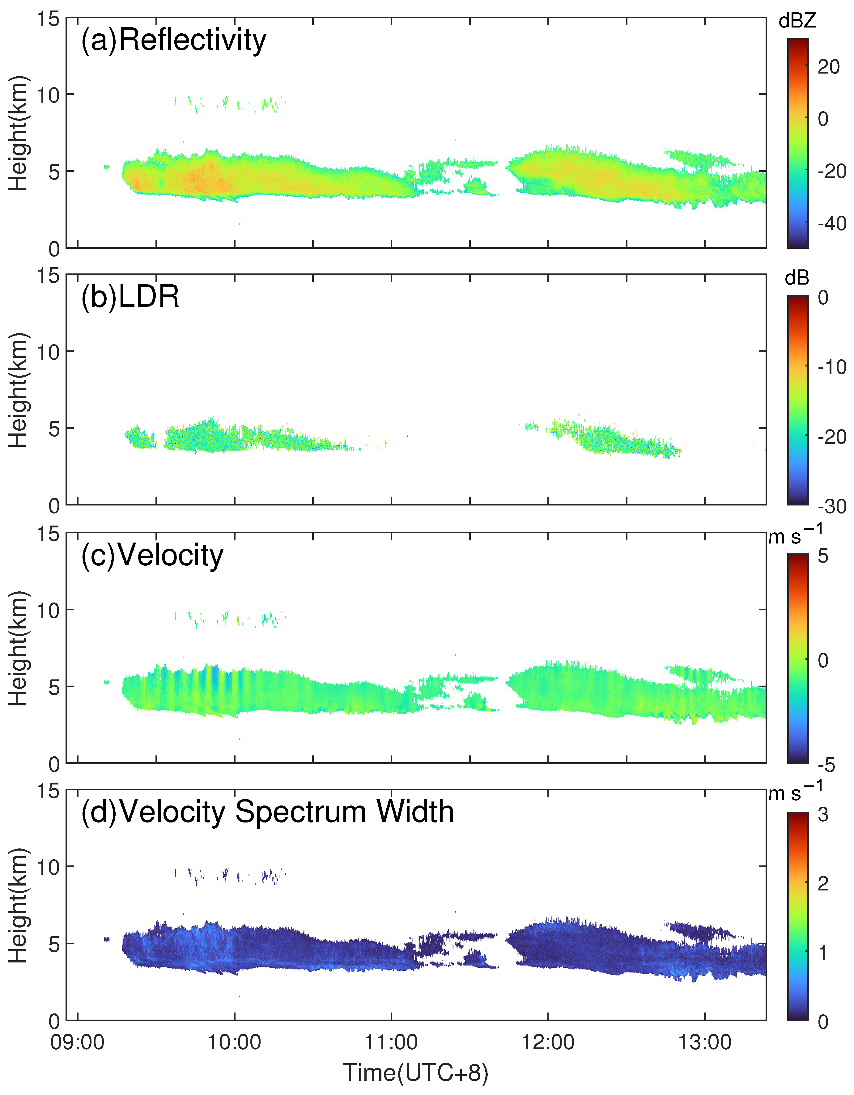
The basic data products of TJ-II, including reflectivity, LDR, velocity, and velocity spectrum width, can now be calculated based on the processed Doppler power spectrum. Figure 12 shows an example observed by TJ-II.
On this day, clouds were mainly concentrated in the middle distance of about 5 km. TJ-II clearly showed the change of reflectivity inside the cloud. At around 10:00, there were obvious repeated changes between positive and negative color strips in the velocity chart, indicating that there may be some convection. This was also evidenced by the wavy cloud top profiles at that time. There were sporadic bins near the 10 km and 10:00 areas that were not even detected by conventional algorithms, indicating that the TJ-II still suffers from lower peak power in detecting extremely weak cloud signals.
5. Conclusions and Future Work
The TJ-II is a dual-polarization solid-state pulse Doppler cloud radar. The birth of TJ-II stems from our dissatisfaction with TJ-I, the previous one with TWTA and dual antennas, in terms of size, lifetime, maintenance, etc. To address these issues, we developed TJ-II with SSPA and a single antenna. TJ-II utilizes pulse compression, segmented pulse, and dual PRF to overcome some of the limitations posed by the low power of the SSPA and high frequency of 94 GHz. Furthermore, a time-division receive channel is used to reduce costs. The digital signal source implemented by FPGA and DAC achieves the implementation of segmented waveform and dual PRF technique and facilitates future upgrades in waveform technology. The digital receiver module utilizes software-defined radio (SDR) technology to effectively reduce DC interference. Doppler spectrum processing methods are also optimized for weak cloud signals and scene adaptability, such as the half-folded phenomenon. The reduction in size and cost will help promote the deployment and use of the 94 GHz MMCRs. For example, it can be deployed on mobile platforms for localized monitoring of areas of significant activity. It can also be used to provide rapid support for extreme weather observations to gather more accurate data to support decision making.
TJ-II is still under development and optimization. Many works such as calibration and comparison measurements with other equipment (Ka-band radar, Lidar, etc.) are still in progress. In addition, long-term observations and feedback from radar users are needed to verify and optimize both software and hardware.
Author Contributions
H.L. designed the algorithm and wrote the paper under the guidance of J.G., H.L., J.W. and Z.C. were in charge of radar hardware design and observation experiments. J.G. was in charge of the whole project. All authors have read and agreed to the published version of the manuscript.
Funding
This research was funded by the National Natural Science Foundation of China (Grant No. 61671249) and the Jiangsu Innovation and Entrepreneurship Group Talents Plan.
Data Availability Statement
Data related to this article are available upon request to the corresponding author.
Conflicts of Interest
The authors declare no conflict of interest.
Appendix A
Appendix A.1. Deviation of the Ratio of the Mean to Standard Deviation of the Mixed Signal
In general, the mean and variance of a mixture of two random variables, such as noise and cloud signal, are given by
where is the proportion of the variable 1 in the mixture. and are the mean of noise and cloud signal, respectively. and are the standard deviation noise and cloud signal, respectively. When the variables follow the exponential distribution, where and , the Equation (A1) changes to Equation (A2).
In our application, noise is normalized to 1 by the noise level. Therefore, the Equation (A2) changes to Equation (A3):
The ratio of the mean to standard deviation in square format is given by Equation (A4):
Because , the ratio is always no greater than 1.
References
- Arking, A. The radiative effects of clouds and their impact on climate. Bull. Am. Meteorol. Soc. 1991, 72, 795–814. [Google Scholar] [CrossRef]
- Ran, Y.; Wang, H.; Tian, L.; Wu, J.; Li, X. Precipitation cloud identification based on faster-RCNN for Doppler weather radar. EURASIP J. Wirel. Commun. Netw. 2021, 2021, 19. [Google Scholar] [CrossRef]
- McGill, M.; Hlavka, D.; Hart, W.; Scott, V.S.; Spinhirne, J.; Schmid, B. Cloud physics lidar: Instrument description and initial measurement results. Appl. Opt. 2002, 41, 3725–3734. [Google Scholar] [CrossRef] [PubMed] [Green Version]
- Lhermitte, R. A 94-GHz Doppler radar for cloud observations. J. Atmos. Ocean. Technol. 1987, 4, 36–48. [Google Scholar] [CrossRef]
- Im, E.; Wu, C.; Durden, S.L. Cloud profiling radar for the CloudSat mission. In Proceedings of the IEEE International Radar Conference, Arlington, VA, USA, 9–12 May 2005; pp. 483–486. [Google Scholar] [CrossRef]
- Chandra, A.; Zhang, C.; Kollias, P.; Matrosov, S.; Szyrmer, W. Automated rain rate estimates using the Ka-band ARM zenith radar (KAZR). Atmos. Meas. Tech. 2015, 8, 3685–3699. [Google Scholar] [CrossRef] [Green Version]
- Takano, T.; Nakanishi, Y.; Takamura, T. High resolution FMCW Doppler radar FALCON-I for W-band meteorological observations. In Proceedings of the 2012 15 International Symposium on Antenna Technology and Applied Electromagnetics, Toulouse, France, 25–28 June 2012; pp. 1–4. [Google Scholar] [CrossRef]
- Huggard, P.; Oldfield, M.; Moyna, B.; Ellison, B.; Matheson, D.; Bennett, A.; Gaffard, C.; Oakley, T.; Nash, J. 94 GHz FMCW cloud radar. In Proceedings of the Millimetre Wave and Terahertz Sensors and Technology, Cardiff, UK, 15–18 September 2008; Volume 7117, pp. 16–21. [Google Scholar] [CrossRef]
- Wu, J.; Wei, M.; Hang, X.; Zhou, J.; Zhang, P.; Li, N. The first observed cloud echoes and microphysical parameter retrievals by China’s 94-GHz cloud radar. J. Meteorol. Res. 2014, 28, 430–443. [Google Scholar] [CrossRef]
- Delanoë, J.; Protat, A.; Vinson, J.P.; Brett, W.; Caudoux, C.; Bertrand, F.; Du Châtelet, J.P.; Hallali, R.; Barthes, L.; Haeffelin, M.; et al. BASTA: A 95-GHz FMCW Doppler radar for cloud and fog studies. J. Atmos. Ocean. Technol. 2016, 33, 1023–1038. [Google Scholar] [CrossRef] [Green Version]
- Montgomery, R.; Courtney, P. Solid-State PAs Battle TWTAs for ECM Systems. Microw. J. 2017. Available online: https://www.microwavejournal.com/articles/28478-solid-state-pas-battle-twtas-for-ecm-systems (accessed on 10 May 2023).
- Wang, J.; Lin, H.; Yang, F.; Xu, G.; Ge, J. Design of 94 GHz Dual-Polarization Antenna Fed by Diagonal Horn for Cloud Radars. IEEE Access 2022, 10, 22480–22486. [Google Scholar] [CrossRef]
- Hildebrand, P.H.; Sekhon, R. Objective determination of the noise level in Doppler spectra. J. Appl. Meteorol. (1962–1982) 1974, 13, 808–811. [Google Scholar] [CrossRef]
- Petitdidier, M.; Sy, A.; Garrouste, A.; Delcourt, J. Statistical characteristics of the noise power spectral density in UHF and VHF wind profilers. Radio Sci. 1997, 32, 1229–1247. [Google Scholar] [CrossRef]
- Shupe, M.D.; Kollias, P.; Matrosov, S.Y.; Schneider, T.L. Deriving mixed-phase cloud properties from Doppler radar spectra. J. Atmos. Ocean. Technol. 2004, 21, 660–670. [Google Scholar] [CrossRef]
- Yuan, Y.; Di, H.; Liu, Y.; Yang, T.; Li, Q.; Yan, Q.; Xin, W.; Li, S.; Hua, D. Detection and analysis of cloud boundary in Xi’an, China, employing 35 GHz cloud radar aided by 1064 nm lidar. Atmos. Meas. Tech. 2022, 15, 4989–5006. [Google Scholar] [CrossRef]
- Maahn, M.; Kollias, P. Improved Micro Rain Radar snow measurements using Doppler spectra post-processing. Atmos. Meas. Tech. 2012, 5, 2661–2673. [Google Scholar] [CrossRef] [Green Version]
- Zheng, J.F.; Liu, L.P.; Zeng, Z.M.; Xie, X.; Wu, J.; Feng, K. Ka-band millimeter wave cloud radar data quality control. J. Infrared Millim. Waves 2016, 35, 748–757. [Google Scholar]
- Joe, P.; May, P. Correction of dual PRF velocity errors for operational Doppler weather radars. J. Atmos. Ocean. Technol. 2003, 20, 429–442. [Google Scholar] [CrossRef]
- Torres, S.M.; Dubel, Y.F.; Zrnić, D.S. Design, implementation, and demonstration of a staggered PRT algorithm for the WSR-88D. J. Atmos. Ocean. Technol. 2004, 21, 1389–1399. [Google Scholar] [CrossRef]
Figure 1.
The TJ-II cloud radar.
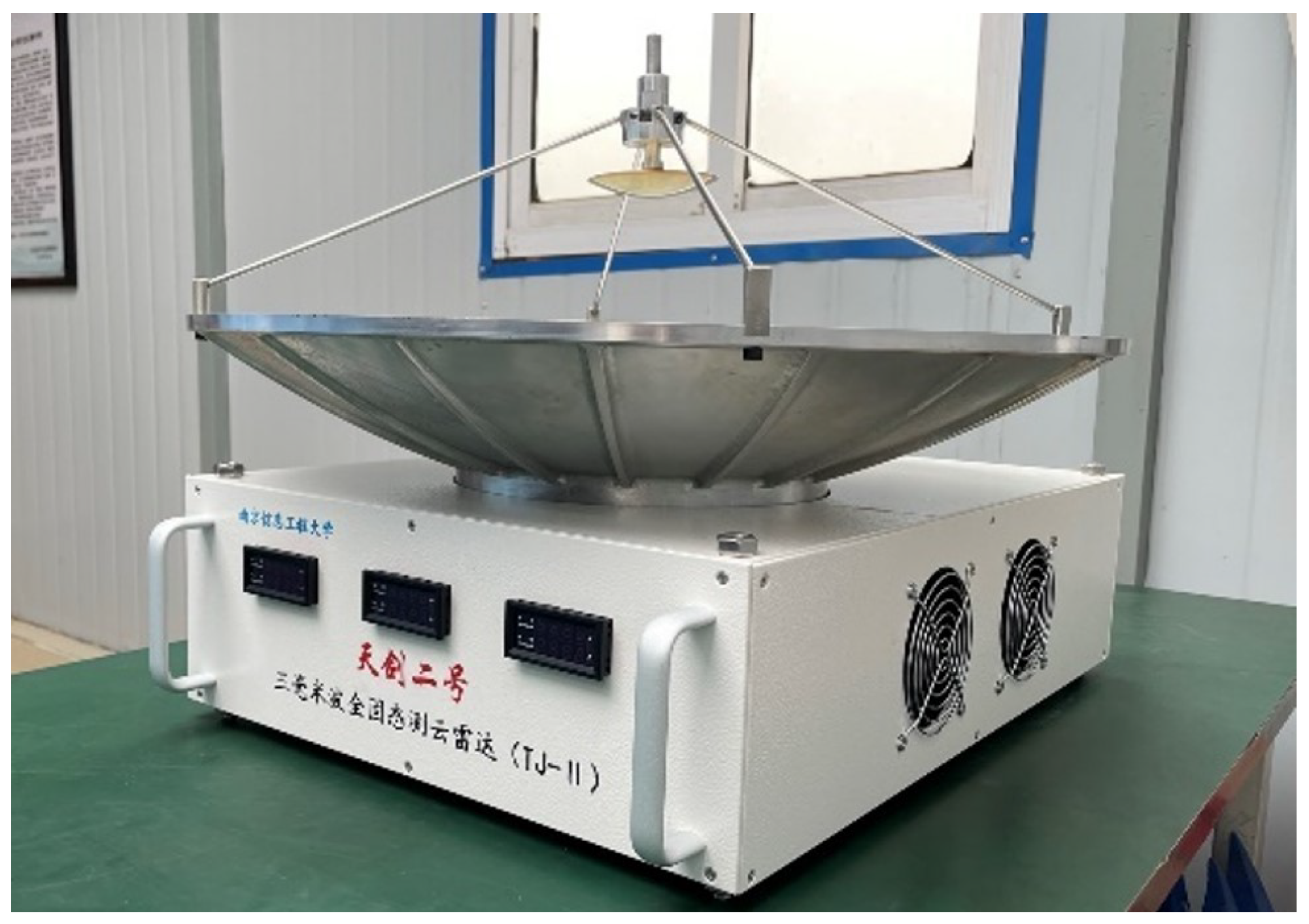
Figure 2.
Design consideration of TJ-II system form.
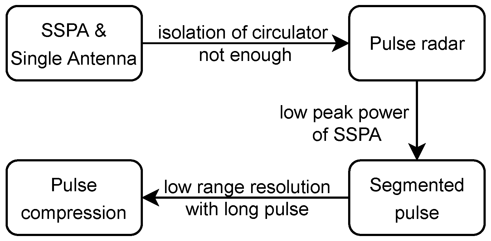
Figure 3.
Two types of segmented pulse.
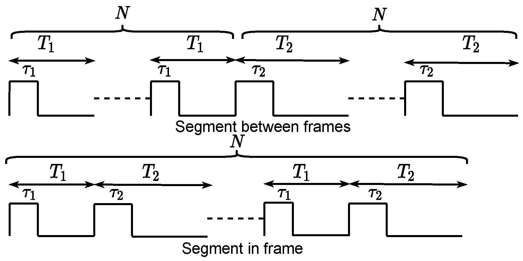
Figure 4.
Block diagram of RF front end.
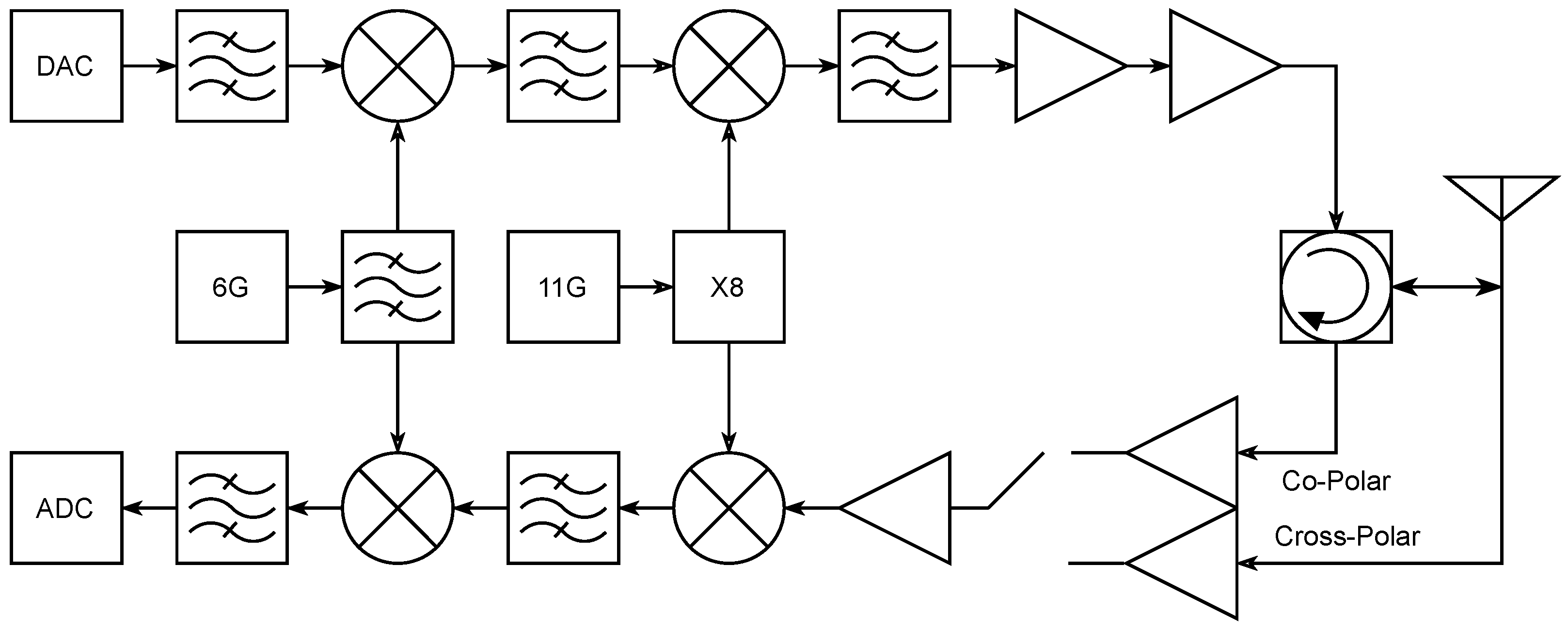
Figure 5.
(a) Photograph of the feed and (b) assembled on the deep of the main reflector. (c) Photograph of the antenna system tested in a microwave anechoic chamber.
Figure 5.
(a) Photograph of the feed and (b) assembled on the deep of the main reflector. (c) Photograph of the antenna system tested in a microwave anechoic chamber.
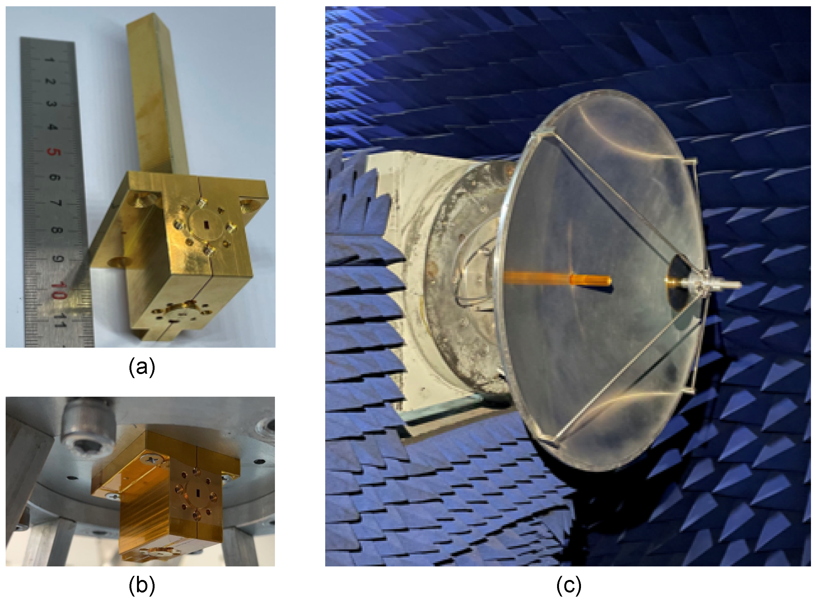
Figure 6.
Example of the effect of noise level estimation bias on weak signals. (a) Raw power spectrum (b) cloud signal mask result with noise level estimated by our method (c) cloud signal mask result with noise level 1 dB higher than (b).
Figure 6.
Example of the effect of noise level estimation bias on weak signals. (a) Raw power spectrum (b) cloud signal mask result with noise level estimated by our method (c) cloud signal mask result with noise level 1 dB higher than (b).
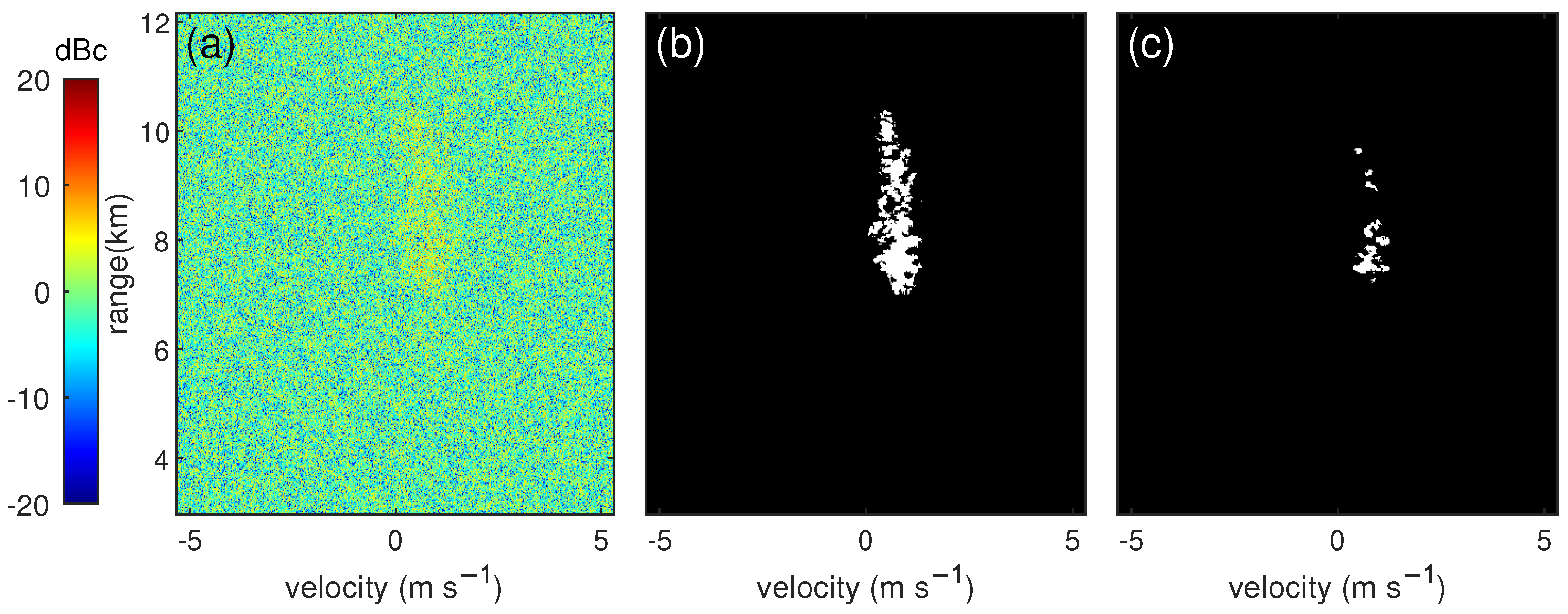
Figure 7.
Subregion division.

Figure 8.
Ratio of the mean to standard deviation of the mixed signal.

Figure 9.
Example of cloud detection process. (a) is the raw power spectrum. (b) is the mask result of pre-mask processing. (c,d) are the mask results of step two processing with iteration times 1 and 5, respectively.
Figure 9.
Example of cloud detection process. (a) is the raw power spectrum. (b) is the mask result of pre-mask processing. (c,d) are the mask results of step two processing with iteration times 1 and 5, respectively.

Figure 10.
Example of the half-folded phenomenon. (a,b) is the mask result by cloud signal detection processing with PRT 150 us and 100 us, respectively.
Figure 10.
Example of the half-folded phenomenon. (a,b) is the mask result by cloud signal detection processing with PRT 150 us and 100 us, respectively.

Figure 11.
Some cases of half-folded state. (a) Normal case, (b) case with ultra-wide spectral width, and (c) case with sub-peak.
Figure 11.
Some cases of half-folded state. (a) Normal case, (b) case with ultra-wide spectral width, and (c) case with sub-peak.

Figure 12.
Example data products observed on 17 November 2021.

Table 1.
Basic parameters of TJ-II.
| Frequency | 94 GHz |
| Transmitter type | Solid-state power amplifier |
| Peak transmit power | 6 W |
| Antenna type | Cassegrain antenna |
| Antenna gain | 50.85 dB |
| 3 dB Beamwidth | 0.45° |
| Detection range | 0.3 to 15 km |
| Range resolution | 15 m |
| Pulse length | 1.5/5/20 us |
| Pulse repetition time | 120/150 us |
| FFT numbers | 512 |
| Sensitivity | −30 to 50 dBZ |
Disclaimer/Publisher’s Note: The statements, opinions and data contained in all publications are solely those of the individual author(s) and contributor(s) and not of MDPI and/or the editor(s). MDPI and/or the editor(s) disclaim responsibility for any injury to people or property resulting from any ideas, methods, instructions or products referred to in the content. |
© 2023 by the authors. Licensee MDPI, Basel, Switzerland. This article is an open access article distributed under the terms and conditions of the Creative Commons Attribution (CC BY) license (https://creativecommons.org/licenses/by/4.0/).
Share and Cite
MDPI and ACS Style
Lin, H.; Wang, J.; Chen, Z.; Ge, J. A 94 GHz Pulse Doppler Solid-State Millimeter-Wave Cloud Radar. Remote Sens. 2023, 15, 3098. https://doi.org/10.3390/rs15123098
AMA Style
Lin H, Wang J, Chen Z, Ge J. A 94 GHz Pulse Doppler Solid-State Millimeter-Wave Cloud Radar. Remote Sensing. 2023; 15(12):3098. https://doi.org/10.3390/rs15123098
Chicago/Turabian StyleLin, Hai, Jie Wang, Zhenhua Chen, and Junxiang Ge. 2023. "A 94 GHz Pulse Doppler Solid-State Millimeter-Wave Cloud Radar" Remote Sensing 15, no. 12: 3098. https://doi.org/10.3390/rs15123098
Note that from the first issue of 2016, this journal uses article numbers instead of page numbers. See further details here.