Algorithm for the Reconstruction of the Ground Surface Reflectance in the Visible and Near IR Ranges from MODIS Satellite Data with Allowance for the Influence of Ground Surface Inhomogeneity on the Adjacency Effect and of Multiple Radiation Reflection

Abstract

An atmospheric correction algorithm is proposed for the reconstruction of the ground surface reflectance from the data of satellite measurements. A distinctive feature of the algorithm is that it takes into account the influence of the ground surface inhomogeneity on the adjacency effect and additional illumination of the ground surface by reflected radiation. These factors are important for the reconstruction of the reflectance of ground surface fragments with sharp reflectance changes and high atmospheric turbidity. The algorithm is based on Monte Carlo programs developed by the authors. To reduce the computing time, we have proposed some original criteria and approaches. To estimate the capabilities of the developed algorithm, its results have been validated by comparing with the results of the MOD09 algorithm for four MODIS bands and measurements for the Portugal surface fragment with coordinates 38.829 N, 8.791 W. Good agreement of the results obtained by the proposed algorithm with the surface measurements and the data obtained by the MOD09 algorithm demonstrates the efficiency of the proposed algorithm in the reconstruction of the ground surface reflectance.

1. Introduction

Algorithms for retrieving the ground surface reflectance from satellite measurements have been developed for more than four decades, starting from such studies as [1]. To date, there are dozens of ways for solving this problem. The algorithms based on the solution of the radiative transfer equation (RTE) are referred to as radiative transfer model (RTM) algorithms. Algorithms are developed for satellite sensing of both land and water surfaces. The material presented below is primarily related to the problem of land sensing under conditions of a cloudless atmosphere. The problem solution for the water surface has its own specificity. The reflection from water surfaces is considered specular, in contrast to most land surfaces. According to [2], the received radiance in ocean remote sensing consists of: (1) radiation that did not interact with the water surface, (2) specularly reflected solar radiation, (3) radiation reflected by foam and whitecaps, and (4) radiation scattered by the upper water layer. Water surfaces are horizontally more uniform than land areas. Therefore, water surface can be treated as horizontally uniform when inverse problems of sensing are solved. In general, the state-of-the-art in algorithms for sensing of water surfaces can be judged from [2,3,4,5]. According to [6], a signal received by a satellite receiver in the visible and near-IR ranges can be divided into the following components (Figure 1): (1) radiation that does not interact with the ground surface (Figure 1a), (2) direct solar radiation that interacts with the surface fragment under study (Figure 1b), (3) diffuse solar radiation that interacts with the surface fragment under study (Figure 1c), (4) adjacency effect (AE) due to single reflected radiation (Figure 1d), and (5) adjacency effect due to multiple reflected radiation (Figure 1e).

However, the solution of the system of equations without additional simplifications is very time-consuming. Thus, this approach is hard to apply to actual satellite data. That is why similar problems in later studies were solved with some simplifications reducing the computer time needed to obtain the desired solutions. RTM algorithms differ in the way of considering the following factors: (1) non-Lambertian character of the surface, (2) adjacency effect, (3) multiple reflection, (4) absorption, (5) radiation polarization, and (6) surface topography.

Table 1. RTM algorithms for retrieval of the surface reflectance.

Factor	Authors/Reference
	Putsay	Tanre	Berk	Vermote	Lyapustin	Reinersman	Katkovskiy	Shi
	[7]	[6]	[8]	[9]	[10]	[11]	[12]	[13]
Surface		Non-		Non-	Non-			Non-
model	Lamb	Lamb	Lamb	Lamb	Lamb	Lamb	Lamb	Lamb
Adjacency
effect	accurate	accurate	approx.	approx.	accurate	accurate	approx.	approx.
Multiple
reflection	No	approx.	approx.	approx.	approx.	approx.	approx.	approx.
Molecular
absorption	accurate	accurate	accurate	accurate	accurate	accurate	approx.	accurate
Polarization	No	No	No	Yes	Yes	No	No	No
Topography	No	No	No	No	No	No	No	Yes

compares some RTM algorithms for retrieval of the surface reflectance considering/ignoring the factors affecting the radiative transfer.

It can be seen from Table 1 that some algorithms employ the approximate Lambertian surface model, while others consider accurately the non-Lambertian character of the surface, usually, after the solution of the problem in the Lambertian approximation. Many algorithms take into account the adjacency effect approximately. They assume that the point spread function (PSF) of the AE is axisymmetric or that the surface around an observed pixel is uniform. For example, it is shown in p. 34 of [9] that PSF of the AE is significantly non-axisymmetric in azimuth if the optical axis of the receiver system is tilted by 70º about nadir. All the studies analyzed in Table 1 either ignore the multiple reflection or assume that the surface around the observed pixel is uniform. However, it is stated in some papers (for example, in [14]) that the consideration of multiple reflection may be important for situations of a sharp transition from a low reflective surface to a high reflective surface. In some papers, molecular absorption is taken into account separately from scattering, which may be unacceptable in the case of a significant influence of multiple scattering. The radiation polarization is also ignored in many studies. However, for example, our estimates in [15] have shown that this factor may be important for the solution of the inverse problem under consideration. According to [16], ignoring the effects of polarization leads to the following errors in calculated top-of-atmosphere reflectances: more than 10% for a molecular atmosphere and up to 5% for an aerosol atmosphere. If there is a large height difference in the observed surface, then topography can also be an important factor affecting the results of solution. Most papers considering topography ignore the radiation extinction and the adjacency effect. It should be emphasized that, in a cloudy atmosphere, it is often unacceptable to ignore the adjacency effect from clouds in approaches to the interpretation of the data of passive satellite sensing of the ground surface under the conditions of a cloudless atmosphere that are described in [6,7,8,9,10,11,12,13]. The adjacency effect from clouds is studied, for example, in [17,18,19,20,21]. The algorithms considered in Table 1 and similar ones have formed the basis for several software packages: ATCOR [22], ACORN [23], ATREM [24], FLAASH [25], HATCH [26], and others. Nevertheless, the problem of correct estimation of surface reflectance from satellite data is not completely solved yet.

In [27], we have proposed the algorithm for retrieving the ground surface reflectances observed through the cloudless atmosphere. This algorithm allows accurate consideration of the adjacency effect, multiple reflection of the radiation from the surface, and the radiation polarization. In this paper, this algorithm is validated against the MODIS data and the ground-based measurements in Portugal [28]. The results obtained with our algorithm are compared with the MOD09 results.

2. Algorithm for Retrieval of the Surface Reflectance

2.1. Assumptions and Problem Formulation

When developing the algorithm for retrieval of surface reflectance $r_{surf}$, we have assumed the following:

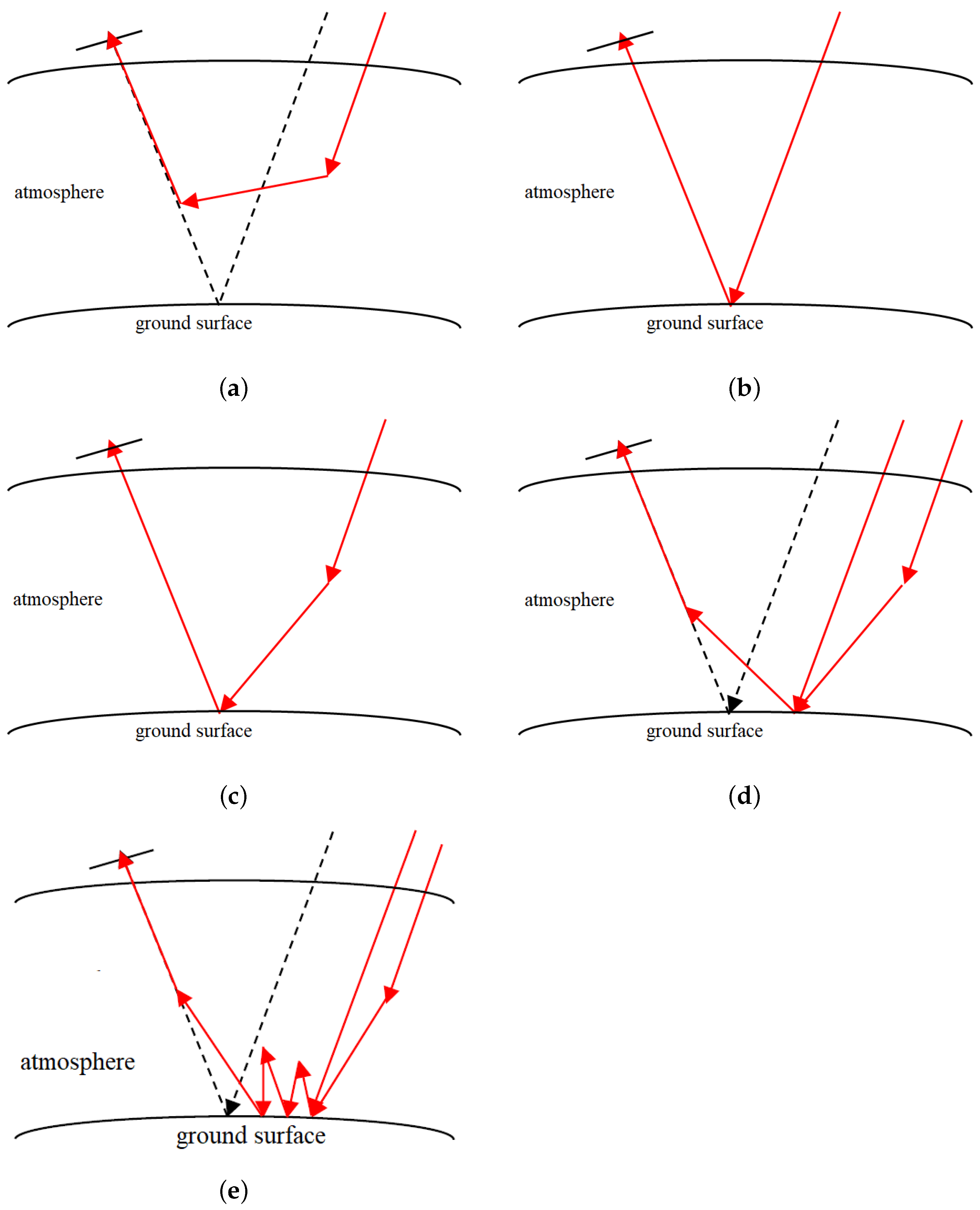
• The atmosphere is a scattering and absorbing aerosol-gas medium.
• The atmosphere is cloudless and vertically stratified into 32 uniform layers.
• The “atmosphere-ground surface” system is spherical, and refraction is ignored. The boundaries of the atmospheric layers are spheres.
• The source of radiation is the sun. There are no other sources.
• The ground surface is non-uniform and reflects radiation according to the Lambert law.
• The ground surface is uniform within a pixel.
• Local topography is ignored.
• The change in the illumination of the ground surface due to a change in the solar zenith angle is negligibly small.
• The radiative transfer is considered in the monochromatic approximation.

According to the algorithm [29], the non-Lambertian character of the ground surface can be taken into account once the ground surface reflectances $r_{surf}$ are determined in the approximation of Lambertian reflection. The most common way to take into account the non-Lambertian character of the surface is by using the Ross–Thick–Li–Spars model [30]. Alternative BRDF models were presented in works [31,32,33,34,35]. The analysis of earlier publications shows that the simultaneous consideration of surface topography and reflection inhomogeneity was not performed in the solution of the inverse problem. Knowing surface slopes (from, for example, Ref. [36]), we can normalize the surface before performing the atmospheric correction or use corrections for surface topography in the systems of equations to be solved.

Let the task be to determine surface reflectances for the considered fragment of the ground surface from radiance measured by a satellite receiver.

2.2. System of Equations to Be Solved

In the above assumptions, the algorithm is based on the decomposition of the radiance measured by a satellite receiver into the following components:

$$\begin{array}{c}{I}_r({\phi }_{N,ij},{\lambda }_{N,ij},{\mu }_{sun},{\mu }_{d,ij},{\alpha }_{ij})=I_{atm}({\mu }_{sun},{\mu }_{d,ij},{\alpha }_{ij})\hfill \\ \hfill +I_0({\phi }_{N,ij},{\lambda }_{N,ij},{\mu }_{sun},{\mu }_{d,ij})+I_{surf,sc}({\phi }_{N,ij},{\lambda }_{N,ij},{\mu }_{sun},{\mu }_{d,ij})\end{array}$$

(1)

where $I_{atm}$ is the radiance of the flux non-interacting with the ground surface (Figure 1a); $I_0$ is the radiance of the flux reflected from the surface that reached the receiver without scattering upon the reflection (Figure 1b,c); $I_{surf,sc}$ is the radiance of the flux reflected from the ground surface that reached the receiver after scattering (Figure 1d,e); ${\phi }_{N,ij}$, ${\lambda }_{N,ij}$ are the coordinates of the center of the observed pixel in the i-th line and j-th column of the considered fragment; ${\mu }_{sun}$ is the cosine of the solar zenith angle; ${\mu }_d$ is the cosine of the zenith angle of the receiving system; and $\alpha$ is the relative azimuth angle between the directions to the satellite and to the sun at the observed surface point.

Within the framework of the above assumptions, the value of $I_0$ can be found as

$$I_0({\phi }_{N,ij},{\lambda }_{N,ij},{\mu }_{sun},{\mu }_{d,ij})=r_{surf}({\phi }_{N,ij},{\lambda }_{N,ij})E_{sum}({\phi }_{N,ij},{\lambda }_{N,ij},{\mu }_{sun})\frac{1}{\pi }exp(-\tau \left({\mu }_{d,ij}\right)),$$

(2)

where $E_{sum}$ is the total irradiance at the surface point and $\tau$ is the optical thickness of the path from the observed surface point to the receiver.

In the above assumptions, the value of $I_{surf,sc}$ can be determined as

$$\begin{array}{c}{I}_{surf,sc}({\phi }_{N,ij},{\lambda }_{N,ij},{\mu }_{sun},{\mu }_{d,ij})\hfill \\ =\sum _{k=1}^{N_i}\sum _{l=1}^{N_j}{r}_{surf}({\phi }_{N,kl},{\lambda }_{N,kl})E_{sum}({\phi }_{N,kl},{\lambda }_{N,kl},{\mu }_{sun})h({\rho }_{w,ijkl},{\alpha }_{w,ijkl},{\mu }_{d,ij})S_{kl}\\ \hfill +\overline{Q}{A}_{out}({\phi }_{N,ij},{\lambda }_{N,ij}),\end{array}$$

(3)

$$A_{out}({\phi }_{N,ij},{\lambda }_{N,ij})={\int \int }_{S}h({\rho }_w,{\alpha }_w,{\mu }_{d,ij})dS-\sum _{k=1}^{N_i}\sum _{l=1}^{N_j}h({\rho }_{w,ijkl},{\alpha }_{w,ijkl},{\mu }_{d,ij})S_{kl}$$

(4)

where $S_{kl}$ is the area of the pixel in the k-th line and l-th column of the considered fragment; ${\rho }_{w,ijkl}$ is the distance from the point with coordinates ${\phi }_{N,ij}$, ${\lambda }_{N,ij}$ to the point with coordinates ${\phi }_{N,kl}$, ${\lambda }_{N,kl}$ along the earth’s surface; ${\alpha }_{w,ijkl}$ is the relative azimuthal angle at the point with coordinates ${\phi }_{N,ij}$, ${\lambda }_{N,ij}$ between the direction to the receiving system and to the point with coordinates ${\phi }_{N,kl}$, ${\lambda }_{N,kl}$; ${\rho }_w$, ${\alpha }_w$ are the surface polar coordinates on the spherical ground surface from the observed point; h is PSF of the AE, 1/(m${}^2$ sr); $dS$ is the differential over the ground surface; and $\overline{Q}$ the average luminosity of the considered surface fragment in the approximation of the uniform surface, W/(m${}^2$ $\mathsf{\mu }$m). The first term on the right side in the Equation (3) estimates the adjacency effect from the considered area of the ground surface. The second term on the right side in the Equation (3) estimates the adjacency effect from regions outside the considered area of the ground surface.

It is proposed to determine the total irradiance of the ground surface $E_{sum}$ with allowance for the additional irradiance due to multiple reflected radiation by the following equation:

$$\begin{array}{c}{E}_{sum}({\phi }_{N,ij},{\lambda }_{N,ij},{\mu }_{sun})=E_0\left({\mu }_{sun}\right)+E_0\left({\mu }_{sun}\right)\sum _{k=1}^{N_i}\sum _{l=1}^{N_j}{r}_{surf}({\phi }_{N,kl},{\lambda }_{N,kl})h_1\left({\rho }_{w,ijkl}\right)S_{kl}\hfill \\ \hfill +C_{out}({\phi }_{N,ij},{\lambda }_{N,ij})\overline{r_{surf}}+E_0\left({\mu }_{sun}\right)\frac{\overline{(r_{surf}}{\gamma }_1{)}^2}{1-\overline{r_{surf}}{\gamma }_1}\end{array}$$

(5)

$$C_{out}({\phi }_{N,ij},{\lambda }_{N,ij})={\gamma }_1-\sum _{k=1}^{N_i}\sum _{l=1}^{N_j}{h}_1\left({\rho }_{w,ijkl}\right)S_{kl}$$

(6)

$${\gamma }_1\equiv 2\pi \underset{0}{\overset{\pi R_e}{\int }}{h}_1\left({\rho }_w\right)d{\rho }_w$$

where $E_0$ is the irradiance of the ground surface for a non-reflective ground surface, W/(m${}^2$ $\mathsf{\mu }$m); $h_1$ is PSF of the additional surface irradiance formation, 1/m${}^2$; ${\gamma }_1$ is the integral of the function $h_1$ over the entire ground surface; $d{\rho }_w$ is the differential of the distance over the spherical ground surface; and $R_e$ is the Earth radius. The first term on the right side of the Equation (5) characterizes the irradiance of the ground surface by non-reflected radiation. The second term describes additional irradiance by radiation singly reflected from the points of the area under consideration. The third term gives the additional irradiance by radiation singly reflected outside the area under consideration. The fourth term describes the additional irradiance by reflected radiation with a reflection multiplicity of two or more.

Most alternative algorithms for retrieval of surface reflectance (for example, [9,10]) employ the simplified equation

$$E_{sum}({\phi }_{N,ij},{\lambda }_{N,ij},{\mu }_{sun})=\frac{E_0\left({\mu }_{sun}\right)}{1-\overline{r_{surf}}{\gamma }_1}$$

(7)

in place of Equation (5). In Equation (7), $\overline{r_{surf}}$ is the reflectance averaged over the observed surface fragment in the approximation of the uniform surface.

According to our calculations, the upper estimate of the error of using Equation (7) is ${\Delta }_1=\frac{r_{surf,max}{\gamma }_1}{1-r_{surf,max}{\gamma }_1}$, while that for Equation (5) is ${\Delta }_2=\frac{{\left(r_{surf,max}{\gamma }_1\right)}^2}{1-r_{surf,max}{\gamma }_1}$, ($r_{surf,max}$ is the maximal value of the surface reflectance over the considered surface fragment). For example, for the situation $r_{surf}<0.4$, we have obtained ${\Delta }_1\le 0.106$ and ${\Delta }_2\le 0.01$ for the molecular atmosphere in the visible wavelength range and ${\Delta }_1\le 0.19$ and ${\Delta }_2\le 0.03$ for the high atmospheric turbidity (${AOD}_{0.55}=7.0$). Thus, in the limiting situations, the use of Equation (7) may yield an unacceptably high error (up to 19% of the total surface irradiance). At the same time, the consideration of the inhomogeneity of surface reflection in the double reflected radiation allows this error to be decreased down to below 3%. A description of how this assessment was made has been added to the Supplementary Materials [37].

With allowance for Equations (1)–(5), the solution of the problem is divided into two stages:

(1) Determination of the surface luminosity $Q=r_{surf}{E}_{sum}$ from the system of linear equations

$$\begin{array}{c}{I}_r({\phi }_{N,ij},{\lambda }_{N,ij},{\mu }_{sun},{\mu }_{d,ij},{\alpha }_{ij})-I_{atm}({\mu }_{sun},{\mu }_{d,ij},{\alpha }_{ij})=Q({\phi }_{N,ij},{\lambda }_{N,ij},{\mu }_{sun})\frac{1}{\pi }exp(-\tau \left({\mu }_{d,ij}\right))\hfill \\ \hfill +\sum _{k=1}^{N_i}\sum _{l=1}^{N_j}Q({\phi }_{N,kl},{\lambda }_{N,kl},{\mu }_{sun})h({\rho }_{w,ijkl},{\alpha }_{w,ijkl},{\mu }_{d,ij})S_{kl}+\overline{Q}{A}_{out}({\phi }_{N,ij},{\lambda }_{N,ij})\end{array}$$

(8)

(2) Determination of the surface reflectance from the system of nonlinear equations

$$\begin{array}{c}Q({\phi }_{N,ij},{\lambda }_{N,ij},{\mu }_{sun})=r_{surf}({\phi }_{N,ij},{\lambda }_{N,ij})E_0\left({\mu }_{sun}\right)\hfill \\ \times (1+\sum _{k=1}^{N_i}\sum _{l=1}^{N_j}{r}_{surf}({\phi }_{N,kl},{\lambda }_{N,kl})h_1\left({\rho }_{w,ijkl}\right)S_{kl}\\ \hfill +C_{out}({\phi }_{N,ij},{\lambda }_{N,ij})\overline{r_{surf}}+\frac{{\left(\overline{r_{surf}}{\gamma }_1\right)}^2}{1-\overline{r_{surf}}{\gamma }_1})\end{array}$$

(9)

In general, the above Equations (1)–(3) are similar, with the exception of some minor details, to the equations from works [6,7,8,9,10,11,12,13]. The closest approach is in [11]. Equation (5), used in the present algorithm, is usually not used. Instead, Equation (7) is most often used. Moreover, several additional simplifications to reduce the computational time are considered below.

2.3. Additional Simplifications to Reduce the Computation Time

Systems of Equations (8) and (9) have the following features: (i) if the functions h and $h_1$ are calculated separately for every pixel, then the computation takes a huge time for a large surface fragment (hundreds of thousands of pixels or more), (ii) summation over all image lines and columns yields the systems with constants having the dimension of $(N_i$×$N_j{)}^2$, which makes systems (8) and (9) of little use, (iii) the calculation of $I_{atm}$ for every pixel also takes a lot of computing time, (iv) pixels may be arranged unevenly over the ground surface—therefore, an algorithm is needed to determine quickly the areas of fragments closest to the center of a given pixel $S_{kl}$. To solve these problems, we have proposed some methods [27,38] that are described below.

2.3.1. Use of Isoplanar Zones

To avoid calculation of h for every pixel separately, it is proposed to divide the surface fragment, for which the reflectances are retrieved, into zones, within which the function h can be considered constant in the variable ${\mu }_d$ with some given error $\delta$. It is obvious that the function h is the same at the fixed angle ${\theta }_d$ of deviation from the nadir direction and the arbitrary azimuth angle. Therefore, isoplanar zones (zones, where h is the same) should be limited to rings with some constant angles of deviation from the nadir direction. Alternative algorithms (e.g., Ref. [9]) often use the axisymmetric function h obtained in nadir observations instead. To set the boundaries of isoplanar zones, we propose to use the recurrent equation [38]:

$$\left\{\begin{array}{c}\hfill H\left({\mu }_k\right)=H\left(1\right)-C{(1-{\mu }_k)}^N\\ \hfill {\mu }_{k+1}=1-{\left[\frac{1}{C}\left(H\left(1\right)-\frac{H\left({\mu }_k\right)}{1+\delta }\right)\right]}^{1/N}\end{array}\right.$$

(10)

$$H\left({\mu }_k\right)\equiv \frac{1}{\pi }exp(-\tau \left({\mu }_k\right))+{\int \int }_{S}h({\rho }_w,{\alpha }_w,{\mu }_k)dS$$

(11)

$${\mu }_k\equiv cos{\theta }_k$$

The use of Equation (10) is justified in the Supplementary Materials [37].

2.3.2. Use of the Adjacency Effect Radius

The system of Equation (8) includes the terms responsible for the adjacency effect (AE) from all zones of the observed surface fragment. However, PSF of the AE is a rapidly decreasing function. Therefore, for any h, we can set (with some error) the AE radius $R_k$, outside which the adjacency effect can be considered equal to 0. Each isoplanar zone has its own radius $R_k$. We set $R_k$ so that the approximate surface luminosity $\tilde{Q}$ differs from the exact value of Q by smaller than the preset discrepancy ${\delta }_1$, that is,

$$1\ge mi{n}_{i,j}\frac{Q_{ij}}{\widetilde{Q_{ij}}}\ge {\delta }_1.$$

(12)

Condition (12) is based on the fact that summation of only terms within $R_k$ in Equation (8) overestimates the value of Q. It can be shown that, to fulfill condition (12), it is sufficient to fulfill the condition on the AE radius $R_k$:

$$k_1\left(R_k\right)\equiv \frac{{\int \int }_{S\left(R_k\right)}h({\rho }_w,{\alpha }_w,{\mu }_k)dS}{{\int \int }_{S}h({\rho }_w,{\alpha }_w,{\mu }_k)dS}\ge {\delta }_1+({\delta }_1-1)\frac{\frac{1}{\pi }exp(-\tau \left({\mu }_k\right))}{{\int \int }_{S}h({\rho }_w,{\alpha }_w,{\mu }_k)dS},$$

(13)

where $S\left(R_k\right)$ is the region on a spherical earth’s surface bounded by a radius $R_k$. The use of Equation (13) is justified in the Supplementary Materials [37].

Then, with known $R_k$, for each isoplanar zone, for any pixel we can find the range of lines k and columns l limiting the AE radius. Alternative algorithms considering the adjacency effect (for example, [9]) often use the fixed number of lines and columns for all situations, which ignores the dependence of $R_k$ on the state of the atmosphere and ${\mu }_d$.

2.3.3. Use of the Radius of Effect of Single Reflection on Ground Surface Illumination

In the sums over k and l in nonlinear system of Equation (9), we propose to remain only terms inside the radius of formation of additional irradiance $R_S$. To set $R_S$, we impose the condition that the error in determining $r_{surf}$ does not exceed ${\delta }_2$:

$$1\ge \underset{i,j}{min}\frac{r_{surf,ij}}{{\tilde{r}}_{surf,ij}}\ge {\delta }_2.$$

(14)

Condition (14) is reasoned by the fact that the use of $R_S$ overestimates $r_{surf}$. It can be shown (Supplementary Materials [37]) that, for condition (14) to be true, it is sufficient to satisfy the following condition:

$$k_2\left(R_S\right)\equiv \frac{2\pi {\int }_0^{R_S}{h}_1\left({\rho }_w\right)d{\rho }_w}{{\gamma }_1}\ge \frac{{\delta }_2}{{\gamma }_1}(\frac{{\delta }_2}{1-{\gamma }_1}-1),$$

(15)

Then, with known $R_S$, for each pixel we can find the range of lines k and columns l limiting the radius of formation of additional irradiance.

2.3.4. Use of Approximations for $I_{atm}$

The value of $I_{atm}$ depends on three variables characterizing the mutual position of the sun and the receiver ${\mu }_{sun},{\mu }_d$ and $\alpha$. If the surface fragment, for which atmospheric correction is performed, is small, then $I_{atm}$ can be considered as approximately constant. Otherwise, instead of calculating this value for each location of the receiver and the sun, it is proposed to use the approximation formula

$$I_{atm}({\mu }_{sun},{\mu }_d,\alpha )=-\frac{B({\mu }_d,\alpha )+\sqrt{B{({\mu }_d,\alpha )}^2-4A({\mu }_d,\alpha )C_{13}}}{2A({\mu }_d,\alpha ){\mu }_d},$$

(16)

$$A({\mu }_d,\alpha )=\left\{\begin{array}{c}\hfill C_{11}{\mu }_d^2+C_{21}{\left(\sqrt{1-{\mu }_d^2}cos\alpha \right)}^2+C_{22}{\mu }_d\sqrt{1-{\mu }_d^2}cos\alpha -{\left(\sqrt{1-{\mu }_d^2}sin\alpha \right)}^2,\alpha \le {90}^{°}\\ \hfill C_{11}{\mu }_d^2+C_{31}{\left(\sqrt{1-{\mu }_d^2}cos\alpha \right)}^2+C_{32}{\mu }_d\sqrt{1-{\mu }_d^2}cos\alpha -{\left(\sqrt{1-{\mu }_d^2}sin\alpha \right)}^2,\alpha >{90}^{°}\end{array}\right.$$

(17)

$$B({\mu }_d,\alpha )=\left\{\begin{array}{c}\hfill C_{12}{\mu }_d+C_{23}\sqrt{1-{\mu }_d^2}cos\alpha ,\alpha \le {90}^{°}\\ \hfill C_{12}{\mu }_d+C_{33}\sqrt{1-{\mu }_d^2}cos\alpha ,\alpha >{90}^{°}\end{array}\right.$$

(18)

where $C_{11},C_{12},C_{13},C_{21},C_{22},C_{23},C_{31},C_{32},C_{33}$ are the approximation constants. The approximation constants are determined by the least-square fit method from the values of $I_{atm}$ calculated by the Monte Carlo method for given ${\mu }_{sun}$ and the atmospheric model, as well as for ${\mu }_d=$1, 0.996,⋯, 0.259 and $\alpha =$0, 10, $\cdots ,{180}^{°}$.

The use of approximation (16) is justified in the Supplementary Materials [37]. The use of approximation (16) for the situations considered below has an error no more than 1.5% for MODIS bands 1, 3, and 4 and no more than 3% for MODIS band 2. This leads to the absolute errors in retrieval of $r_{surf}$ no higher than $7\times {10}^{-4}$ for band 1, $7.5\times {10}^{-4}$ for band 2, $3.5\times {10}^{-3}$ for band 3, and $3\times {10}^{-3}$ for band 4 for the area considered below.

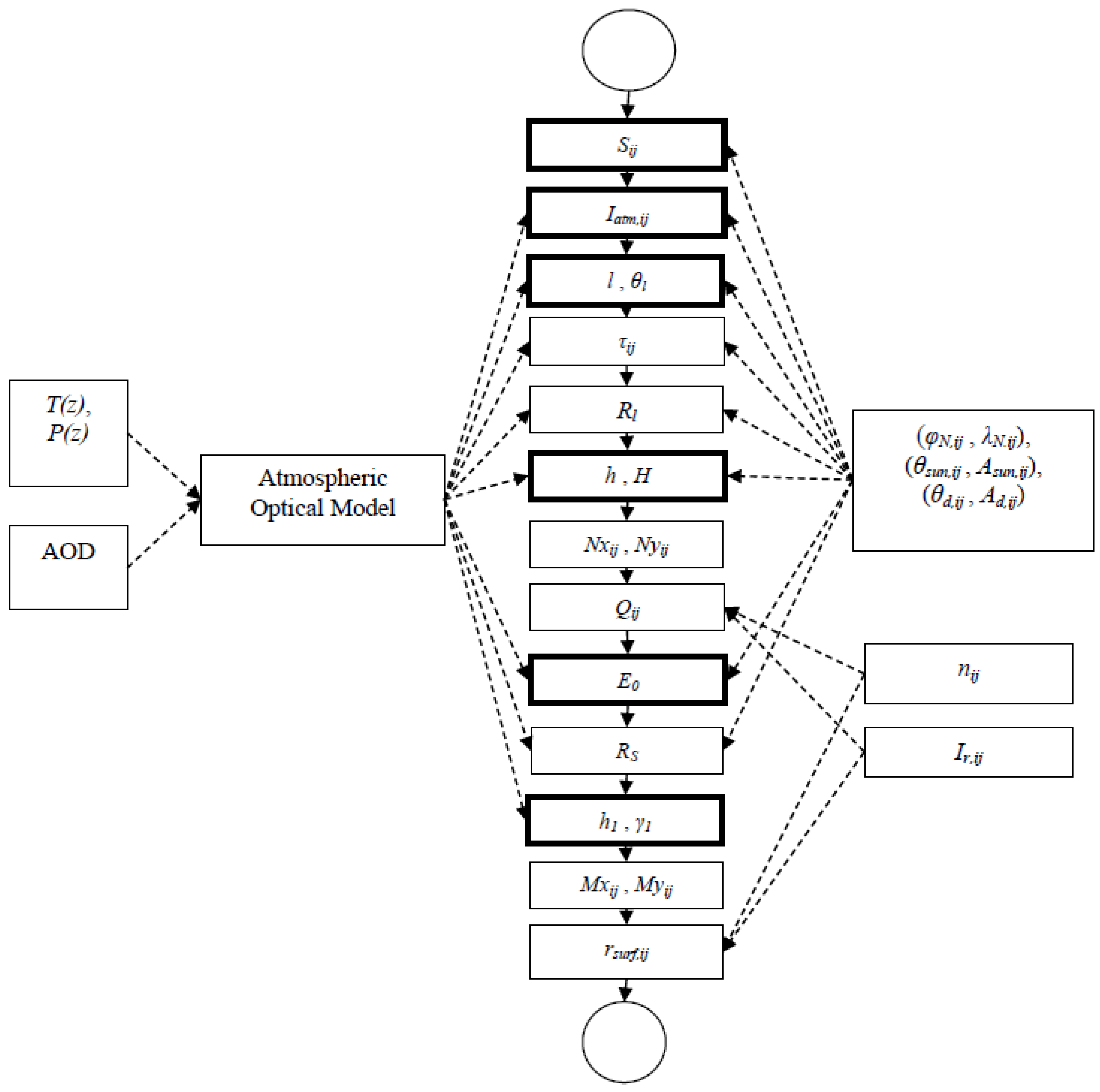
2.4. Block Diagram of the Algorithm

The block diagram of the proposed algorithm is shown in Figure 2. To estimate the ground surface reflectance, the following actions are performed:

• Formation of the block of input data. Input data are the following: radiance received in the MODIS band $I_{r,ij}$ (i is the pixel line number, j is the pixel column number); aerosol optical depth (AOD) of the atmosphere; vertical profiles of temperature $T\left(z\right)$ and pressure $P\left(z\right)$; cloud mask $n_{ij}$; information about the mutual positions of observed pixels, the sun, and the satellite (pixel coordinates (${\phi }_{N,ij},{\lambda }_{N,ij}$), direction to the sun (${\theta }_{sun,ij},A_{sun,ij}$), direction to the satellite (${\theta }_{d,ij},A_{d,ij}$)). These data can be borrowed from MODIS thematic products MOD021_L2, MOD03_L2, MOD07_L2, MOD35_L2, and MOD08_D3.
• Construction of the atmospheric model. Satellite measurements of AOD, $T\left(z\right)$, and $P\left(z\right)$ formed the basis for constructing the atmospheric model. Profiles of the aerosol extinction and scattering coefficients are set based on MODTRAN models [39] closest in the aerosol optical depth to MODIS data. Profiles of the molecular scattering coefficients are set based on the temperature and pressure profiles and the values of the molecular scattering coefficients from [40]. Profiles of the molecular absorption coefficients are constructed based on the vertical temperature and pressure profiles, the MODTRAN model of the gas composition of the atmosphere for mid-latitude summer, and absorption cross-sections of atmospheric gases from the HITRAN database [41]. The atmospheric models can be found in the Supplementary Materials [37]. The algorithm for construction of these models is described in Appendix A.
• Calculation of the areas $S_{ij}$. The image under consideration was divided into sections with respect to the closeness to the pixel centers. The algorithm for calculating the areas is described in the Supplementary Materials [37].
• Calculation of the radiance $I_{atm,ij}$ for the radiation non-interacting with the ground surface.
• Determination of the number l and angles of the boundaries ${\theta }_l$ of isoplanar zones (zones in which one PSF of the AE h can be used).
• Calculation of direct transmittance at the “observed pixel–receiver” path ${\tau }_{ij}$.
• Calculation of the AE radii for isoplanar zones $R_l$.
• Calculation of $h({\rho }_w,{\alpha }_w,{\mu }_l)$ for each isoplanar zone and its integral over the entire ground surface $H\left({\mu }_l\right)$.
• Estimation of the number of pixels in an image (in image lines $N{x}_{ij}$ and columns $N{y}_{ij}$) within the AE radius $R_l$ for each pixel.
• Solution of system of linear algebraic Equation (8) for luminosity of observed pixels $Q_{ij}$.
• Calculation of ground surface irradiance neglecting the reflected radiation $E_0$.
• Calculation of the radii $R_S$ of additional irradiance of the ground surface by surface pixels.
• Calculation of $h_1\left({\rho }_w\right)$ and its integral ${\gamma }_1$.
• Estimation of the number of pixels in an image (in image lines $M{x}_{ij}$ and columns $M{y}_{ij}$) within the radius of additional irradiance formation $R_S$ for each pixel.
• Solution of system of nonlinear Equation (9) for surface reflectance $r_{surf,ij}$.

To implement this algorithm, we have developed eight Monte Carlo programs for determining the following parameters: $S_{ij}$, $I_{atm,ij}$, $k_1\left({\rho }_w\right)$, $h({\theta }_l,{\rho }_w,{\alpha }_w)$, $H\left({\theta }_l\right)$, $E_0$, $h_1\left({\rho }_w\right)$, and ${\gamma }_1$ [27,38]. Let us touch briefly the approaches to simulation of these parameters. The radiance $I_{atm,ij}$ was simulated by the backward scheme with local estimates at collision point. The values of $k_1$, H, and h were calculated by the Monte Carlo algorithm based on direct trajectories from the same point on the surface as a Lambertian source with the trajectory turned at each collision point so that the collision point is on the line of sight. This algorithm is described in detail in [42]. The value of $E_0$ was calculated by the Monte Carlo program with backward trajectories from the ground surface and local estimates at collision points. The value of $h_1$ and ${\gamma }_1$ were determined through direct Monte Carlo simulation. Most of the developed programs (except for the programs for $k_1$, H, and h) were based on classical algorithms proposed in [43]. The Monte Carlo algorithms are considered in detail in Appendix B.

2.5. Algorithm Reliability

The reliability of results obtained with the developed Monte Carlo programs was checked in [27,38] through the comparison with the calculated data [44,45,46,47,48] and with analytical solutions in the single-scattering approximation. The performed comparisons allow us to state that, within the framework of the mentioned assumptions, the developed Monte Carlo programs provide reliable results.

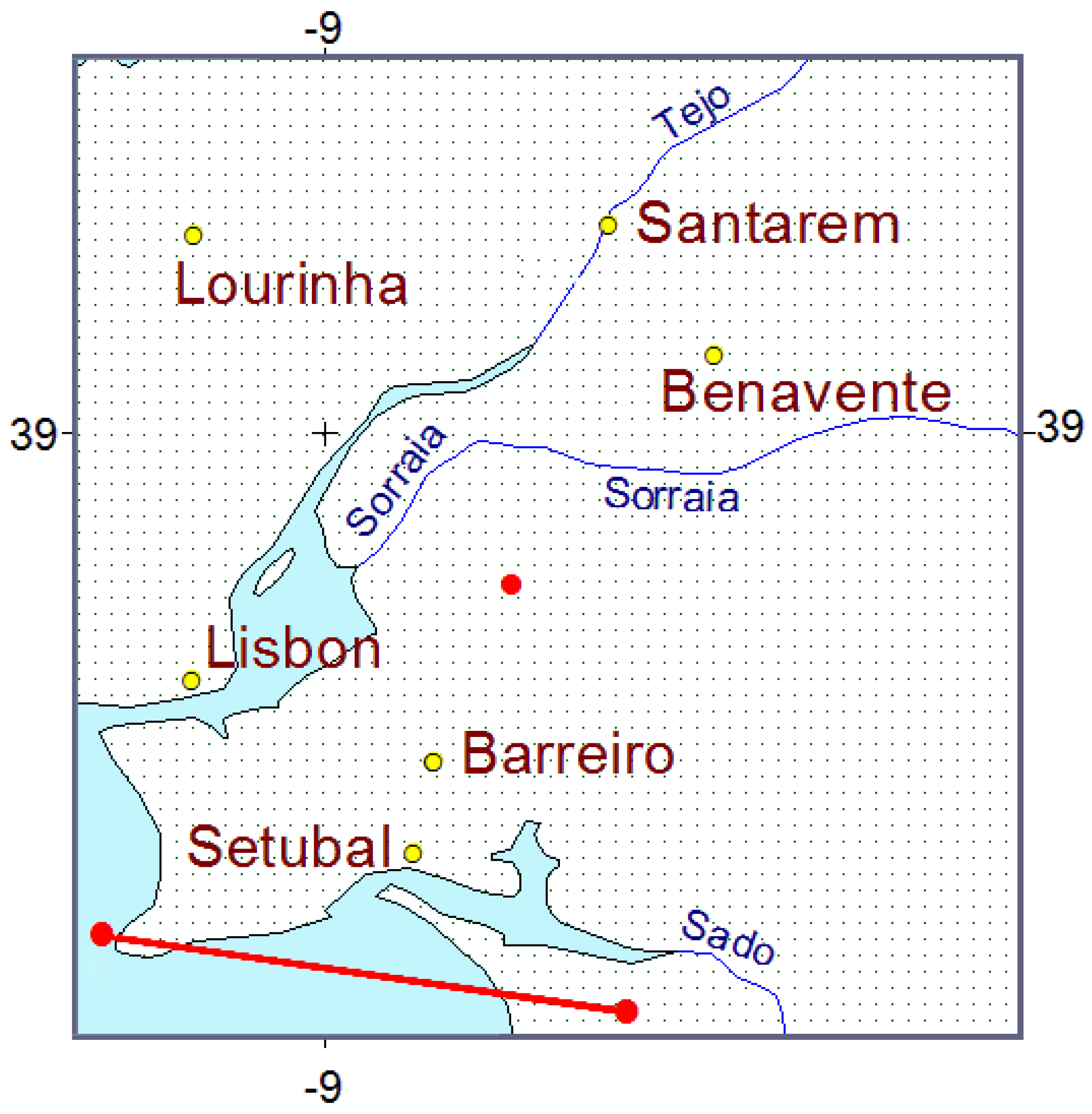
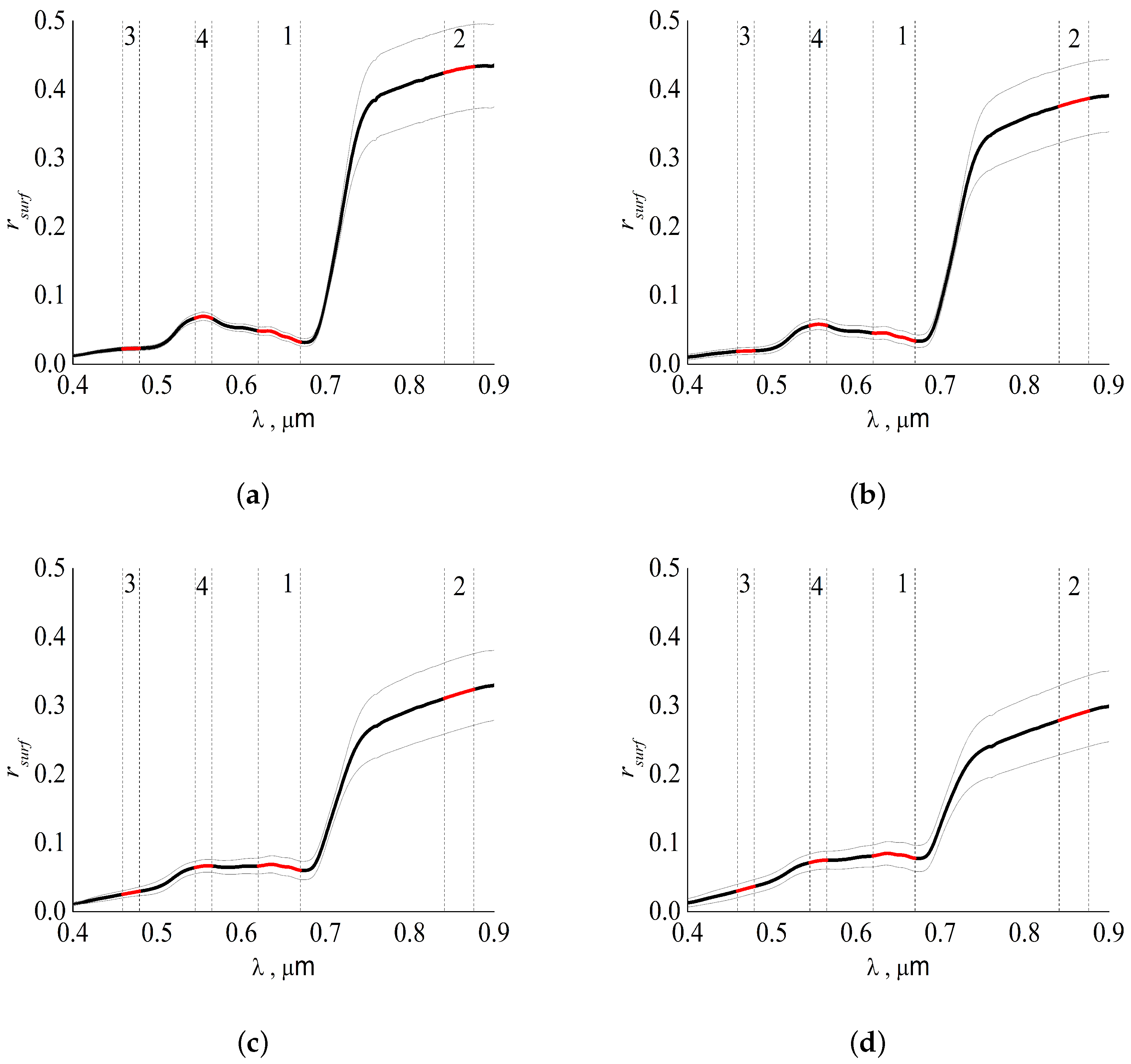
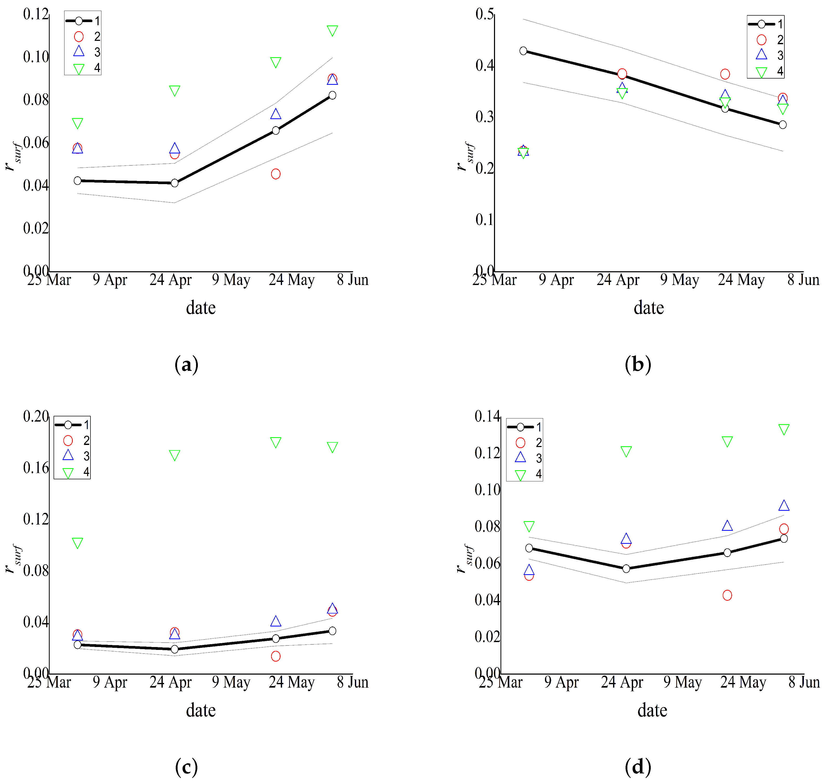
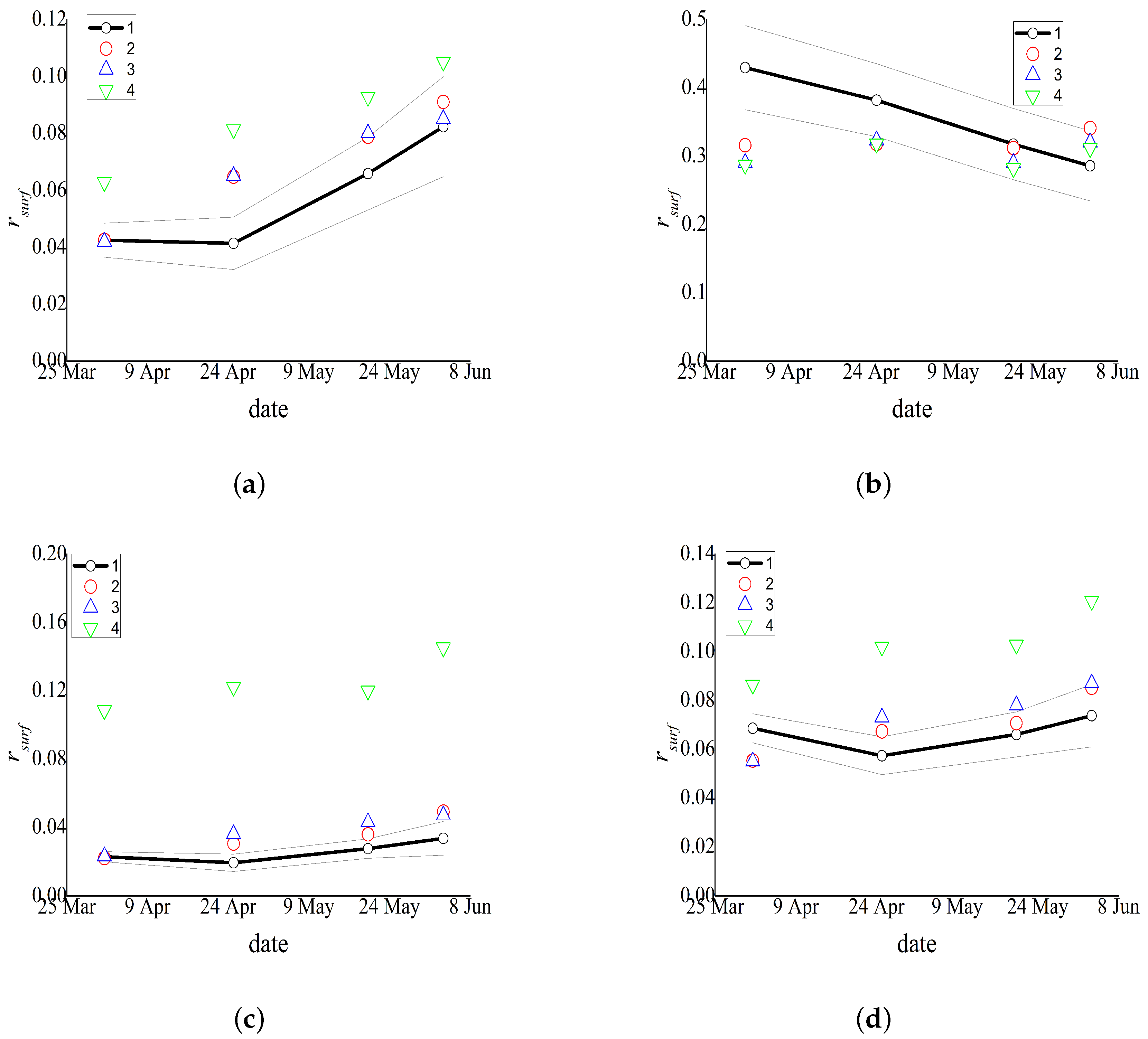
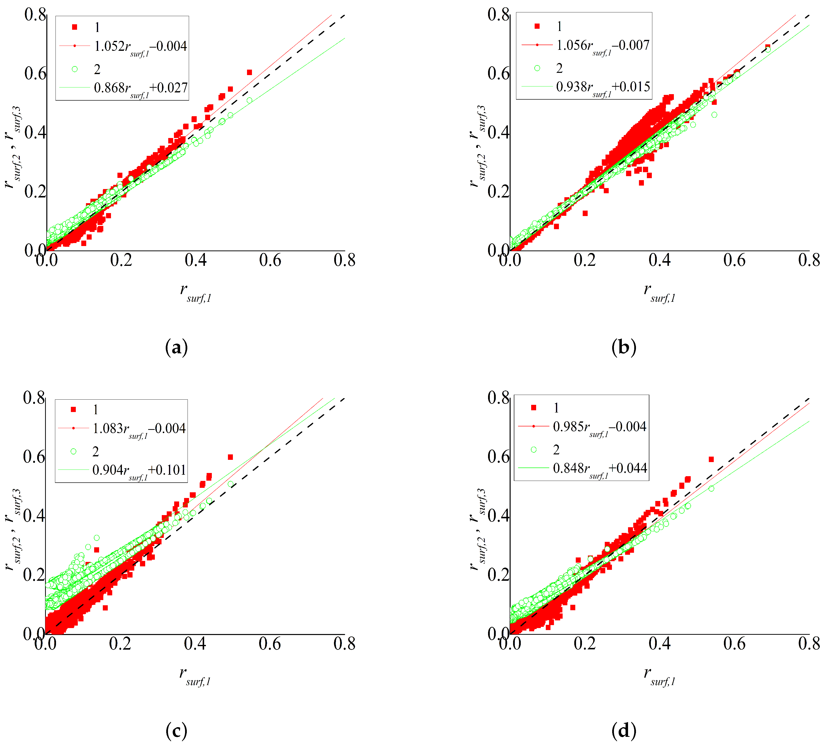
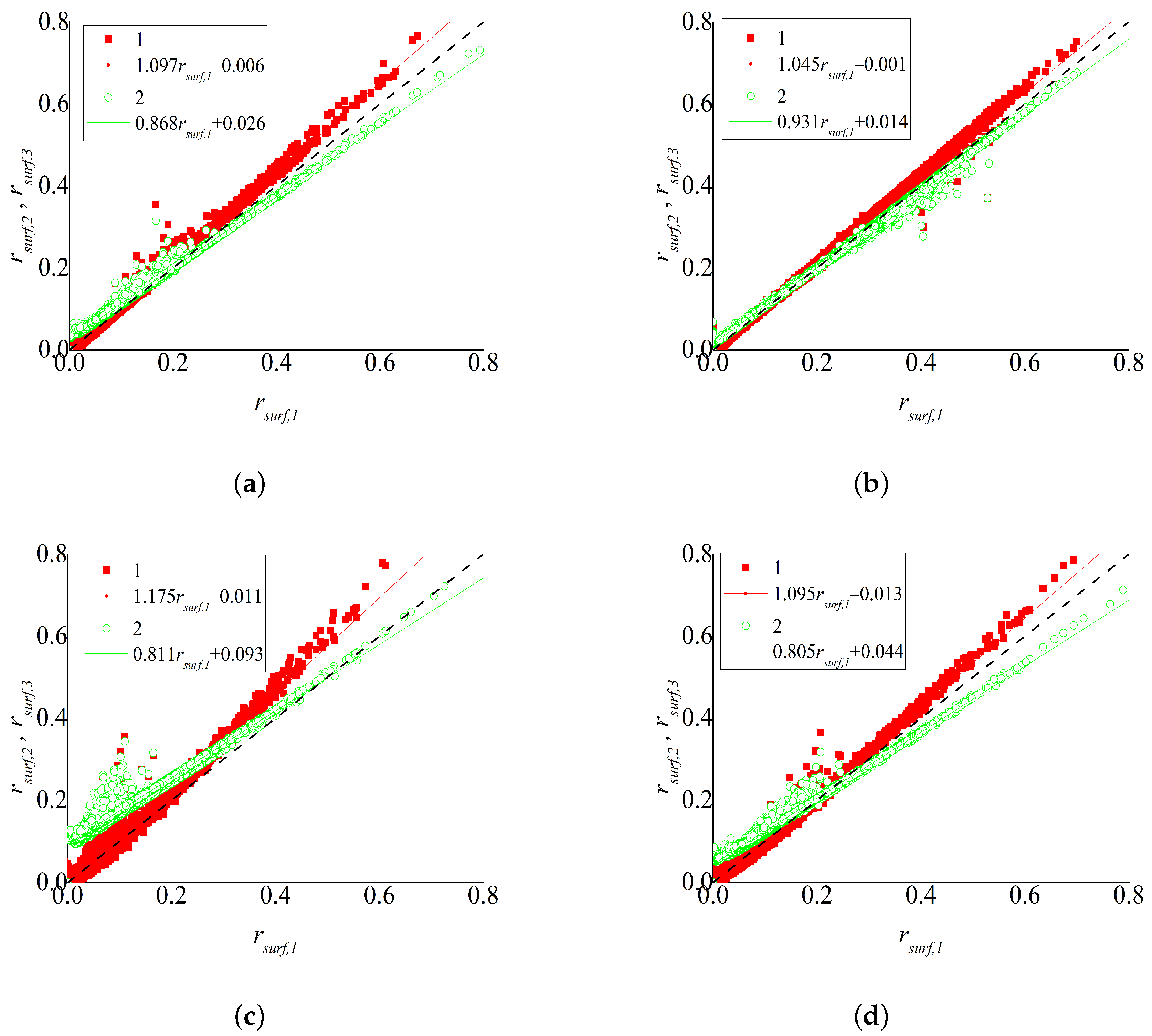
3. Algorithm Validation against Ground-Based Measurements

To assess the efficiency of the proposed algorithm, we have considered a test area with the coordinates 38.4–39.4${}^{°}$N, 8.25–9.25${}^{°}$W (Figure 3). For the site with the coordinates 38.829${}^{°}$N, 8.791${}^{°}$W (red dot in Figure 3) located at the center of this area, a series of ground-based measurements of surface reflectance was carried out in 2016 [28]. This is a Mediterranean grassland at Companhia das Lezirias, an estate of approximately 15,000 ha, located north-east of Lisbon, Portugal. Hyperspectral observations were performed using a FieldSpec3 spectroradiometer.

Measurements were taken at 24 closely spaced locations. The measured information can be an objective basis for validating the proposed algorithm. The test area is represented by grasslands. Thus, if the model results turn out to be close to the measured values of $r_{surf}$ for this area, then we can say that the algorithm is applicable for retrieving the reflectance of territories covered with vegetation in the growing season. The algorithm was validated in the following way. Measurements for 1 April, 25 April, 25 May, and 3 June of 2016 are available in [28]. They are hyperspectral measurements with a step of 0.001 $\mathsf{\mu }$m (Figure 4). These data were averaged over 24 sites and standard deviations were calculated. The data were averaged uniformly over wavelengths within the MODIS bands. The obtained averaged values and their standard deviation are given in

Table 2. Ground-based measurements for average wavelengths of MODIS bands and their standard deviations (SD).

	MODIS Band
Date	1		2		3		4
	${\mathit{r}}_{\mathit{surf}}$	SD	${\mathit{r}}_{\mathit{surf}}$	SD	${\mathit{r}}_{\mathit{surf}}$	SD	${\mathit{r}}_{\mathit{surf}}$	SD
1 April 2016	0.0425	0.0060	0.4295	0.0616	0.0228	0.0030	0.0686	0.0059
25 April 2016	0.0414	0.0092	0.3818	0.0533	0.0192	0.0051	0.0573	0.0077
20 May 2016	0.0659	0.0128	0.3175	0.0521	0.0275	0.0057	0.0661	0.0092
3 June 2016	0.0823	0.0176	0.2857	0.0512	0.0336	0.0098	0.0737	0.0127

.

For four MODIS bands of the TERRA and AQUA satellites (central wavelengths $\lambda$ = 0.645, 0.858, 0.469, and 0.555 $\mathsf{\mu }$m) for the same dates and the pixels closest to the test area, the data of Table 2 were compared with the reflectances $r_{surf}$ obtained by the proposed algorithm, the MOD09 algorithm, and the algorithm without atmospheric correction described by the following equation:

$$r_{surf,nocor,ij}=\frac{\pi I_{r,ij}}{S_{\lambda }{\mu }_{sun,ij}},$$

(19)

where $S_{\lambda }$ is the solar constant.

The comparison of the ground-based measurements with the results calculated by the three algorithms is performed in Figure 5 and Figure 6 and

Table 3. Discrepancy of the averaged ground-based measurements [28] and the results provided by the three algorithms for the TERRA data.

MODIS Band	Date	Proposed Algorithm	MOD09 Algorithm	Algorithm without Atmospheric Correction
1	1 April 2016	0.015	0.015	0.027
1	25 April 2016	0.014	0.016	0.044
1	20 May 2016	−0.020	0.007	0.032
1	3 June 2016	0.008	0.007	0.031
2	1 April 2016	−0.195	−0.197	−0.196
2	25 April 2016	0.003	−0.027	−0.032
2	20 May 2016	0.067	0.024	0.014
2	3 June 2016	0.052	0.044	0.033
3	1 April 2016	0.008	0.006	0.080
3	25 April 2016	0.013	0.011	0.152
3	20 May 2016	−0.014	0.012	0.154
3	3 June 2016	0.015	0.016	0.144
4	1 April 2016	−0.015	−0.013	0.012
4	25 April 2016	0.014	0.016	0.065
4	20 May 2016	−0.023	0.014	0.061
4	3 June 2016	0.005	0.017	0.060

and

Table 4. Discrepancy of the averaged ground-based measurements [28] and the results provided by the three algorithms for the AQUA data.

MODIS Band	Date	Proposed Algorithm	MOD09 Algorithm	Algorithm without Atmospheric Correction
1	1 April 2016	9.00 $\times {10}^{-5}$	−4.80 $\times {10}^{-4}$	0.020
1	25 April 2016	0.023	0.024	0.040
1	20 May 2016	0.013	0.014	0.027
1	3 June 2016	0.009	0.003	0.023
2	1 April 2016	−0.114	−0.140	−0.142
2	25 April 2016	−0.064	−0.059	−0.064
2	20 May 2016	−0.006	−0.028	−0.035
2	3 June 2016	0.055	0.034	0.026
3	1 April 2016	−0.001	2.20 $\times {10}^{-4}$	0.086
3	25 April 2016	0.011	0.017	0.103
3	20 May 2016	0.008	0.015	0.092
3	3 June 2016	0.016	0.013	0.112
4	1 April 2016	−0.013	−0.014	0.018
4	25 April 2016	0.010	0.016	0.045
4	20 May 2016	0.005	0.012	0.037
4	3 June 2016	0.011	0.013	0.047

. The obtained values of surface reflectances can be found in the Supplementary Materials [37]. The results obtained by the proposed algorithm and by the MOD09 algorithm demonstrate a good agreement with the ground-based data except for the results of 1 April 2016 for band 2 of the both satellites. For bands 1, 3, and 4, the discrepancy ranges from −0.023 to 0.023 for the proposed algorithm and from −0.014 to 0.024 for MOD09. For band 2, for all the considered days except for 1 April 2016, the discrepancy ranges from −0.064 to 0.067 for the proposed algorithm and from −0.059 to 0.044 for MOD09. The significant discrepancy for 1 April 2016 for band 2 is most likely reasoned by the difference between the used atmospheric models and the actual atmosphere. The comparison of the MOD09 results and the results of the proposed algorithm for the test site shows that they are in a good agreement for all the days for AQUA and for all the days except for 20 May 2016 for TERRA. The discrepancy for 20 May 2016 for the TERRA data is presumably due to differences in atmospheric models. For bands 1, 3, and 4, the results without atmospheric correction differ widely from the ground-based measurements, MOD09 results, and results provided by the proposed algorithm (the discrepancy from the ground-based measurements ranges from 0.012 to 0.154). As for band 2, for some days, the results without atmospheric correction are closer to the ground-based data than the MOD09 results and the results of our algorithm (for example, for the TERRA data for 20 May 2016). Thus, the proposed algorithm provides results no worse than the MOD09 algorithm for the test uniform area.

In addition, the results provided by the MOD09 algorithm, the proposed algorithm, and the algorithm without atmospheric correction were compared for the entire test area (38.4–39.4${}^{°}$N, 8.25–9.25${}^{°}$W), four analyzed days, and four MODIS bands. The results of comparison are shown in Figure 7 and Figure 8 and

Table 5. Pearson correlation r, average discrepancies $|\overline{\Delta r_{surf}}|$, and standard deviations (SD) of MOD09 results (1) from the results of the proposed algorithm (2) and algorithm without atmospheric correction (3) for the considered AQUA and TERRA data.

MODIS	No Correction			Proposed Algorithm
Band	r	SD	$\overline{\Delta {\mathit{r}}_{\mathit{surf}}}$	r	SD	$\overline{\Delta {\mathit{r}}_{\mathit{surf}}}$
AQUA
1	0.997	0.008	0.014	0.997	0.007	0.006
2	0.999	0.006	0.009	0.994	0.009	0.017
3	0.975	0.014	0.081	0.987	0.012	0.009
4	0.993	0.009	0.025	0.994	0.007	0.007
TERRA
1	0.986	0.010	0.010	0.984	0.006	0.004
2	0.999	0.005	0.003	0.985	0.015	0.007
3	0.734	0.052	0.060	0.948	0.009	0.005
4	0.948	0.018	0.020	0.963	0.008	0.006

. Figure 9, Figure 10 and Figure 11 exemplify the values of $r_{surf}$ obtained by the three algorithms for 1 April 2016. The analysis shows that the results of the MOD09 and proposed algorithms correlate with the coefficient greater than 0.94. The results without atmospheric correction are also strongly correlated with MOD09: the correlation coefficient is greater than 0.73 for MODIS band 3 and 0.94 for all the other bands. The average discrepancy between the results of the proposed algorithm and MOD09 does not exceed 0.009 for bands 1, 3, and 4 and 0.017 for band 2. Based on the high correlation of the results provided by the algorithms, linear regressions were constructed (shown in Figure 7 and Figure 8). The analysis of the regressions shows that, for nearly all the considered situations (except for TERRA band 4) for surfaces with the reflectance close to zero, the MOD09 values are, on average, higher than those of the proposed algorithm, but for the surface with high reflectance, the values given by the proposed algorithm are higher. This situation is likely due to the fact that the proposed algorithm better takes into account the effect that low-reflective surfaces seem more reflective due to the adjacency effect from highly reflective surfaces and vice versa. The analysis of the regression between MOD09 and the algorithm without correction shows that, for low-reflective surface, the algorithm without atmospheric correction gives values higher than those of MOD09. This is primarily due to the fact that the algorithm without atmospheric correction ignores the influence of solar radiation non-interacting with the ground surface.

In the southwestern part of the test area, where some territories are covered with water, the MOD09 algorithm often gives negative values of reflectance for the considered days. For example, for 1 April 2016 for the TERRA data, it yields negative reflectance for 4.8% of cloudless pixels in band 1, 5.9% in band 2, 3.8% in band 3, and 2.7% in band 4. At the same time, the proposed algorithm gives significantly fewer negative values for water areas (for example, for the same day for the TERRA data, 2.1% negative reflectance values for band 1 and 0% for the other bands). As an example, Figure 12 shows the values of $r_{surf}$ for one of the image lines from the pixel with coordinates 38.351${}^{°}$N, 8.660${}^{°}$W to the pixel with coordinates 38.438${}^{°}$N, 9.247${}^{°}$W (red line in Figure 3) as provided by the three analyzed algorithms. It can be seen that the MOD09 algorithm gives zero and negative reflectances for the most pixels in fragments with low reflectance. The proposed algorithm gives much fewer negative results (Figure 12a) or only positive results (Figure 12b–d). For the situation under consideration, the MOD09 atmospheric model and the one we used differed. However, test comparisons for a uniform area (Table 3 and Table 4) allow us to state that the main reason for the differences is how the algorithm we propose takes into account the adjacency effect and additional illumination by reflected radiation. Thus, the advantage of the proposed algorithm in comparison with MOD09 manifests itself in surface areas with a significant change in reflectance.

4. Conclusions

Following our analysis, the following most important results have been obtained:

(1) Comparison of the results provided by the proposed algorithm and the MOD09 algorithm based on TERRA and AQUA data with ground-based measurements for the area with coordinates 38.829${}^{°}$N, 8.791${}^{°}$W demonstrates a good agreement.

(2) For bands 1, 3, and 4, the discrepancy between the calculated results and the ground-based measurements [28] ranges from −0.023 to 0.023 for the proposed algorithm and from −0.014 to 0.024 for MOD09. For band 2, for all the analyzed days except for 1 April 2016, the discrepancy ranges from −0.064 to 0.067 for the proposed algorithm and from −0.059 to 0.044 for MOD09.

(3) The comparison of the results provided by the MOD09 algorithm and the proposed algorithm for the area with coordinates 38.4–39.4${}^{°}$N, 8.25–9.25${}^{°}$W for all the four analyzed days and four MODIS bands shows that they correlate with the coefficient higher than 0.94. The average discrepancy between the results for the both algorithms does not exceed 0.009 for bands 1, 3, and 4 and 0.017 for band 2.

(4) An analysis of the regressions between the results of MOD09 and the proposed algorithm shows that the values of MOD09 are, on average, higher than those of the proposed algorithm for surfaces with reflectance close to zero, but the values obtained by the proposed algorithm are higher for surfaces with high reflectance.

(5) For fragments with low reflectance (water surfaces), MOD09 algorithm often gives zero or negative reflectance values for the considered pixels. At the same time, the proposed algorithm gives either much fewer negative results (Figure 12a) or only positive values (Figure 12b–d).

The use of the criterion of separation of isoplanar zones in the proposed algorithm and similar algorithms allows one to set the error level and to calculate the needed number of PSFs for a given image, a receiver band, and observation conditions by Equation (10). Criteria (13) and (15) for estimating the radii of the adjacency effect and formation of additional irradiance of the ground surface allow obtaining the upper estimate of the size of zones, outside of which these effects are small. The proposed criteria are suitable for use in all alternative algorithms that take into account the adjacency effect and the influence of the inhomogeneity of surface reflection in formation of surface illumination. Interpolation Equations (16)–(18) for the radiation non-interacting with the surface can also be used in similar algorithms.

The comparison with the ground-based measurements and MOD09 data for TERRA and AQUA satellite data shows that, for the uniform surface area, the proposed algorithm gives results no worse than MOD09: in some days, our results are closer to the average ground-based measurements, while, in others, the MOD09 results are closer. The test area was chosen because the data of ground-based measurements are available for it [28]. The proposed algorithm can be used for other surface areas as well. In the future, we plan to expand significantly the set of ground-based data, for which the algorithm was validated, to such data as RadCalNet [49].

The employed atmospheric model uses data on the aerosol optical depth and temperature and pressure profiles as input data. Obtaining these data is a separate problem. The algorithm allows using other atmospheric models. Its operation requires profiles of the aerosol and molecular extinction and scattering coefficients, as well as aerosol scattering phase function, which can be obtained by various methods.

The adjacency effect is even more important for medium and high spatial resolution images than for low resolution images. The MODIS data were chosen for the comparison due to the high capabilities of the MOD09 algorithm, which allows better testing of the proposed algorithm. The proposed method can be readily adapted to use with other satellite devices having bands in the visible and NIR ranges. In the future, the applicability of the proposed algorithm will be extended to satellites of medium and high spatial resolution, such as Landsat and Russian Kanopus-V and Meteor-M satellites. Currently, the method cannot be used in batch mode yet. In the current version, the processing of a 5-minute MODIS image takes about 2 h of PC time (16 × AMD Ryzen 7 1800X Eight-Core Processor). In the nearest future, it is planned to adapt the software package for cluster operation in batch mode.

Factors such as the non-Lambertian character of reflection and the surface topography remain beyond the scope of this study. In the further studies, we plan to take into account the non-Lambertian reflection in the same way as in [29]. The surface topography is an important factor only for surfaces with significant height difference. It can be included in consideration by adding factors taking into account that a part of the solid angle can be overlapped by surfaces of adjacent fragments in Equations (8) and (9).

In general, the proposed algorithm contributes significantly to the solution of some problems arising when considering the adjacency effect and additional surface illumination, and it can be used for a wide range of atmospheric correction problems.

References

1. Otterman, J.; Fraser, R.S. Adjacency effects on imaging by surface reflection and atmospheric scattering: Cross radiance to zenith. Appl. Opt. 1979, 18, 2852–2860. [Google Scholar] [CrossRef]
2. Vanhellemont, Q.; Ruddick, K. Turbid wakes associated with offshore wind turbines observed with Landsat 8. Remote Sens. Environ. 2014, 145, 105–115. [Google Scholar] [CrossRef]
3. Cox, C.; Munk, W. Measurement of the Roughness of the Sea Surface from Photographs of the Sun’s Glitter. J. Opt. Soc. Am. 1954, 44, 838–850. [Google Scholar] [CrossRef]
4. Warren, M.A.; Simis, S.G.H.; Martinez-Vicente, V.; Poser, K.; Bresciani, M.; Alikas, K.; Spyrakos, E.; Giardino, C.; Ansper, A. Assessment of atmospheric correction algorithms for the Sentinel-2A MultiSpectral Imager over coastal and inland waters. Remote Sens. Environ. 2019, 225, 267–289. [Google Scholar] [CrossRef]
5. Wang, J.; Wang, Y.; Lee, Z.; Wang, D.; Chen, S.; Lai, W. A revision of NASA SeaDAS atmospheric correction algorithm over turbid waters with artificial Neural Networks estimated remote-sensing reflectance in the near-infrared. ISPRS J. Photogramm. Remote Sens. 2022, 194, 235–249. [Google Scholar] [CrossRef]
6. Tanre, D.; Herman, M.; Deschamps, P.Y.; de Leffe, A. Atmospheric modeling for space measurements of ground reflectances, including bidirectional properties. Appl. Opt. 1979, 18, 3587–3594. [Google Scholar] [CrossRef] [PubMed]
7. Putsay, M. A simple atmospheric correction method for the short wave satellite images. International J. Remote Sens. 1992, 13, 1549–1558. [Google Scholar] [CrossRef]
8. Berk, A.; Adler-Golden, S.M.; Ratkowski, A.J.; Felde, G.W.; Anderson, G.P.; Hoke, M.L.; Cooley, T.; Chetwynd, J.H.; Gardne, J.A.; Matthew, M.W.; et al. Exploiting MODTRAN radiation transport for atmospheric correction: The FLAASH algorithm. In Proceedings of the Fifth International Conference on Information Fusion. FUSION 2002 (IEEE Cat.No.02EX5997), Annapolis, MD, USA, 8–11 July 2002; pp. 798–803. [Google Scholar]
9. Vermote, E.F.; Vermeulen, A. Atmospheric Correction Algorithm: Spectral Reflectances (MOD09). Algorithm Theoretical Background Document, Version 4.0. 1999. Available online: http://modis.gsfc.nasa.gov/data/atbd/atbd_mod08.pdf (accessed on 30 January 2023).
10. Lyapustin, A.; Wang, Y.; Korkin, S.; Huang, D. MODIS Collection 6 MAIAC algorithm. Atmos. Meas. Tech. 2018, 11, 5741–5765. [Google Scholar] [CrossRef]
11. Reinersman, P.N.; Carder, K.L. Monte Carlo simulation of the atmospheric point-spread function with an application to correction for the adjacency effect. Appl. Opt. 1995, 34, 4453–4471. [Google Scholar] [CrossRef]
12. Katkovsky, L.V.; Martinov, A.O.; Siliuk, V.A.; Ivanov, D.A.; Kokhanovsky, A.A. Fast Atmospheric Correction Method for Hyperspectral Data. Remote Sens. 2018, 10, 1698. [Google Scholar] [CrossRef]
13. Shi, H.; Xiao, Z. The 4SAILT Model: An Improved 4SAIL Canopy Radiative Transfer Model for Sloping Terrain. IEEE Trans. Geosci. Remote Sens. 2021, 59, 5515–5525. [Google Scholar] [CrossRef]
14. Tanre, D.; Holben, B.N.; Kaufman, Y.J. Atmospheric correction algorithm for NOAA-AVHRR products: Theory and application. IEEE Trans. Geosci. Remote Sens. 1992, 30, 231–248. [Google Scholar] [CrossRef]
15. Zimovaya, A.V.; Tarasenkov, M.V.; Belov, V.V. Radiation Polarization Effect on the Retrieval of the Earth’s Surface Reflection Coefficient from Satellite Data in the Visible Wavelength Range. Atmos. Ocean. Opt. 2018, 31, 131–136. [Google Scholar] [CrossRef]
16. Kotchenova, S.Y.; Vermote, E.F.; Matarrese, R.; Klemm, F.J. Validation of a vector version of the 6S radiative transfer code for atmospheric correction of satellite data. Part I: Path radiance. Appl. Opt. 2006, 45, 6762–6774. [Google Scholar] [CrossRef]
17. Cahalan, R.F.; Oreopoulos, L.; Wen, G.; Marshak, A.; Tsay, S.-C.; DeFelice, T. Cloud characterization and clear-sky correction from Landsat-7. Remote Sens. Environ. 2002, 78, 83–98. [Google Scholar] [CrossRef]
18. Wen, G.; Marshak, A.; Cahalan, R.F.; Remer, L.A.; Kleidman, R.G. 3-D aerosol-cloud radiative interaction observed in collocated MODIS and ASTER images of cumulus cloud fields. J. Geophys. Res. 2007, 112, D13204. [Google Scholar] [CrossRef]
19. Varnai, T.; Marshak, A. MODIS observations of enhanced clear sky reflectance near clouds. Geophys. Res. Lett. 2009, 36, L06807. [Google Scholar] [CrossRef]
20. Marshak, A.; Evans, K.F.; Varnai, T.; Wen, G. Extending 3D near-cloud corrections from shorter to longer wavelengths. J. Quant. Spectrosc. Radiat. Transf. 2014, 147, 79–85. [Google Scholar] [CrossRef]
21. Tarasenkov, M.V.; Engel, M.V.; Zonov, M.N.; Belov, V.V. Assessing the Cloud Adjacency Effect on Retrieval of the Ground Surface Reflectance from MODIS Satellite Data for the Baikal Region. Atmosphere 2022, 13, 2054. [Google Scholar] [CrossRef]
22. Richter, R.; Schläpfer, D. ATCOR-2/3 User Guide; ReSe Applications Schläpfer: Wil, Switzerland, 2012; p. 203. [Google Scholar]
23. Craig J., M. Performance assessment of ACORN atmospheric correction algorithm. In Proceedings of the SPIE 4725, Algorithms and Technologies for Multispectral, Hyperspectral, and Ultraspectral Imagery VIII, AeroSense 2002, Orlando, FL, USA, 2 August 2002. [Google Scholar] [CrossRef]
24. Gao, B.-C.; Heidebrecht, K.B.; Goetz, A.F.H. Atmosphere Removal Program (ATREM) Version 3.1 Users Guide; Center for the Study of Earth from Space (CSES), Cooperative Institute for Research in Environmental Sciences (CIRES), University of Colorado: Boulder, CO, USA, 1996. [Google Scholar]
25. Adler-Golden, S.M.; Matthew, M.W.; Bernstein, L.S.; Levine, R.Y.; Berk, A.; Richtsmeier, S.C.; Acharya, P.K.; Anderson, G.P.; Felde, J.W.; Gardner, J.A.; et al. Atmospheric correction for shortwave spectral imagery based on MODTRAN4. Proc. SPIE Imaging Spectrom. V 1999, 3753. [Google Scholar] [CrossRef]
26. Qu, Z.; Kindel, B.C.; Goetz, A.F.H. The High Accuracy Atmospheric Correction for Hyperspectral Data (HATCH) model. IEEE Trans. Geosci. Remote Sens. 2003, 41, 1223–1231. [Google Scholar]
27. Tarasenkov, M.V.; Zimovaya, A.V.; Belov, V.V.; Engel, M.V. Retrieval of Reflection Coefficients of the Earth’s Surface from MODIS Satellite Measurements Considering Radiation Polarization. Atmos. Ocean. Opt. 2020, 33, 179–187. [Google Scholar] [CrossRef]
28. Cerasoli, S.; Campagnolo, M.; Faria, J.; Nogueira, C.; Caldeira, M.D.C. On estimating the gross primary productivity of Mediterranean grasslands under different fertilization regimes using vegetation indices and hyperspectral reflectance. Biogeosciences 2018, 15, 5455–5471. [Google Scholar] [CrossRef]
29. Vermote, E.; Justice, C.O.; Breon, F.-M. Towards a Generalized Approach for Correction of the BRDF Effect in MODIS Directional Reflectances. IEEE Trans. Geosci. Remote Sens. 2009, 47, 898–908. [Google Scholar] [CrossRef]
30. Roujean, J.-L.; Leroy, M.; Deschamps, P.-Y. A bidirectional reflectance model of the Earth’s surface for the correction of remote sensing data. J. Geophys. Res. 1992, 97, 20455–20468. [Google Scholar] [CrossRef]
31. Rahman, H.; Pinty, B.; Verstraete, M.M. Coupled surface-atmosphere reflectance (CSAR) model: 2. Semiempirical surface model usable with NOAA advanced very high resolution radiometer data. J. Geophys. Res. 1993, 98, 20791–20801. [Google Scholar] [CrossRef]
32. Verhoef, W.; Bach, H. Remote sensing data assimilation using coupled radiative transfer models. Phys. Chem. Earth Parts A/B/C 2003, 28, 3–13. [Google Scholar] [CrossRef]
33. Maignan, F.; Breon, F.-M.; Lacaze, R. Bidirectional reflectance of Earth targets: Evaluation of analytical models using a large set of spaceborne measurements with emphasis on the Hot Spot. Remote Sens. Environ. 2004, 90, 210–220. [Google Scholar] [CrossRef]
34. Mousivand, A.; Verhoef, W.; Menenti, M.; Gorte, B. Modeling Top of Atmosphere Radiance over Heterogeneous Non-Lambertian Rugged Terrain. Remote Sens. 2015, 7, 8019–8044. [Google Scholar] [CrossRef]
35. Jia, W.; Pang, Y.; Tortini, R.; Schlapfer, D.; Li, Z.; Roujean, J.-L. A Kernel-Driven BRDF Approach to Correct Airborne Hyperspectral Imagery over Forested Areas with Rugged Topography. Remote Sens. 2020, 12, 33. [Google Scholar] [CrossRef]
36. NOAA National Centers for Environmental Information. 2022: ETOPO 2022 15 Arc-Second Global Relief Model. NOAA National Centers for Environmental Information. Available online: https://data.noaa.gov/metaview/page?xml=NOAA/NESDIS/NGDC/MGG/DEM//iso/xml/etopo_2022.xml&view=getDataView&header=none (accessed on 30 January 2023).
37. Supplementary Material. Available online: https://github.com/MarinaEngel/Atmosphere_2023 (accessed on 31 January 2023).
38. Tarasenkov, M.V.; Belov, V.V.; Engel, M.V. Algorithm for reconstruction of the Earth surface reflectance from Modis satellite measurements in a turbid atmosphere. In Proceedings of the SPIE 10833, 24th International Symposium on Atmospheric and Ocean Optics: Atmospheric Physics, Tomsk, Russia, 2–5 July 2018; Volume 10833, pp. 1–16. [Google Scholar]
39. Kneizys, F.X.; Robertson, D.C.; Abreu, L.W.; Acharya, P.; Anderson, G.P.; Rothman, L.S.; Chetwynd, J.H.; Selby, J.E.A.; Shettle, E.P.; Gallery, W.O.; et al. The MODTRAN 2/3 Report and LOWTRAN 7 Model; U.S. Air Force Geophysics Laboratory: Hanscom, MA, USA, 1996. [Google Scholar]
40. Bucholtz, A. Rayleigh-scattering calculations for the terrestrial atmosphere. Appl. Opt. 1995, 34, 2765–2773. [Google Scholar] [CrossRef] [PubMed]
41. HITRAN Database. Available online: https://hitran.org/ (accessed on 30 January 2023).
42. Belov, V.V.; Tarasenkov, M.V. Statistical Modeling of the Point Spread Function in the Spherical Atmosphere and a Criterion for Detecting Image Isoplanarity Zones. Atmos. Ocean. Opt. 2010, 23, 441–447. [Google Scholar] [CrossRef]
43. Marchuk, G.I.; Mikhailov, G.A.; Nazaraliev, M.A.; Darbinjan, R.A.; Kargin, B.A.; Elepov, B.S. The Monte Carlo Methods in Atmospheric Optics; Springer: Berlin/Heidelberg, Germany, 1980. [Google Scholar]
44. Coulson, K.; Dave, J.; Sekera, Z. Tables Related to Radiation Emerging from a Planetary Atmosphere with Rayleigh Scattering; University of California Press: Berkeley, CA, USA, 1960; pp. 56–58. [Google Scholar]
45. Mekler, Y.; Kaufman, Y.J. Contrast reduction by the atmosphere and retrieval of nonuniform surface reflectance. Appl. Opt. 1982, 21, 310–316. [Google Scholar] [CrossRef] [PubMed]
46. Lenoble, J. Radiative Transfer in Scattering and Absorbing Atmospheres: Standard Computational Procedures; Deepak, A., Ed.; American Meteorological Society: Boston, MA, USA, 1985; p. 314. [Google Scholar]
47. Lenoble, J. Modeling of the Influence of Snow Reflectance on Ultraviolet Irradiance for Cloudless Sky. Appl. Opt. 1998, 37, 2441–2447. [Google Scholar] [CrossRef]
48. International Working Group on Polarized Radiative Transfer (IPRT). Available online: https://www.meteo.physik.uni-muenchen.de/~iprt/doku.php?id=start (accessed on 30 January 2023).
49. Radiometric Calibration Network Portal. Available online: https://www.radcalnet.org/ (accessed on 30 January 2023).
Figure 1. Optical fluxes forming the received radiation (according to [6]): (a) radiation that does not interact with the ground surface; (b) direct solar radiation that interacts with the surface fragment under study; (c) diffuse solar radiation that interacts with the surface fragment under study; (d) adjacency effect (AE) due to single reflected radiation; (e) adjacency effect due to multiple reflected radiation.
Remotesensing 15 02655 g001
Figure 2. Block diagram of the algorithm for retrieval of surface reflectance. Units employing the Monte Carlo method are shown in black.
Remotesensing 15 02655 g002
Figure 3. Test surface area with the coordinates 38.4–39.4 ° N, 8.25–9.25 ° W. The red dot is for the test site with the coordinates 38.829 ° N, 8.791 ° W, for which the results of ground-based measurements are reported in [28]. A red line is drawn from the pixel with coordinates 38.351 ° N, 8.660 ° W to the pixel with coordinates 38.438 ° N, 9.247 ° W.
Remotesensing 15 02655 g003
Figure 4. Ground-based measurements of reflectances of the surface area with coordinates 38.829 ° N, 8.791 ° W [28]: (a) 1 April 2016; (b) 25 April 2016; (c) 20 May 2016; (d) 3 June 2016. Numbers 1–4 are the numbers of the MODIS bands; thick lines are the average reflectances; thin lines are their standard deviations.
Remotesensing 15 02655 g004
Figure 5. Comparison of averaged ground-based measurements [28] and the results provided by the three algorithms for the TERRA data: (1) averaged ground-based measurements and their standard deviations (gray), (2) proposed algorithm, (3) MOD09, (4) without atmospheric correction; MODIS band 1 ( λ = 0.62–0.67 μ m) (a), 2 ( λ = 0.841–0.876 μ m) (b), 3 ( λ = 0.459–0.479 μ m) (c), and 4 ( λ = 0.545–0.565 μ m) (d).
Remotesensing 15 02655 g005
Figure 6. Comparison of averaged ground-based measurements [28] and the results provided by the three algorithms for the AQUA data: (1) averaged ground-based measurements and their standard deviations (gray), (2) proposed algorithm, (3) MOD09, (4) without atmospheric correction; MODIS band 1 ( λ = 0.62–0.67 μ m) (a), 2 ( λ = 0.841–0.876 μ m) (b), 3 ( λ = 0.459–0.479 μ m) (c), and 4 ( λ = 0.545–0.565 μ m) (d).
Remotesensing 15 02655 g006
Figure 7. Comparison of reflectances provided by MOD09 (plotted along the Ox axis), the proposed algorithm (symbols 1), and the algorithm without atmospheric correction (symbols 2) (plotted along the Oy axis) for TERRA; MODIS band 1 ( λ = 0.62–0.67 μ m) (a), 2 ( λ = 0.841–0.876 μ m) (b), 3 ( λ = 0.459–0.479 μ m) (c), and 4 ( λ = 0.545–0.565 μ m) (d).
Remotesensing 15 02655 g007
Figure 8. Comparison of reflectances provided by MOD09 (plotted along the Ox axis), the proposed algorithm (symbols 1), and the algorithm without atmospheric correction (symbols 2) (plotted along the Oy axis) for AQUA; MODIS band 1 ( λ = 0.62–0.67 μ m) (a), 2 ( λ = 0.841–0.876 μ m) (b), 3 ( λ = 0.459–0.479 μ m) (c), and 4 ( λ = 0.545–0.565 μ m) (d).
Remotesensing 15 02655 g008
Figure 9. Example of reflectances calculated by the proposed algorithm for four MODIS bands (TERRA, 1 April 2016). The values below 0 correspond to negative reflectance. MODIS band 1 ( λ = 0.62–0.67 μ m) (a), 2 ( λ = 0.841–0.876 μ m) (b), 3 ( λ = 0.459–0.479 μ m) (c), and 4 ( λ = 0.545–0.565 μ m) (d).
Remotesensing 15 02655 g009
Figure 10. Example of reflectances calculated by the MOD09 algorithm for four MODIS bands (TERRA, 1 April 2016). The values below 0 correspond to negative reflectance. MODIS band 1 ( λ = 0.62–0.67 μ m) (a), 2 ( λ = 0.841–0.876 μ m) (b), 3 ( λ = 0.459–0.479 μ m) (c), and 4 ( λ = 0.545–0.565 μ m) (d).
Remotesensing 15 02655 g010
Figure 11. Example of reflectances calculated by the algorithm without atmospheric correction for four MODIS bands (TERRA, 1 April 2016). MODIS band 1 ( λ = 0.62–0.67 μ m) (a), 2 ( λ = 0.841–0.876 μ m) (b), 3 ( λ = 0.459–0.479 μ m) (c), and 4 ( λ = 0.545–0.565 μ m) (d).
Remotesensing 15 02655 g011
Figure 12. Values of reflectance obtained by the three algorithms for line 879 of the TERRA image of the test area for 1 April 2016 from the pixel with coordinates 38.351 ° N, 8.660 ° W to the pixel with coordinates 38.438 ° N, 9.247 ° W. Negative values of r s u r f are omitted. The distance to the pixel with coordinates 38.351 ° N, 8.660 ° W is plotted along the Ox axis: (1) proposed algorithm; (2) MOD09 algorithm; (3) without atmospheric correction; MODIS band 1 ( λ = 0.62–0.67 μ m) (a), 2 ( λ = 0.841–0.876 μ m) (b), 3 ( λ = 0.459–0.479 μ m) (c), and 4 ( λ = 0.545–0.565 μ m) (d).
Remotesensing 15 02655 g012