A Block-Scale FFT Filter Based on Spatial Autocorrelation Features of Speckle Noise in SAR Image

Abstract

In order to reduce the impact of noise on the accuracy of inversion products based on SAR images, many filtering algorithms have been developed for noise reduction of SAR images. This paper proposes a filtering method based on the spatial autocorrelation feature of the block fast Fourier transform (BFFT). The method statistically analyses the autocorrelation length of speckle noise on Sentinel-1B images for different features and then constructs a relationship between autocorrelation length and noise period. After that, the size of the optimal FFT filtering window radius was determined based on the relationship between the noise period and the components in the image frequency domain. Finally, we filtered the SAR image within the parcels. We compared BFFT with six commonly used filtering methods. The results show that: (1) The noise periods of the soybean, corn, paddy, and water objects on the SAR image have little difference, with noise periods of 3.36, 3.17, 3.13, and 3.14 pixels on the VV polarization and 3.49, 3.17, 2.94, and 2.42 pixels on the VH polarization; (2) after the BFFT filtering in the land parcel area, the mean value of the backscattering coefficient (BC) kept constant, whilst at the same time, the standard deviation (STD) was reduced to half of that before the filtering and (3) the BFFT and NLM filtering methods have a better effect on noise reduction inside the block. The BFFT filtering method retains the variation trend between different regions within the block and preserves the block boundary’s clarity. This study provides a new idea for refined image processing.

1. Introduction

Synthetic Aperture Radar (SAR) is an active imaging system that emits microwaves that can penetrate clouds and fog, and the imaging conditions are not affected by time or weather. SAR is one of the significant data sources for obtaining surface information. Speckle appearing in SAR images is generated by coherent interference of radar echoes from target scatters [1]. During the acquisition of the SAR images, the echo signal received by each resolution unit is the result of the reflected waves of a large number of randomly distributed scattered beams [2]. Because the amplitude and phase of the echo signal of each scattering unit are different, there are fluctuations between other pixels in the actual obtained SAR intensity image, commonly known as coherent speckle noise [3,4].

Many filtering algorithms have been proposed to reduce speckle noise to improve the imaging quality of SAR images and the accuracy of related SAR image-based inversion products. The main goal is to minimize the speckle noise level while maintaining the boundary, point target, and background texture information [5]. Currently, commonly used filtering algorithms can be divided into five classes [6]: local window filtering methods, non-local means-based methods, partial differential equation (PDE)-based methods, variational methods, and machine learning-based methods [7,8,9,10]. There are many commonly used local window filtering methods, such as mean, median, Lee, ReLee, and Frost [11,12,13]. Most of these filtering methods are based on the processing of anomalous values within a window based on the numerical statistics of a specific window range. In the use of such filtering methods, smaller windows are ineffective in noise suppression, while oversized windows inevitably lead to loss of image texture details and degradation of spatial resolution in the noise reduction process [14]. The NLM-based filtering method reduces noise by comparing the spatial correlation and geometric structure similarity between the search window and the neighboring windows. This method fully uses the redundant information in the image and maintains the detailed features of the image to the maximum while denoising. However, the computation speed is slower when using the NLM method for large areas. One commonly used method based on partial differential equations is PolSAR anisotropic diffusion (AD) filtering, which is based on a new definition of scale space and uses diffusion processes to implement scale-space noise reduction algorithms. PDE-based methods can smooth the image well while maintaining edges. When using the PDE method, the statistical distribution of the data changes simultaneously with the diffusion of the processing unit, making the original method of calculating the diffusion coefficient inappropriate. Variational methods by computing the global correlation information of the images presented a constrained optimization type of numerical algorithm for removing image noise. The total variation of the image is minimized subject to constraints involving the noise statistics. This type of filtering method considers the global information of the image, and the noise reduction effect is better when processing images with exceptionally high noise. However, the staircase effect tends to occur when processing uniform regions. The machine learning-based filtering algorithm consists of a machine-learning model with multiple hidden layers and a large amount of training data. Speckle noise can be well identified and reduced by the trained model [15]. In model training, it is necessary to train for different ground object features. Although the image filtering effect for the training area is good, the model effect is often affected by the data’s different regions, seasons, and ground object species, and this method needs more completeness [16,17].

The above five commonly used filtering algorithms are divided from the perspective of image processing methods. Here we divide from the dimension of the image when denoising. The filtering methods are divided into processing in the spatial domain and processing in the transform domain. Most existing filtering methods model the pixel matrix unit of the image in the spatial domain. However, this type of filtering method has a better effect on denoising areas with a single feature type, but when dealing with complex multi-block areas, smear edges and blur images will appear [18]. The image processing method based on the transform domain is to transform the dimension of the image in the spatial domain and then perform filtering processing. Common transform-domain filtering algorithms include the Fast Fourier Transform (FFT) filtering [16], wavelet transform-based filtering, etc. [17]. It is simple and effective to use the FFT filter algorithm to filter the SAR image in the frequency domain directly, but the size of the filter window in the frequency domain often needs a more specific theoretical basis. For the filtered image, problems such as blurred boundaries and internal change trends of the blocks need to be preserved, and the filtering window size needs to be more manageable to determine. This paper proposes a filtering method using the Fast Fourier Transform based on spatial autocorrelation features of imagery at the parcel scale. This method statistically analyzes the autocorrelation length of speckle noise of different ground objects on the Sentinel-1B image and constructs the relationship between autocorrelation length and noise period. According to the relationship between the noise period and the components in the frequency domain of the image, the optimal FFT filter window radius is determined. Finally, filter the imagery within the parcels. The BFFT filtering method can reduce the noise while retaining the changing trend between different regions within the plot and the clarity of the block boundary [19].

This paper describes the study area, data, and methods in Section 2; Section 3 describes the filtering results of seven filtering methods for different features and analyzes the filtering results; Section 4 discusses the differences in processing the parcel boundaries using BFFT and NLM filtering methods and the processing efficiency when dealing with large areas and analyzes the differences in the noise reduction effects of different filtering window radii; and Section 5 provides the conclusion.

2. Data and Methods

2.1. Data

2.1.1. Overview of the Study Area

The study area is located in Youyi County, Shuangyashan City, Heilongjiang Province. The latitude and longitude ranges are 131.6285°~131.8767°E, 46.6729°~46.8099°N. The parcels in the study area are large, and a single crop species is grown within the parcels. A water body block of size 326 m × 383 m (Figure 1a), a paddy land parcel of size 248 m × 258 m (Figure 1b), a soybean land parcel of size 367 m × 327 m (Figure 1c), and a corn land parcel of size 430 m × 425 m (Figure 1d) were selected in the study area for the research of the period of noise. Furthermore, the parcels of different regional features were selected for filtering. The selected area is shown in Figure 1.

2.1.2. Satellite Imagery

This study is based on the Sentinel-1B satellite, IW imaging mode, and GRD products with a spatial resolution of 10 m [20]. Since there may be differences in the noise of image data at different polarizations at different periods, the images were taken in 2021 when the 26-view descending orbit that can cover the study area at the same time was studied [21,22,23].

Sentinel-1B images were all taken in the years 2021 at 1-23, 2-04, 2-16, 3-12, 3-24, 4-05, 4-17, 4-29, 5-11, 5-23, 6-04, 6-16, 6-28, 7-10, 7-22, 8-03, 8-27, 9-08, 9-20, 10-02, 10-14, 10-26, 11-07, 11-19, 12-01, 12-13.

2.2. Method

The method statistically analyses the autocorrelation length of speckle noise on Sentinel-1B images for different features and then constructs a relationship between autocorrelation length and noise period variation. After this, the size of the FFT filtering window was determined based on the relationship between the noise period variation and the frequency domain of the image. And then, the images were filtered in the parcel range and evaluated using various filtering quality evaluation parameters.

2.2.1. Speckle Noise Period Characteristics of BC

(1).

Characteristics of ground objects on BC

Analyzing the performance characteristics of different features under two polarization modes of VV and VH is beneficial to enhance the understanding of the BC noise of different features. Taking the SAR image of 22 July 2021 as an example, the profiles of four features, water, paddy, corn, and soybean along the east-west and north-south directions under the polarization modes of VV and VH were extracted (Figure 2).

The BC of the four species under VV and VH polarization fluctuated along the east-west and north-south directions. The standard deviation of water BC at the two polarizations is about 0.0007. The profile of the other three sites varies greatly for BC at different polarization: the paddy was 0.03 and 0.007 at VV and VH polarization, respectively; the corn was 0.061 and 0.012 at VV and VH polarization, respectively; and the soybean was 0.073 and 0.009 at VV and VH polarization, respectively. Except for water, the other ground objects fluctuated largely within the region. The profile line peaks and valleys of different features are obvious and periodic.

(2).

Calculation method of SAR image noise spatial period

There are two conventional methods to calculate the noise period. One is to calculate the image period according to the frequency domain transformation of the image [19]. One is to calculate the period size based on the correlation length of the spatial autocorrelation, which is used in this article. The autocorrelation length is calculated according to the image autocorrelation [24]. Specific calculation steps include:

(1)

Matrix of m row n column:

$$A(m\times n)$$

(1)

(2)

remove the average value mean (A) of $A$:

$$A^{\prime }=A-\frac{1}{m*n}{\displaystyle \sum _{i=1}^m{\displaystyle \sum _{j=1}^n{a}_{ij}}}$$

(2)

where $a_{ij}$ is the value of the image at index ($i,j$). m, n are the number of rows and columns of the SAR image A.

(3)

calculating autocorrelation of the $A^{\prime }$

$$Y_{p+1,q+1}={\displaystyle \sum _{j=0}^{m-1}{\displaystyle \sum _{k=0}^{n-1}{\omega }_m^{jp}{\omega }_n^{kp}{a}_{j+1,k+1}^{,}}}$$

(3)

$$A^{″}=\frac{1}{m}{\displaystyle \sum _{j=1}^m\frac{1}{n}{\displaystyle \sum _{k=1}^n{\omega }_m^{(j-1)(p-1)}{\omega }_n^{(k-1)(q-1)}(Y_{p+1,q+1}*\mathit{conj}(Y_{p+1,q+1}))}}$$

(4)

where $a^{\prime }$ is the value of the elements of matrix $A^{\prime }$; $i$ is the imaginary unit; ${\omega }_m=e^{-2\pi i/m}$; ${\omega }_n=e^{-2\pi i/n}$; $p$ and $j$ are indices that run from 0 to $m-1$, and $q$ and $k$ are indices that run from 0 to $n-1$; $conj(Y)$: Find the complex conjugate of the complex number $Y$.

(4)

Normalize the autocorrelation coefficient matrix $A^{″}$

$$A_{nor}^{″}=\frac{A^{″}}{\max (A^{″})}$$

(5)

where $\max (ACA)$ is the maximum value of the autocorrelation coefficient $(A^{″})$.

(5)

Calculate the autocorrelation coefficient of images at different pixel scales d.

$$A{C}_{avg}=\frac{1}{l}{\displaystyle \sum _{i=0}^l{a}_i^{″}}$$

(6)

where $a_i^{″}$ is the value corresponding to a distance of $d$ pixels from the central image element position in the autocorrelation coefficient matrix $A_{nor}^{″}$, and $l$ is the number of data.

(6)

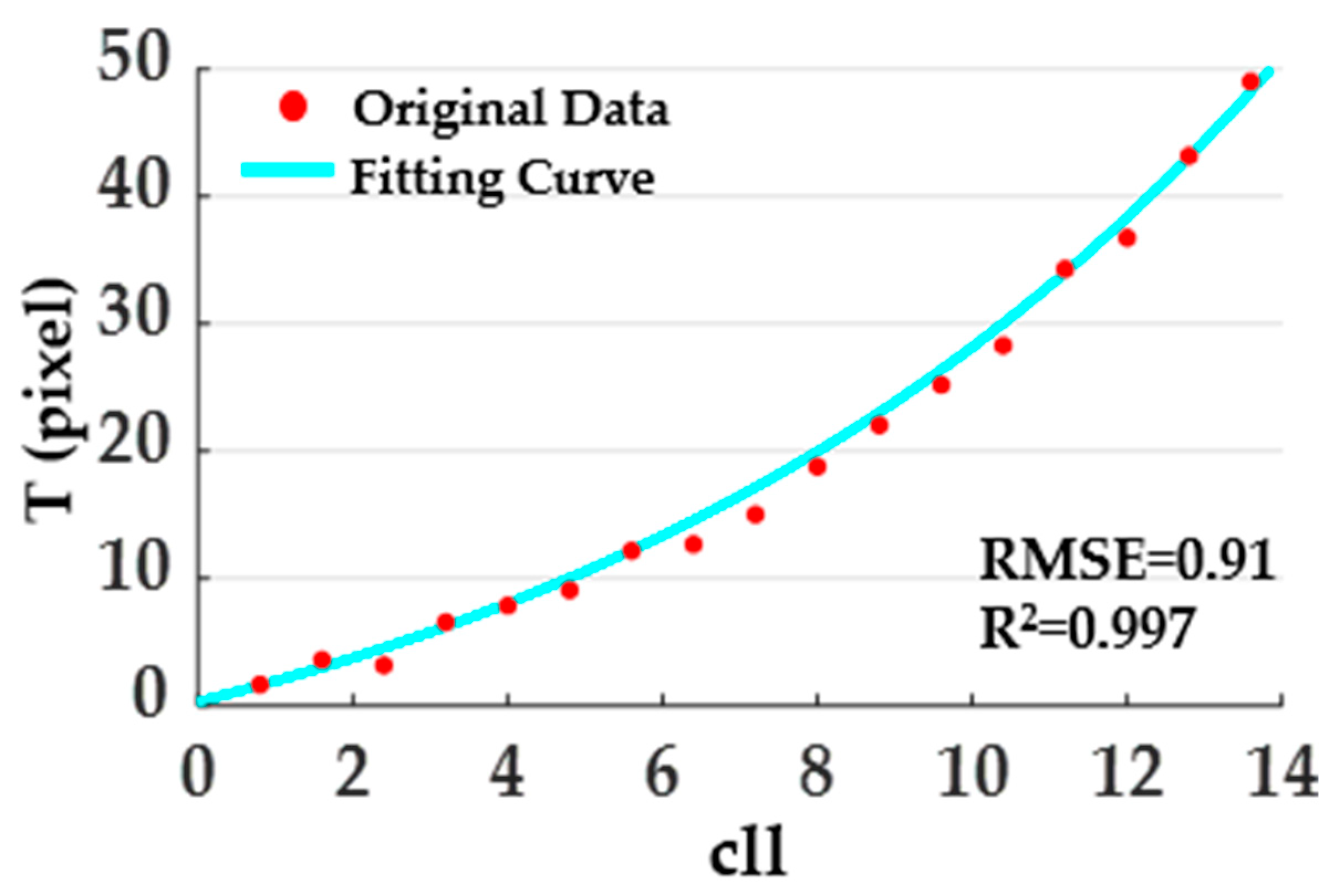
Gaussian fit

Surface correlation length is considered a measure of the height correlation between two points on a profile. In the theoretical model of image roughness, the common surface autocorrelation function has the Gaussian autocorrelation function [25]:

$$A{C}_{avg}=\exp (-\frac{{(d^{\prime })}^2}{cl{l}^2})$$

(7)

The surface correlation length $cll$ is defined as the interval $d^{\prime }$ when the autocorrelation function $A{C}_{avg}=1/e$. In general, the smaller the correlation length, the greater the image surface discrepancy.

(7)

Relationship between correlation length and period

Through numerical simulation, we simulated the value of BC of different periods, obtained the correlation length of the simulated value through (1)–(6), thereby fitting the relationship between the correlation length and the period (Equation (6)). The coefficient of determination is up to 0.997 (Figure 3).

$$T=14.29*\exp (0.1082*cll)-14.01$$

(8)

where $cll$ is the correlation length, and $T$ is the period. Using the above method, the period of BC noise on the time series of the four ground objects in the study area was calculated.

2.2.2. FFT Filtering Algorithm at Land Parcel Scale

The BFFT filtering method is implemented based on the available parcel boundary range, and the radar image is cropped according to the parcel boundary before filtering. The cropped image is BFFT filtered, and, finally, the filtered image is stitched back to the original image area. The specific steps of the BFFT filtering algorithm are as follows:

(1). A fast Fourier transform is done on the range of the parcel to convert the spatial domain image to the frequency domain image $S_{fre}$.

$$S_{fre}={\displaystyle \sum _{j=1}^m{\displaystyle \sum _{k=1}^n{e}^{-2\pi i(jp/m+kp/n)}{a}_{j,k}^{}}}$$

(9)

where $i$ is the imaginary unit, $p$ and $j$ are indices that run from 1 to $m$, and $q$ and $k$ are indices that run from 1 to $n$; $a_{j,k}$ is the value of the image at index ($j,k$)

(2). Calculate the noise period (T) according to Formula (8);

(3). The sampling frequency of known SAR images is $1/10$. In the frequency domain, the frequency corresponding to the position x from the DC component ($x$ starts from zero) is:

$$\omega =x*(Fs/n)$$

(10)

where $\omega$ represents the component frequency in the frequency domain, $Fs$ represents the sampling frequency of $1/10$, and $n$ represents the number of samples;

(4). The frequency of each component in the frequency domain is calculated using Equation 8. The noise frequency is obtained according to the noise period of different features. When the component’s frequency is greater than the frequency of the feature noise, it is considered that the noise has less influence on the SAR image. Therefore, this part of the component can be treated as noise, and noise removal can be performed using FFT low-pass filtering to reduce SAR image noise. In this article, considering the difference of mask shape, mask radius, and mask value on the effect, the Hann Window (Equation (12)) is used to generate the filter weight coefficient $\rho (D)$. Then, the mask is processed according to each frequency component’s distance to develop a new frequency domain component $H(u,v)$. The weight coefficient and value function are as follows:

$$\rho (D)=0.5*(1+\cos (2\pi \frac{D(u,v)}{R}))$$

(11)

$$H(u,v)=\{\begin{array}{l}h(u,v)\hfill \\ \rho (D)*h(u,v)\hfill \\ 0\hfill \end{array}\begin{array}{lll}\hfill & if\hfill & D(u,v)=0\hfill \\ \hfill & if\hfill & 0<D(u,v)\le R\hfill \\ \hfill & if\hfill & D(u,v)>R\hfill \end{array}$$

(12)

where $\rho (D)$ stands for the weight coefficient; $D(u,v)$ is the pixel distance from the DC component of each component in the frequency domain; $R$ Radius of the filter window. The magnitude of R is equal to the distance from the frequency component to the DC component when the frequency component’s frequency is equal to the noise cycle frequency. $H(u,v)$ is the value of the frequency domain component at the position $(u,v)$; $h(u,v)$ is the original value of the frequency domain image at the position $(u,v)$; $\rho (D)$ is the mask value function.

(5). Transforms the masked frequency domain image into a spatial domain image.

2.2.3. Filter Quality

The ability of various filtering methods to compare the mean value (AVE) to maintain the image radiation level and noise reduction was evaluated by comparing the BC values, standard deviation (STD), and equivalent vision (ENL) in the land parcel area before and after filtering [18]. The change in AVE represents changes in radiation levels, and STD represents the dispersion of the data. In contrast, ENL represents an indicator of regional smoothness, reflecting the magnitude of the noise reduction power of the filtering method.

When the SAR image is an intensity image, the equivalent vision (ENL) of the image is defined as:

$$\beta =\frac{\sqrt{\mathrm{var}(\widehat{x})}}{E(\widehat{x})}$$

(13)

$$ENL=1/{\beta }^2$$

(14)

where $\widehat{x}$ stands for the values of the filtered image BC. The larger the $ENL$ value, the better the filtering effect and the smoother the surface [26].

2.2.4. Comparison of Multiple Filtering Methods

In order to evaluate the capability of the BFFT filtering method, the Sentinel-1B images of the 22 July transit were processed for noise reduction using multiple filtering methods. According to the above calculation, the annual average noise period for different features at different polarizations is about 3.1 pixels (Figure 4). The BFFT filtering process is performed according to this noise period. The other six methods (Mean, Med, Lee, ReLee, Frost, NLM) were filtered using a filter window of 7 × 7 (pixel). After this, three evaluation parameters mentioned in Section 2.2.3 are used to evaluate the filtering effect. Furthermore, profile lines are used in the filtering result area to demonstrate further the magnitude of different filtering methods on the noise reduction capability of SAR images.

3. Results

3.1. Annual Analysis of Different Ground Object Noise Periods

Figure 4 is the annual variation characteristic of the BC noise period of VV and VH. The noise period change law of corn and soybean dryland crops was similar, with an apparent sudden increase in the noise period around day 120. In other stages, the annual difference of the polarization noise period was less than 0.15 pixels. The annual polarization noise period of paddy land parcels differs by 0.18 pixels. The water noise period varied significantly under different polarizations, except for days 71 and 95, when the noise period of VV polarization was larger than that of VH polarization. At around 90 days, the noise period is similar to the dryland crops, and around day 323, the VV band noise period is up to 4.5 pixels. Overall, the mean value of the noise period of the four ground objects with different polarizations fluctuated in the region of 3.1 pixels.

3.2. Comparison of the Effects of Multiple Filtering Methods

Appendix A shows the results of different filtering methods applied to different land parcels. The NLM and BFFT filtering results performed better. Still, using the NLM filtered images, the internal land parcel boundary area appeared to have a “dilation” (Figure A1-paddy-g\g’) or “erosion” (Figure A1-water-g\g’, corn-g) phenomenon. In areas with relatively high BC values, abnormal “high-value squares” appear after NLM filtering images (Figure A1-water-g’). BFFT can well retain the clarity of different ground boundary areas (Figure A1-paddy-h\h’) and can keep the “hole” area inside the land parcel (Figure A1-water-h\h’).

The mean value of BC was well maintained after filtering with different methods (Figure 5a,a’). The noise reduction effect of NLM and BFFT is noticeable, and the extent of dispersion of BC within the land parcel is reduced after filtering (Figure 5b,b’), with improved smoothness (Figure 5c,c’). The BFFT method has a better noise reduction effect on the water and paddy land parcels. After filtering, the dispersion degree of BC in the field is reduced to half of the original. (Paddy-VV), 0.005 (Paddy-VH) were reduced to 0.0016, 0.0002, 0.013, 0.002, and the smoothness was tripled, ENL was reduced from the original 2.65 (Water-VV), 3.55 (Water-VH), 3.34 (Paddy-VV), 3.25 (Paddy-VH) are increased to 12.87, 57.08, 13.95, 22.63. At the same time, NLM has a better noise reduction effect on soybean and corn land parcels. The degree of dispersion is reduced to one-third of the original STD from the original 0.052 (Corn-VV), 0.01 (Corn-VH), 0.052 (Soybean-VV), 0.013 (Soybean-VH) to 0.016, 0.002, 0.012, 0.003, and the smoothness increased by ten times. The ENL was increased from 5.54 (Corn-VV), 4.99 (Corn-VH), 5.76 (Soybean-VV), and 5.16 (soybean-VH) to 58.59, 85.98, 117.57, and 96, respectively.

Figure 6 indicates that the backscatter coefficient (red line) fluctuation is significantly reduced. The noise reduction effect of the NLM filtering method is pronounced on BC. The maximum peak difference of VV band BC decreased from 0.206 (Figure 6c) to 0.033, and the maximum peak difference of VH band BC decreased from 0.041 (Figure 6d’) to 0.006. At the same time, the BFFT method can reduce the fluctuation of BC within about a 6-pixel scale while preserving the fluctuation of BC on a large spatial scale.

3.3. Comparison of the Filtering Effects of the Time-Series Images

Figure 7 performs ENL statistics using different filtering methods. On the scale of the whole year, all the filtering methods contribute to the noise reduction effect. The noise reduction effect is evident in Med, BFFT, and NLM methods. Compared with other filtering methods, BFFT and Med have the best noise reduction effect on the water block (Figure 7), and the annual mean of ENL value improves from the original 3 (VV), and 3 (VH) up to 17 (BFFT-VV), 46 (BFFT-VH), 11 (Med-VV), and 29 (Med-VH). The NLM noise reduction effect is the most significant for paddy, corn, and soybean. The annual mean of the ENL of the three ground objects under VV polarization increases from 4, 5, and 5 to 39, 90, and 88. The annual mean of ENL under VH polarization increases from 3, 4, and 3 to 21, 51, and 40. It is worth noting that the BFFT filtering method has better stability when filtering the corresponding region of corn and soybean, two dryland crops. The extreme value difference on the ENL annual scale is significantly smaller than the value difference from the NLM method.

4. Discussion

4.1. The Filtering Method Based on the Land Parcel Boundary Improves the Boundary Blur Phenomenon of the Original Filtering Method

Figure 8 shows the difference between adjacent land parcels after using NLM and BFFT filtering methods, and both NLM and BFFT can reduce the noise of radar images very well. In the three regions (Figure 9–Soybean, Paddy_Q1, Paddy_Q2) (Figure 9c–e), BFFT can retain the changing trend of the original image profile (Origin line) in the land parcel while reducing the noise. In particular, significant attention is given to the enormous BC value on the radar image at the land parcel and the parcel’s junction (Figure 8–Avenue_Q1\Q2). When filtering by using The NLM filtering method, although the high-value fluctuation in this part of the region, it also makes the relatively low value of the junction (blue dotted line: blue dashed line) land parcel higher. When using BFFT filtering, since the filtering process is only performed on the inside of the land parcel, the avenue area between the land parcels does not participate in the filtering process, so the problem of boundary area dilation is well avoided. The BFFT filtering method maintains the clarity of the land parcel’s edge features while reducing the block’s internal noise (Figure 9g).

4.2. Filtering Effect Varies with the Change of the FFT Filter Radius and the Selection of the Optimal Filter Radius

Filter window size selection has a profound image-filtering effect. The BFFT filtering method used in this paper is based on the noise period and the land parcel size combined with the Hann Window. The larger the radius of the filter window, the more high-frequency components are contained, resulting in more pronounced speckle noise in the filtered image [27,28,29]. Select a region of 51 × 51 pixels within the Figure 1d’ area, and use the FFT filtering method to filter the VV polarization according to the size of different filter radii.

(a)–(h) in Figure 9 corresponds to the filtering results under different filtering radii. As the filtering radius decreases, the high-frequency information included becomes less, and the low-frequency information content increases until the scatter of the filtered image disappears (Figure 9h). It is worth noting that the differences in details between pixels in the original image are also erased with the disappearance of speckle noise. The NDVI (Figure 9i) distribution obtained from the simultaneous multispectral images of this region with a single crop planting shows that there are still differences in crop growth within the area, and such differences are also reflected in the numerical distribution of the SAR images. To explore the size of the optimal filtering window and further illustrate the rationality of the BFFT method, the filtering radius was incremented by a one-pixel step, and the filtered results were evaluated (Figure 10). Figure 11 shows the same pattern as Figure 10; with the increase of the filter radius, the ENL of the processed image becomes smaller, and the standard deviation of BC becomes larger. At the same time, the mean value of the filtered BC does not change regardless of the radius change, and the value remains stable, which is the advantage of the FFT method.

When using the BFFT method to filter the corresponding area of Figure 10, the size of the filtering radius is calculated to be 8.23 pixels. From the statistics of Figure 11, it can be seen that when the R is less than 8 pixels, the ENL value decreases rapidly, and the change rate is faster than 20 for each change, while when the radius change is greater than 8 pixels, the ENL change rate is slower, and the change value is less than 10. From the filtering effect, when the filter radius change is less than 8 pixels, each radius change has a greater degree of impact. From the ENL parameters and noise reduction effects of the above filtering results, the BFFT filtering method removes high-frequency noise while maximizing the retention of high-frequency components and low-frequency components in the frequency domain and preserving the variance characteristics within the parcel. The correctness of the BFFT method idea is further demonstrated.

4.3. BFFT Filter Method for Large Area

The speed of filtering in processing large areas is also an important criterion. The Sentinel-1B image of 22 July 2021 was selected to filter the radar image under VV polarization of the same area using both NLM and BFFT filtering methods.

The unprocessed SAR image (Figure 11c) contains 103 parcels (Figure 11b) and the boundaries of the parcels can be distinguished well, but there are apparent speckle noise features inside the parcels. Considering the image after filtering using the NLM filtering method (Figure 11d), although the speckle-noise features inside the parcels are reduced, the boundaries of different parcels appear blurred due to pixel dilation. The high-value areas corresponding to the SAR images (corresponding to the building areas) significantly impact the cultivated areas in the filtering (Figure 11q1). The noise reduction effect of the image after using BFFT filtering is the most outstanding (Figure 11e). Not only is the noise inside the plot better reduced, but the parcel’s boundary is also preserved. It is noteworthy that the boundaries of the differentiated areas within the parcels become more apparent after the BFFT filtering (Figure 11q2). This section compares the difference in processing time between the two filtering methods, NLM and BFFT. NLM’s processing time is 317.53 s, while the BFFT filtering method’s processing time is 0.36 s. Thus, the BFFT filtering method has certain advantages in terms of filtering effect and processing rate when dealing with a large area.

5. Conclusions

This paper proposes a SAR image FFT filtering method that integrates the spatial autocorrelation features of speckle noise and the block boundaries. The algorithm determines the size of the filter radius based on the periodic characteristics of noise within the range of specific ground objects and blocks. The selection based on the FFT filter radius has a theoretical basis.

The application scenario of the BFFT filtering method is based on the quantitative inversion of the target area in a large area of the SAR images, and the noise requirement in the non-target regions is relatively low. This paper compares seven commonly used filtering methods. From the perspective of evaluation parameters, NLM and BFFT have better noise reduction effects. While suppressing the noise, the BFFT method retains the changing trend of the internal values of the plot, the change transition is smoother, and the image processing speed is also faster.

In future work, we will consider the performance of SAR images at different resolutions when using the BFFT method and do a more in-depth study of the noise period at various resolutions. It is worth mentioning that the BFFT method also provides a new idea for noise reduction of multispectral images.

References

- Lee, J.-S. Speckle Suppression and Analysis for Synthetic Aperture Radar Images. Opt. Eng. 1986, 25, 636–643. [Google Scholar] [CrossRef]
- Liu, F.; Masouros, C.; Petropulu, A.P.; Griffiths, H.; Hanzo, L. Joint Radar and Communication Design: Applications, State-of-the-Art, and the Road Ahead. IEEE Trans. Commun. 2020, 68, 3834–3862. [Google Scholar] [CrossRef] [Green Version]
- Maity, A.; Pattanaik, A.; Sagnika, S.; Pani, S. A Comparative Study on Approaches to Speckle Noise Reduction in Images. In Proceedings of the 1st International Conference on Computational Intelligence and Networks (CINE 2015), Bhubaneswar, India, 12–13 January 2015; pp. 148–155. [Google Scholar] [CrossRef]
- López-Martínez, C.; Fàbregas, X. Polarimetric SAR Speckle Noise Model. IEEE Trans. Geosci. Remote Sens. 2003, 41, 2232–2242. [Google Scholar] [CrossRef] [Green Version]
- Qiu, F.; Berglund, J.; Jensen, J.R.; Thakkar, P.; Ren, D. Speckle Noise Reduction in SAR Imagery Using a Local Adaptive Median Filter. Gisci. Remote Sens. 2004, 41, 244–266. [Google Scholar] [CrossRef] [Green Version]
- Ma, X.; Wu, P.; Wu, Y.; Shen, H. A Review on Recent Developments in Fully Polarimetric SAR Image Despeckling. IEEE J. Sel. Top. Appl. Earth Obs. Remote Sens. 2018, 11, 743–758. [Google Scholar] [CrossRef]
- Wu, W.; Huang, X.; Shao, Z.; Teng, J.; Li, D. SAR-DRDNet: A SAR Image Despeckling Network with Detail Recovery. Neurocomputing 2022, 493, 253–267. [Google Scholar] [CrossRef]
- Baraha, S.; Sahoo, A.K.; Modalavalasa, S. A Systematic Review on Recent Developments in Nonlocal and Variational Methods for SAR Image Despeckling. Signal Process. 2022, 196, 108521. [Google Scholar] [CrossRef]
- Foucher, S.; Farage, G.; Bénié, G.B. Polarimetric SAR Image Filtering with Trace-Based Partial Differential Equations. Can. J. Remote Sens. 2014, 33, 226–236. [Google Scholar] [CrossRef]
- Chan, D.; Gambini, J.; Frery, A.C. Entropy-Based Non-Local Means Filter for Single-Look SAR Speckle Reduction. Remote Sens. 2022, 14, 509. [Google Scholar] [CrossRef]
- Pang, Y.; Jiang, S.; Cheng, B.; Liu, W.; Wu, Y. Design and Implement of Median Filter toward Remote Sensing Images Based on FPGA. In Proceedings of the International Conference on ASIC, Kunming, China, 26–29 October 2021. [Google Scholar] [CrossRef]
- Yommy, A.S.; Liu, R.; Onuh, S.O.; Ikechukwu, A.C. SAR Image Despeckling and Compression Using K-Nearest Neighbour Based Lee Filter and Wavelet. In Proceedings of the 2015 8th International Congress on Image and Signal Processing (CISP 2015), Shenyang, China, 14–16 October 2015; pp. 158–167. [Google Scholar] [CrossRef]
- Sun, Z.; Zhang, Z.; Chen, Y.; Liu, S.; Song, Y. Frost Filtering Algorithm of SAR Images with Adaptive Windowing and Adaptive Tuning Factor. IEEE Geosci. Remote Sens. Lett. 2020, 17, 1097–1101. [Google Scholar] [CrossRef]
- Quegan, S.; Yu, J.J. Filtering of Multichannel SAR Images. IEEE Trans. Geosci. Remote Sens. 2001, 39, 2373–2379. [Google Scholar] [CrossRef]
- Lattari, F.; Leon, B.G.; Asaro, F.; Rucci, A.; Prati, C.; Matteucci, M. Deep Learning for SAR Image Despeckling. Remote Sens. 2019, 11, 1532. [Google Scholar] [CrossRef] [Green Version]
- Franceschetti, G.; Schirinzi, G. A SAR Processor Based on Two-Dimensional FFT Codes. IEEE Trans. Aerosp. Electron. Syst. 1990, 26, 356–366. [Google Scholar] [CrossRef]
- Weaver, J.B.; Xu, Y.; Healy, D.M.; Cromwell, L.D. Filtering Noise from Images with Wavelet Transforms. Magn. Reson. Med. 1991, 21, 288–295. [Google Scholar] [CrossRef]
- Dong, Y.; Milne, A.K.; Forster, B.C. Toward Edge Sharpening: A SAR Speckle Filtering Algorithm. IEEE Trans. Geosci. Remote Sens. 2001, 39, 851–863. [Google Scholar] [CrossRef]
- Simard, M.; Degrandi, G. Analysis of Speckle Noise Contribution on Wavelet Decomposition of SAR Images. IEEE Trans. Geosci. Remote Sens. 1998, 36, 1953–1962. [Google Scholar] [CrossRef]
- Sentinel-1—Overview—Sentinel Online—Sentinel Online. Available online: https://sentinels.copernicus.eu/web/sentinel/missions/sentinel-1/overview (accessed on 18 December 2022).
- Sentinel-1 Toolbox—Sentinel Online. Available online: https://sentinel.esa.int/web/sentinel/toolboxes/sentinel-1 (accessed on 2 October 2022).
- Durand, S.; Fadili, J.; Nikolova, M. Multiplicative Noise Cleaning via a Variational Method Involving Curvelet Coefficients. In Scale Space and Variational Methods in Computer Vision; Lecture Notes in Computer Science (Including Subseries Lecture Notes in Artificial Intelligence and Lecture Notes in Bioinformatics); Springer: Berlin/Heidelberg, Germany, 2009; Volume 5567, pp. 282–294. [Google Scholar] [CrossRef]
- Salehi, H.; Vahidi, J.; Abdeljawad, T.; Khan, A.; Rad, S.Y.B. A SAR Image Despeckling Method Based on an Extended Adaptive Wiener Filter and Extended Guided Filter. Remote Sens. 2020, 12, 2371. [Google Scholar] [CrossRef]
- Marcoleonetti1 (2022). Speckle Autocorrelation—File Exchange—MATLAB Central. Available online: https://ww2.mathworks.cn/matlabcentral/fileexchange/94765-speckle-autocorrelation?s_tid=srchtitle_speckle%20autocorrelation_1 (accessed on 2 October 2022).
- Maes, M.A.; Breitung, K.; Dann, M.R. At Issue: The Gaussian Autocorrelation Function. Lect. Notes Civil Eng. 2021, 153 LNCE, 191–203. [Google Scholar] [CrossRef]
- Li, H.; Duan, X.L. SAR Ship Image Speckle Noise Suppression Algorithm Based on Adaptive Bilateral Filter. Wirel. Commun. Mob. Comput. 2022, 2022, 9392648. [Google Scholar] [CrossRef]
- Rubel, O.; Lukin, V.; Rubel, A.; Egiazarian, K. Selection of Lee Filter Window Size Based on Despeckling Efficiency Prediction for Sentinel SAR Images. Remote Sens. 2021, 13, 1887. [Google Scholar] [CrossRef]
- Irfan Shaikh, A.; Shafiyoddin Badroddin, S. Statistical Analysis of Speckle Noise Reduction in C-Band SAR Image Using FFT Based Circular Pass Filter And Circular Cut Filter. Ann. Rom. Soc. Cell Biol. 2021, 25, 1054–1065. [Google Scholar]
- Mateo, C.; Talavera, J.A. Short-Time Fourier Transform with the Window Size Fixed in the Frequency Domain (STFT-FD): Implementation. SoftwareX 2018, 8, 5–8. [Google Scholar] [CrossRef]
Disclaimer/Publisher’s Note: The statements, opinions and data contained in all publications are solely those of the individual author(s) and contributor(s) and not of MDPI and/or the editor(s). MDPI and/or the editor(s) disclaim responsibility for any injury to people or property resulting from any ideas, methods, instructions or products referred to in the content. |
© 2022 by the authors. Licensee MDPI, Basel, Switzerland. This article is an open access article distributed under the terms and conditions of the Creative Commons Attribution (CC BY) license (https://creativecommons.org/licenses/by/4.0/).
Share and Cite
Wang, X.; Meng, Z.; Chen, S.; Feng, Z.; Li, X.; Guo, T.; Wang, C.; Zheng, X. A Block-Scale FFT Filter Based on Spatial Autocorrelation Features of Speckle Noise in SAR Image. Remote Sens. 2023, 15, 247. https://doi.org/10.3390/rs15010247
Wang X, Meng Z, Chen S, Feng Z, Li X, Guo T, Wang C, Zheng X. A Block-Scale FFT Filter Based on Spatial Autocorrelation Features of Speckle Noise in SAR Image. Remote Sensing. 2023; 15(1):247. https://doi.org/10.3390/rs15010247
Chicago/Turabian StyleWang, Xigang, Zhiguo Meng, Si Chen, Zhuangzhuang Feng, Xinbiao Li, Tianhao Guo, Chunmei Wang, and Xingming Zheng. 2023. "A Block-Scale FFT Filter Based on Spatial Autocorrelation Features of Speckle Noise in SAR Image" Remote Sensing 15, no. 1: 247. https://doi.org/10.3390/rs15010247