NRN-RSSEG: A Deep Neural Network Model for Combating Label Noise in Semantic Segmentation of Remote Sensing Images

Abstract

The performance of deep neural networks depends on the accuracy of labeled samples, as they usually contain label noise. This study examines the semantic segmentation of remote sensing images that include label noise and proposes an anti-label-noise network framework, termed Labeled Noise Robust Network in Remote Sensing Image Semantic Segmentation (NRN-RSSEG), to combat label noise. The algorithm combines three main components: network, attention mechanism, and a noise-robust loss function. Three different noise rates (containing both symmetric and asymmetric noise) were simulated to test the noise resistance of the network. Validation was performed in the Vaihingen region of the ISPRS Vaihingen 2D semantic labeling dataset, and the performance of the network was evaluated by comparing the NRN-RSSEG with the original U-Net model. The results show that NRN-RSSEG maintains a high accuracy on both clean and noisy datasets. Specifically, NRN-RSSEG outperforms UNET in terms of PA, MPA, Kappa, Mean_F1, and FWIoU in the presence of noisy datasets, and as the noise rate increases, each performance of UNET shows a decreasing trend while the performance of NRN-RSSEG decreases slowly and some performances show an increasing trend. At a noise rate of 0.5, the PA (−6.14%), MPA (−4.27%) Kappa (−8.55%), Mean_F1 (−5.11%), and FWIOU (−9.75%) of UNET degrade faster; while the PA (−2.51%), Kappa (−3.33%), and FWIoU of NRN-RSSEG (−3.26) degraded more slowly, MPA (+1.41) and Mean_F1 (+2.69%) showed an increasing trend. Furthermore, comparing the proposed model with the baseline method, the results demonstrate that the proposed NRN-RSSEG anti-noise framework can effectively help the current segmentation model to overcome the adverse effects of noisy label training.

1. Introduction

Traditional methods for semantic segmentation of remote sensing images mainly decode remote sensing feature information by means of texture, edge, spectrum, length, and other information [1,2,3]. With the rapid development of deep learning [4,5,6], convolutional neural networks (CNNs) are widely used in the semantic segmentation of remote sensing images [7,8,9,10,11]. However, manually produced sample labels inevitably contain some errors, called label noise, which reduces the models’ predictive ability [12,13,14] while increasing the number of training features and model complexity [15]. Sample learning with label noise is an ongoing problem in deep learning.

Current algorithms on label noise research follow three main categories: noise transfer matrix [16], data-based [17,18], and loss function-based [19,20]. Noise transfer matrix approaches employ the concept of modeling against label noise. Sukhbaatar et al. [16] embedded a known noise transfer matrix (confusion matrix) into a loss function. This is a Bayesian-based approach that treats the correct labels as latent variables, and because the noise transfer matrix is known when the training stage is complete, removing the noise transfer matrix yields the predicted labels. However, in practice, the true noise transfer matrix is unknown. Subsequently, several studies have estimated the noise transfer matrix [21,22,23]. However, the larger the number of categories, the more difficult the exact estimation is to achieve, and the noise transfer matrix approach is only applicable to asymmetric noise labels but not symmetric noise.

Data-based label noise learning algorithms focus on removing noisy samples or reducing the impact of noisy samples on the model through certain mechanisms. Sample reweighting is representative of this type of algorithm, which identifies samples suspected of being mislabeled based on information, such as sample loss values [17,24,25], sample probabilities of model output [18,26,27], and gradients [28,29,30], and then eliminates the suspected mislabeled samples by assigning low weights. Northcutt et al. [27] proposed a confidence learning framework based on three main steps. First, evaluating the joint distribution of the noisy and true labels of the samples, then identifying mislabeled samples, and finally, reweighting and re-adding the samples to the training after screening out the mislabeled samples. Under sufficiently realistic conditions, the confidence learning framework can accurately detect label errors and estimate the joint distribution of noisy and true labels. However, this approach relies heavily on the model’s performance with noisy learning and requires reasonable fine-tuning of the superparameters. Ren et al. [31] proposed a reweighting algorithm in the case of additional clean, unbiased validation sets without adjusting the superparameters. In each training iteration, the samples were reweighted according to the similarity of the fall direction of the validation loss plane by examining the fall direction of some of the training samples on the training loss plane. Pham et al. [32] proposed a meta-pseudo-labeling algorithm that treats suspected noisy sample data in training data as unlabeled data for semi-supervised learning. However, biases in sample selection may lead to error accumulation.

Loss function-based learning algorithms reduce the impact of noisy labels by reducing the value of losses during training. Numerous studies have shown that the processing of the loss function leads to better robustness of the label noise during training [19,20,33,34,35]. Such methods can reduce the impact of erroneous samples by designing a robust loss function. The cross-entropy loss (CE) function [33] is commonly used for classification, providing fast convergence yet easy fitting of noisy samples, but it has poor generalization ability. Ghosh et al. [33] demonstrated that the symmetric loss function can robustly label noise. The mean absolute error (MAE) [19] derived under this design principle has good robustness in experimental results under multiple classification labels but will underfit on complex datasets. In addition, Feng et al. [20] designed a Taylor cross entropy (TCE) loss based on CE inspired by the Taylor function. In that approach, TCE approximates CE by adjusting the hyperparameters indirectly to adjust the Taylor rank, which not only inherits the advantages of CE but also avoids the disadvantages of CE overfitting and is more resilient to label noise than CE.

In the case of massive remote sensing images, the development of image segmentation methods that allow machines to tolerate a certain amount of label noise has become an urgent problem. We therefore propose a labeled noise robust network (NRN-RSSEG) to suppress the effect of label noise when conducting semantic segmentation of remote sensing images. The proposed algorithm combines the attention mechanism with a noise-robust loss function. The algorithm was evaluated using the Vaihingen region of the ISPRS Vaihingen 2D Semantic Labeling dataset, and the results were compared with the original classification network approach. The main contributions of this study are as follows. (1) A general network framework is proposed, whose attention mechanism and noise-robust loss function can be applied to other classification networks as submodules with the advantage of plug-and-play; (2) three different noise rates and two different types of noise (symmetric labeling noise and asymmetric labeling noise) are considered, and the results show that the algorithm is able to maintain high accuracy and good generalization performance under different noise rates and noise types.

2. Datasets and Methods

2.1. Dataset

ISPRS Vaihingen 2D Semantic Labeling [36] is an ultra-high-resolution airborne remote sensing semantic labeling dataset, from which the Vaihingen region dataset was selected for model evaluation in this study (https://www.isprs.org/education/benchmarks/UrbanSemLab/default.aspx; accessed on 20 March, 2022). The dataset mainly consisted of NIR, red, and green channels with corresponding surface elevation models and standardized surface elevation data. The dataset includes six feature types: impervious surfaces, buildings, low vegetation, trees, cars, and other categories (clutter/background) (Figure 1).

2.2. Experimental Design

Pixel-level remote sensing land-cover tagging typically encounters two types of error: contamination by symmetric and asymmetric label noise. Symmetric label noise occurs when real labels are contaminated with the same probability as other labels, and asymmetric label noise occurs when real labels are flipped to specific wrong labels with fixed rules (Figure 2). Suppose the image is divided into $k$ classes, let $X\subset R^d$ be the feature space of the image and $Y=\left\{1,2,\cdots ,k\right\}$ be the label space. If there are $n$ training samples, where each $\left(x_i,y_i\right)\in \left(X\times Y\right)$ and $y_i$ is the correct label of $x_i$, then when contaminated by noise (noise rate $\phi \in \left(0,1\right)$), the set of correct labels $\left\{y_i\right\}$ degenerates to the set of noisy labels $\left\{y_i^{*}\right\}$. Consequently, there are $\phi \ast n$ samples assigned with incorrect labels, and the remaining $\left(1-\phi \right)n$ samples are clean samples. In practical tasks, the training set typically contains mixed types of label noise (both symmetric and asymmetric). To simulate this situation, these two types of noise were injected into the training set in equal proportions. Assuming $\phi =0.5$, this contains both 25% symmetric and 25% asymmetric noises. In this study, we tested three noise rates, setting $\phi$ to 0.3, 0.4, and 0.5.

For this dataset, Figure 2a shows the symmetric noise model. Assuming that a label is contaminated, it may be mislabeled as any other category with the same probability, and the grayscale values are consistent, indicating equal probability. Figure 2b is the asymmetric noise model; assuming that a label is contaminated, it is only mapped incorrectly into another class (indicated by white squares).

The dataset was divided into three parts: a training set containing label noise, test set, and validation set. For the Vaihingen dataset, nine images were used for training, four for testing, and three for validation. The original data were cropped to a size of 512 × 512 and fed into the deep neural network after horizontal and vertical flipping. The experimental GPU environment was RTX A4000, and TensorFlow (https://github.com/tensorflow/tensorflow, accessed on 3 April 2022) was used as the deep learning framework.

2.3. Methods

2.3.1. Network Structure

In this study, we designed an NRN-RSSEG that uses an attention mechanism [37] and a modified cross-entropy loss function to counteract the effect of label noise on model performance. The main network architecture of the NRN-RSSEG is built using the UNET model [38], the attention mechanism uses the Convolutional Block Attention Module (CBAM) [39], and the modified loss function is presented in Section 2.3.3. The model first passes the feature maps of the contraction paths in the Unet network through an attention mechanism and then splices them with the feature maps of the expansion paths. The introduction of an attention mechanism to the model is beneficial for enhancing the weight of image edges and suppressing secondary information, which in turn improves the segmentation effect of the model. The network structure is shown in Figure 3.

2.3.2. Attention Network

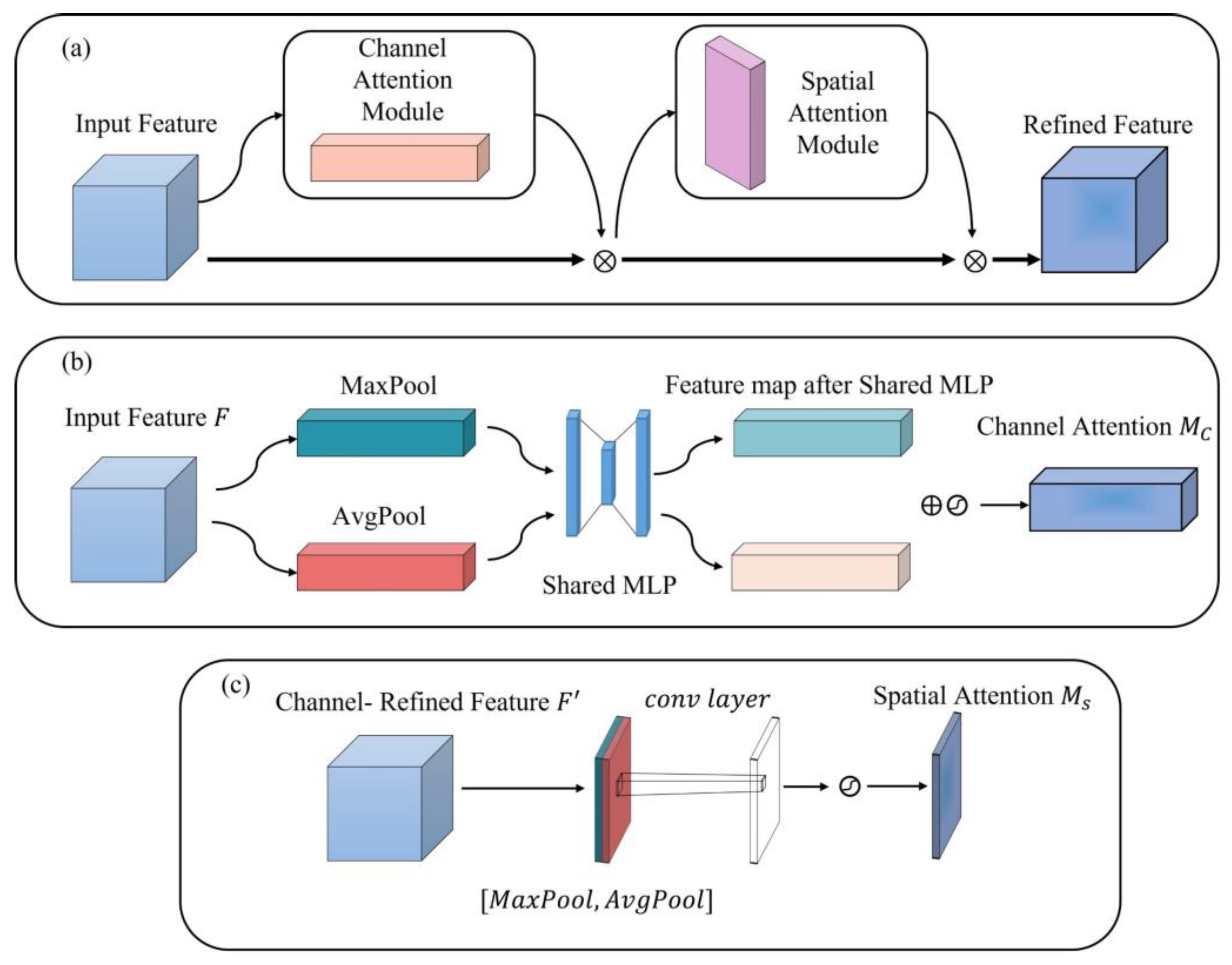
The attention mechanism is a method used in computer vision that focuses attention on important regions of an image and discards irrelevant information [37]. Attention mechanisms can be viewed as a dynamic process of selecting important information contained in image inputs, in the same way that humans distinguish between objects and classes. This process was implemented through adaptive feature weighting, by which we attempted to focus the model on important information and thus reduce the model’s fitting to noisy information. The Convolutional Block Attention Module (CBAM) is a lightweight attention module [39], schematically illustrated in Figure 4.

The CBAM was divided into a channel attention module and a spatial attention module. The input feature map was first point-multiplied by the channel attention value, then point-multiplied with the spatial attention module, and finally processed by CBAM to obtain the final feature map. The CBAM is defined as

$$F^{\prime }=M_C\left(F\right)\cdot F$$

(1)

$$F^{″}=M_C\left(F^{\prime }\right)\cdot F^{\prime }$$

(2)

where $M_C\left(F\right)$ is the channel attention module, $M_C\left(F^{\prime }\right)$ is the spatial attention module, $F$ is the input feature map, $F^{\prime }$ is the output of the channel attention module (i.e., the input of the spatial attention module), and $F^{″}$ is the output of the spatial attention module.

The channel attention module, also known as the feature attention module, first pooled the input feature map F by the maximum value and the average value to obtain two feature maps. Average pooling had feedback for each pixel point on the feature map, which was used to obtain global contextual information and could combine all information on the feature map to make corresponding decisions while maximum pooling had feedback for gradients when performing gradient back-propagation calculations, where only the largest response in the feature map had gradients, which can remove noise contained in the image and information unrelated to the target processing. The optimal results could be achieved by choosing average pooling and maximum pooling in the channel attention mechanism [39]. Second, the two feature maps were input to a multilayer perceptron (MLP) at the same time to perform dimensionality reduction and dimensionality enhancement operations, and the weights of the MLP were shared in this process. Finally, the two feature map outputs from the MLP were subjected to a summation operation and processed by the sigmoid function to obtain channel attention. The channel attention module is defined as follows:

$$M_C\left(F\right)=\sigma \left(MLP\left(AvgPool\left(F\right)\right)+MLP\left(MaxPool\left(F\right)\right)\right)$$

(3)

where $M_C\left(F\right)$ is the channel attention module, $\sigma$ is the sigmoid activation function, $MLP()$ is the multilayer perceptron, and $AvgPool()$ and $MaxPool()$ are the average pooling layer and maximum pooling layer, respectively.

The spatial attention module mainly responds to the importance of input values in the spatial dimension. First, the input values are pooled by the maximum and average values and then spliced. Second, the convolutional network is used to reduce the dimensionality to one channel, and finally, the sigmoid activation function obtains the output of this module. The spatial attention module can be defined as follows:

$$M_C\left(F^{\prime }\right)=\sigma \left(f\left[AvgPool\left(F^{\prime }\right);MaxPool\left(F^{\prime }\right)\right]\right)$$

(4)

where $M_C\left(F^{\prime }\right)$ is the spatial attention module and $f$ is the convolutional layer operation.

2.3.3. Modified Loss Function

In information theory, the Kullback–Leibler divergence is used to help measure the amount of information lost in the choice of approximation. Given the true distribution $q$ and approximate distribution $p$, the cross-entropy loss function can be expressed as $H\left(q,p\right)$, and the Kullback–Leibler function can be defined as

$$KL(q|\left|p\right)=H\left(q,p\right)-H\left(q\right)$$

(5)

where $H\left(q\right)$ is the entropy of q. In the semantic segmentation of remote sensing images, $q=q(k|x)$ and $p=p(k|x)$ were the distributions of the true and predicted labels, respectively. From the Kullback–Leibler perspective, the purpose of semantic segmentation is to minimize the difference between the true distribution $q$ and the predicted distribution $p$. However, when the semantic segmentation dataset contains label noise, $q(k|x)$ does not represent the true distribution; on the contrary, $p(k|x)$ can reflect the true distribution to some extent. Therefore, in addition to considering $q(k|x)$ as the underlying true value distribution, we also considered another direction of the Kullback–Leibler divergence, namely $KL(p|\left|q\right)$, to penalize the noisy samples, which can be defined as

$$SKL=KL(q|\left|p\right)+KL(p|\left|q\right)$$

(6)

Extending this idea to the cross-entropy loss function, we obtained the symmetric cross-entropy (SCE):

$$SCE=CE+RCE=H\left(q,p\right)+H\left(p,q\right)$$

(7)

where $CE$ is the cross-entropy loss function and $RCE$ is the reverse cross-entropy loss function. Although $RCE$ had good noise robustness [40], its convergence rate was slow, and for more effective and robust learning, we used two hyperparameters, $\alpha$ and $\beta$. $\alpha$ was used to control the overfitting of $CE$ to noisy samples, and $\beta$ controlled the model to be more robust to noisy samples. Thus, the final loss function form is defined as:

$$loss=\alpha \ast CE+\beta \ast RCE$$

(8)

To balance convergence speed and robustness, $\alpha$ was set to 0.1 and $\beta$ was set to 1 when the noise rates were 0% and 30%, and $\alpha$ was set to 0.01 and $\beta$ to 1 when the noise rates were 40% and 50%.

2.3.4. Sliding Window Prediction

Remote sensing images are usually very large, such that current hardware resources cannot infer an entire image simultaneously. Consequently, the conventional inference strategy is to divide the large image into fixed-size image blocks from left to right and from top to bottom and to use the model to infer these image blocks separately to obtain the inferred label map of each image block. These smaller label maps are then stitched together to form the final label map of the entire scene. However, using conventional regular grid cropping followed by prediction stitching, the edge region of each image block contains less contextual information; therefore, the resulting prediction is less accurate, which in turn also leads to evident stitching traces.

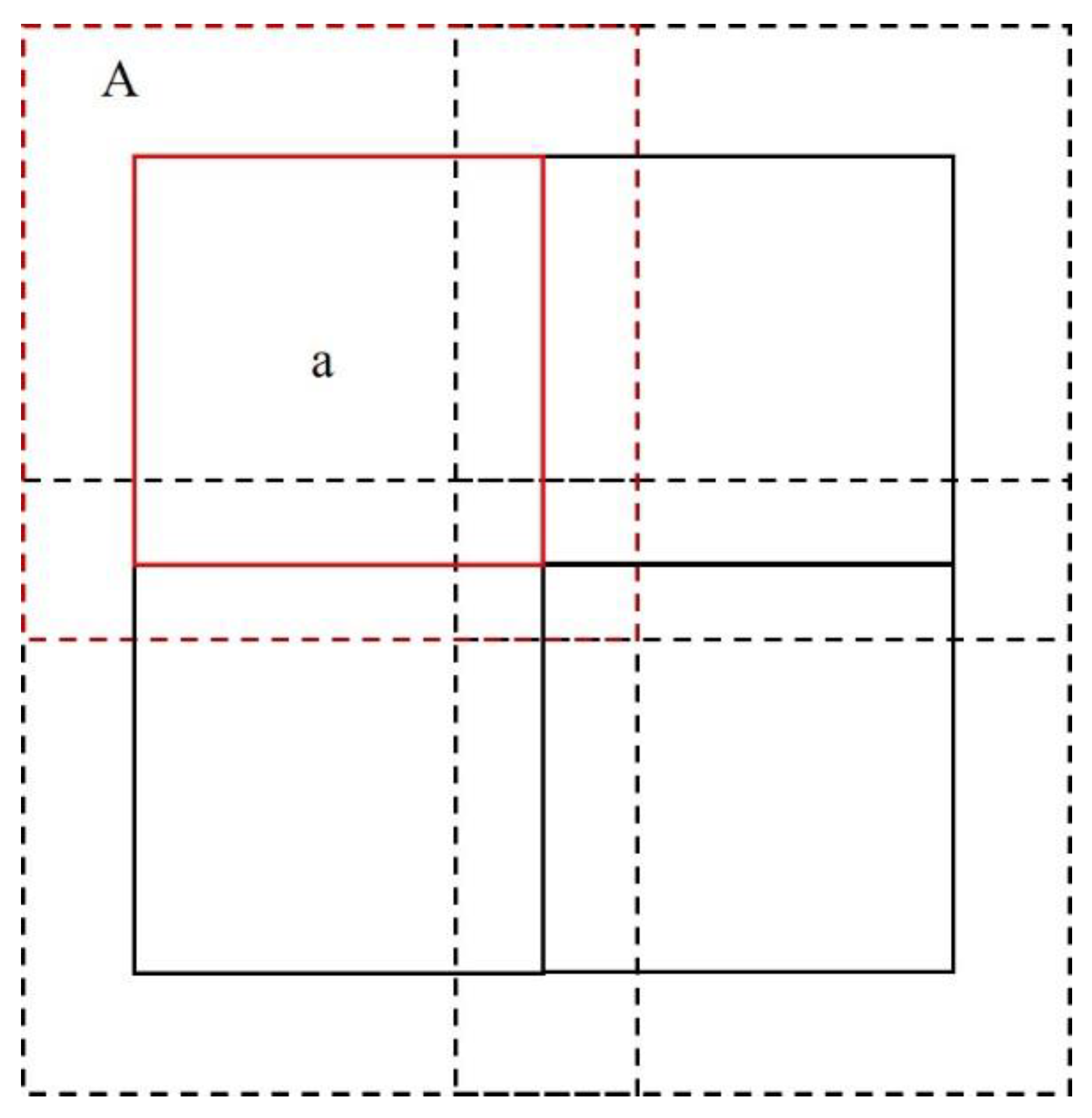
We used “ignore edge” prediction [41] (i.e., cropping images with overlap and adopting the “ignore edge” strategy in stitching as shown in Figure 5), where the actual cropped image was predicted as $\mathrm{A}$, the result of performing stitching was $\mathrm{a}$, the percentage of $\mathrm{a}$ to the region of $\mathrm{A}$ was $\mathrm{r}$, and the overlap ratio of neighboring cropped images was $1-\sqrt{\mathrm{r}}$.

2.3.5. Assessment

In this study, pixel accuracy (PA), category mean pixel accuracy (MPA), kappa coefficient (Kappa), F1 score (F1), and frequency-weighted intersection over union (FWIoU) were used to evaluate the proposed model.

Pixel accuracy is the ratio of the number of correct samples to the total number of samples, and in remote sensing image segmentation tasks, it refers to the ratio of the number of correctly classified pixels to the total number of pixels. Pixel accuracy is defined as

$$PA=\frac{TP+TN}{TP+TN+FP+FN}$$

(9)

where $PA$ represents the pixel accuracy, $P$ represents the number of positive class samples, and $N$ represents the number of negative class samples. True positive ($TP$) represents the number of positive class samples correctly classified by the model, and true negative ($TN$) represents the number of negative class samples correctly classified by the classification model. $FP$ represents the number of false positive samples (i.e., the number of positive classes that should have been negative) and $FN$ represents the number of false negative samples (i.e., the number of negative classes that should have been positive).

For Category Mean Pixel Accuracy (MPA), the proportion of pixels correctly classified for each class was calculated separately and then averaged as follows:

$$MPA=\frac{TP}{TP+FP}$$

(10)

The kappa coefficient (Kappa) is a consistency test that measures the effectiveness of a classification. For the semantic segmentation task of remote sensing images, the consistency is whether the model predicts the same result as the actual result. The kappa coefficient was calculated based on the confusion matrix, which took values between −1 and 1, usually greater than 0. Kappa is defined as

$$Kappa=\frac{p_o-p_e}{1-p_e}$$

(11)

where $p_o$ is the pixel precision (PA). Suppose the number of real samples in each class is a₁, a₂, …, a_n, the predicted number of samples in each category is b₁, b₂, …, b_n, then $p_e$ is defined as

$$p_e=\frac{a_1\ast b_1+a_2\ast b_2+\cdots +a_n\ast b_n}{n^2}$$

(12)

Recall is the probability of a positive sample being predicted in a sample that is actually positive. Recall is defined as

$$Recall=\frac{TP}{TP+FN}$$

(13)

The F1 score (F1) takes into account both the MPA and Recall of the classification model, and the F1 score can be regarded as a kind of reconciled average of the model MPA and Recall. F1 is defined as

$$F1=2 \frac{Recall\ast MPA}{Recall+MPA}$$

(14)

$$Mean\text{\_}F1={\displaystyle \sum }_i^{N-1}\frac{F1}{N}$$

(15)

Frequency weighted intersection over union (FWIoU) is an important measure of segmentation accuracy in image segmentation [42]. It is based on the frequency of each class and is multiplied by the intersection over union (IoU) of each class and summed. FWIoU is defined as

$$FWIoU=\frac{TP+FN}{TP+FP+TN+FN}\ast \frac{TP}{\left(TP+FP+FN\right)}$$

(16)

3. Results

3.1. Sample Performance

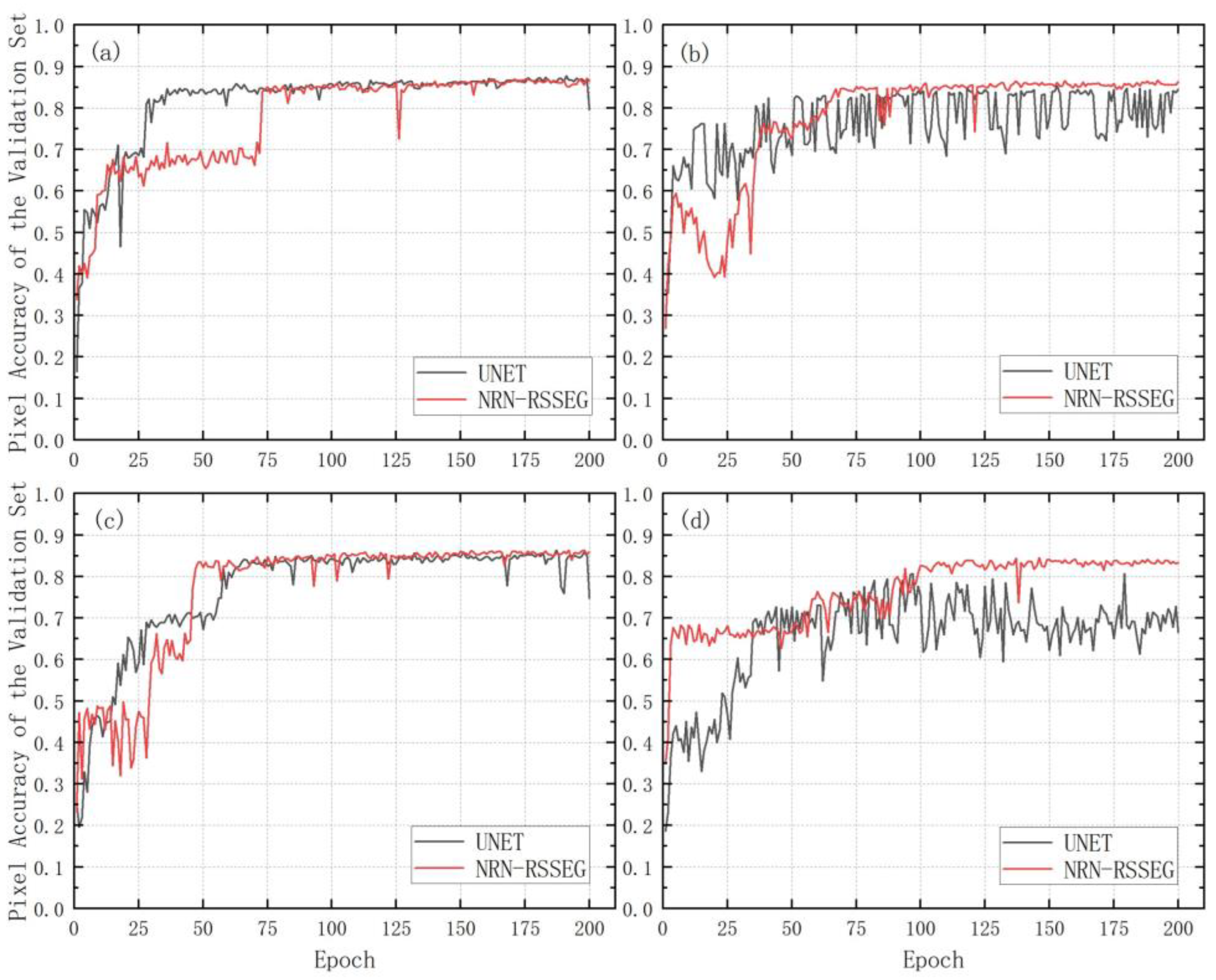
In this study, 30%, 40%, and 50% of the mixed label noise was injected into the original dataset. These were used to simulate the symmetric and asymmetric label noise introduced in the annotation process and also tested on a clean sample set ($\phi =0$). In this experiment, five metrics, PA, MPA, Kappa, Mean_F1, and FWIoU, were used to evaluate UNET and NRN-RSSEG. The results are shown in

Table 1. Test results of UNET and NRN-RSSEG, bold represents the high value of this assessment index at the same noise rate. (φ = noise rate).

Meath	Assessment	$\mathit{\phi }=0$	$\mathit{\phi }=0.3$	$\mathit{\phi }=0.4$	$\mathit{\phi }=0.5$
UNET	PA	0.8288	0.8097	0.8208	0.7674
	MPA	0.8217	0.8070	0.8284	0.7790
	Kappa	0.7729	0.7455	0.7610	0.6874
	Mean_F1	0.8019	0.8056	0.7277	0.7508
	FWIoU	0.7145	0.6813	0.7007	0.6170
NRN-RSSEG	PA	0.8309	0.8288	0.8287	0.8058
	MPA	0.7935	0.8312	0.8285	0.8076
	Kappa	0.7752	0.7720	0.7722	0.7419
	Mean_F1	0.7873	0.8286	0.8296	0.8082
	FWIoU	0.7157	0.7140	0.7151	0.6831

, and the training process is shown in Figure 6.

From the test results, we can see that both UNET and NRN-RSSEG can maintain high accuracy on clean datasets ($\phi =0$); NRN-RSSEG can also show better prediction on clean datasets, and all the performances metrics for UNET show a significant decreasing trend with increasing noise rate. In particular, at 50% noise rate, PA decreased by 6.14%, MPA by 4.27%, Kappa by 8.55%, Mean_F1 by 5.11%, and FWIoU by 9.75%. In comparison, NRN-RSSEG showed no significant decreasing trend in each performance and maintained good noise robustness. Comparing the performance of the two models at the same noise rate, NRN-RSSEG outperformed UNET when noise was present in the labels: NRN-RSSEG showed higher PA (1.91%), MPA (2.42%), Kappa(2.65%), Mean_F1(2.30%), and FWIoU (3.27%) than UNET at a noise rate of 0.3 and also higher PA (0.79%), MPA (0.01%), Kappa(1.12%), Mean_F1(10.19%), and FWIoU (1.44%) at a noise rate of 0.4. Our experimental results show that when the noise rate reaches a certain level, there is a positive feedback effect and the performance of both models improves. When the noise rate reached 0.5, the performance of UNET decreased significantly, with the result that the PA of NRN-RSSEG was significantly higher than those of UNET (3.84%), MPA (2.86%),Kappa(5.54%), Mean_F1(5.74%), and FWIoU (6.61%).

Figure 6 shows the pixel accuracy curves for the two models using the test dataset with different noise rates. Figure 6a shows that on the clean sample set, UNET converges quickly after 27 epochs, whereas NRN-RSSEG converges only after 75 epochs. At a noise rate of 30% (Figure 6b), the pixel accuracy curve of UNET oscillates more than that of NRN-RSSEG, which indicates that the label noise has some influence on UNET, and at the later stage of training, the pixel accuracy curve of NRN-RSSEG is smooth and higher than that of UNET. At 40% noise rate level (Figure 6c), both models maintain fairly good robustness, but NRN-RSSEG converges significantly faster than UNET (around 50 epochs) while UNET lags by approximately 10 epochs and shows larger oscillation in the late training period. At 50% noise rate (Figure 6d), UNET still has difficulty in finding the optimal solution after 200 training epochs, whereas NRN-RSSEG still shows better convergence and robustness, indicating that UNET is no longer suitable for semantic segmentation tasks in a noisy environment with a high noise rate, thereby revealing the comparative advantages of the NRN-RSSEG model.

3.2. Visual Assessment of Samples

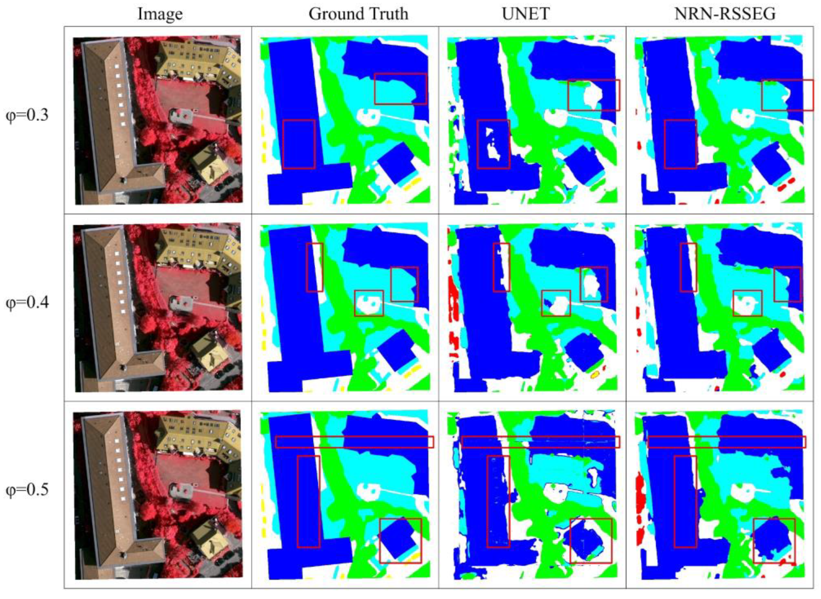
Figure 7 shows the extraction results of the two methods under different noise levels. At a noise rate of 0.3, UNET and NRN-RSSEG give similar extraction results; however, as highlighted in the red boxes, UNET misclassifies some building pixels as non-buildings and cannot distinguish low plants and trees well when the buildings are shaded. At a noise rate of 0.4, the NRN-RSSEG can identify the boundaries between each category well. When the noise rate is 0.5, the UNET predictions appear to be very unstable, there are banded misclassified samples, and even the edges of building categories appear around areas that have been categorized as plants; in contrast, the NRN-RSSEG still provides stable predictions, there are no banded or edged misclassified samples, and the categories can be well distinguished. NRN-RSSEG is therefore less affected by label noise and can better identify various land classes.

4. Discussion

NRN-RSSEG comprises three sub-modules: the UNET main network, CBAM attention module, and a modified loss function. Different sub-modules contribute to the model differently; this section focuses on exploring the magnitudes of the CBAM attention sub-module and modified loss function contributions to the model.

4.1. Contribution of CBAM to the Model

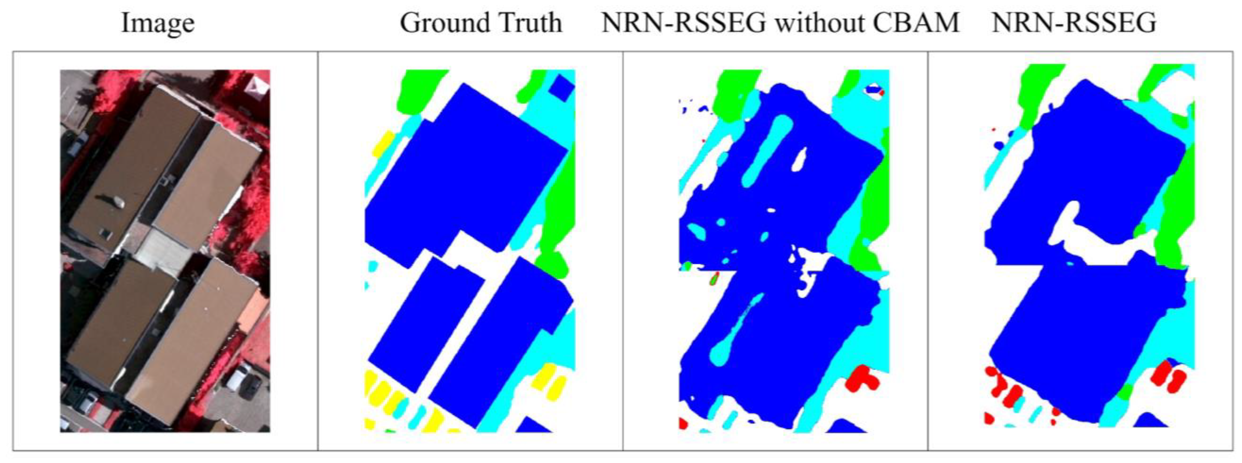
To investigate the effect of the CBAM submodule on the model predictions, we excluded it from the NRN-RSSEG, kept the other parts unchanged, and conducted experiments in a noisy environment with $\phi =0.5$ (see

Table 2. Test results of UNET and NRN-RSSEG, bold represents the high value of this assessment index at the same noise rate. (φ = noise rate).

Meath	Assessment	$\mathit{\phi }=0.5$
NRN-RSSEG without CBAM	PA	0.8027
	MPA	0.8028
	Kappa	0.7373
	Mean_F1	0.8005
	FWIoU	0.6773
NRN-RSSEG	PA	0.8058
	MPA	0.8076
	Kappa	0.7419
	Mean_F1	0.8082
	FWIoU	0.6831

). When the CBAM submodule was excluded, performance declined compared with the full NRN-RSSEG model: PA decreased by 0.31%, MAP by 0.48%, Kappa by 0.46%, Mean_F1 by 0.77%, and FWIoU by 0.58%. From the visual results (Figure 8), excluding the CBAM model submodule resulted in rougher boundaries in each category, and building interiors contained many incorrectly predicted pixels.

The experimental results confirm that the CBAM submodule can improve the performance of NRN-RSSEG. In contrast, it can also be seen that CBAM contributes less to NRN-RSSEG than does the modified loss function. The visual results indicate that the attention mechanism focuses more on the main modes and can partially eliminate the effects caused by the noisy modes. Overall, NRN-RSSEG does not show major performance degradation after eliminating the CBAM submodule; however, the visual results show that the full NRN-RSSEG model produces smoother results and lacks a large number of voids within the categories, which is more in line with human expectations.

4.2. Contribution of the Modified Loss Function to the Model

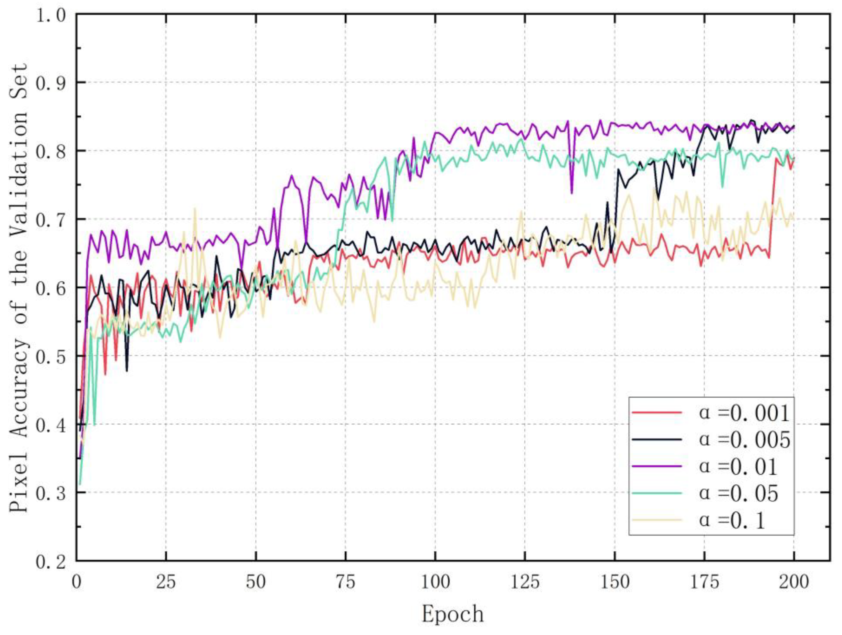
Although the CBAM submodule can make the prediction results more consistent with human expectations, the improvement in model performance is not significant. However, the improved loss function has an important impact on the model’s performance. The improved loss function includes two hyperparameters ($\alpha$ and $\beta$), whose values affect convergence and noise robustness. We conducted a series of control experiments to observe how the model converged on the validation set under different hyperparameter values: labeled noise environment with $\phi =0.5$; $\alpha$ = 0.001, 0.005, 0.01, 0.05, and 0.1, and $\beta$ was kept constant at 1.

Figure 9 shows the effects of different hyperparameters on the model in a 50% label noise environment. The pixel accuracy curves show that the convergence and noise robustness of the model are best at $\alpha =0.01$, and the accuracy curves maintain higher values in the early training period. Although the curves display small oscillations, they show a general upward trend. After the 100th epoch, the accuracy rate reached the maximum value and gradually stabilized; when $\alpha =0.05$, the accuracy rate during the early training stage was lower than that at$\alpha =0.01$, but the slope of the curve was obviously steeper and convergence was quicker; the model also gradually converged after the 100th epoch, but the overall accuracy rate was lower than that at$\alpha =0.01$. When $\alpha =0.1$, the accuracy curve showed more pronounced oscillations, and the model converged during the early training stage. At $\alpha =0.1$, the accuracy curve showed more obvious oscillations, and the model tended to converge in the early stage of training but maintained a low accuracy rate; when$\alpha =0.005$, the pixel accuracy of the model is comparable to that of $\alpha =0.01$ after 200 rounds, but the convergence rate slows down significantly, and the pixel accuracy starts to increase after the 150th round and gradually converges after 175 rounds. When $\alpha =0.001$, the pixel accuracy shows an increasing trend at the end of training, but it has not yet reached the convergence state after 200 rounds of training are completed, and the pixel accuracy is lower than that at $\alpha =0.01$ and $\alpha =0.005$. The results (Figure 9) show that the modified loss function has a greater impact than CBAM on the model results and produces robust results that can eliminate most of the effects of label noise. In addition, applying different hyperparameter values of the loss function affected the performance of the model. With a larger value of $\alpha$, the model starts to converge during the early stage of training, but it basically loses its robustness to noise. At lower values of $\alpha$, convergence begins to slow, but the robustness to noise becomes significantly stronger. Therefore, selection of appropriate hyperparameter values can simultaneously influence both the convergence and robustness of the model.

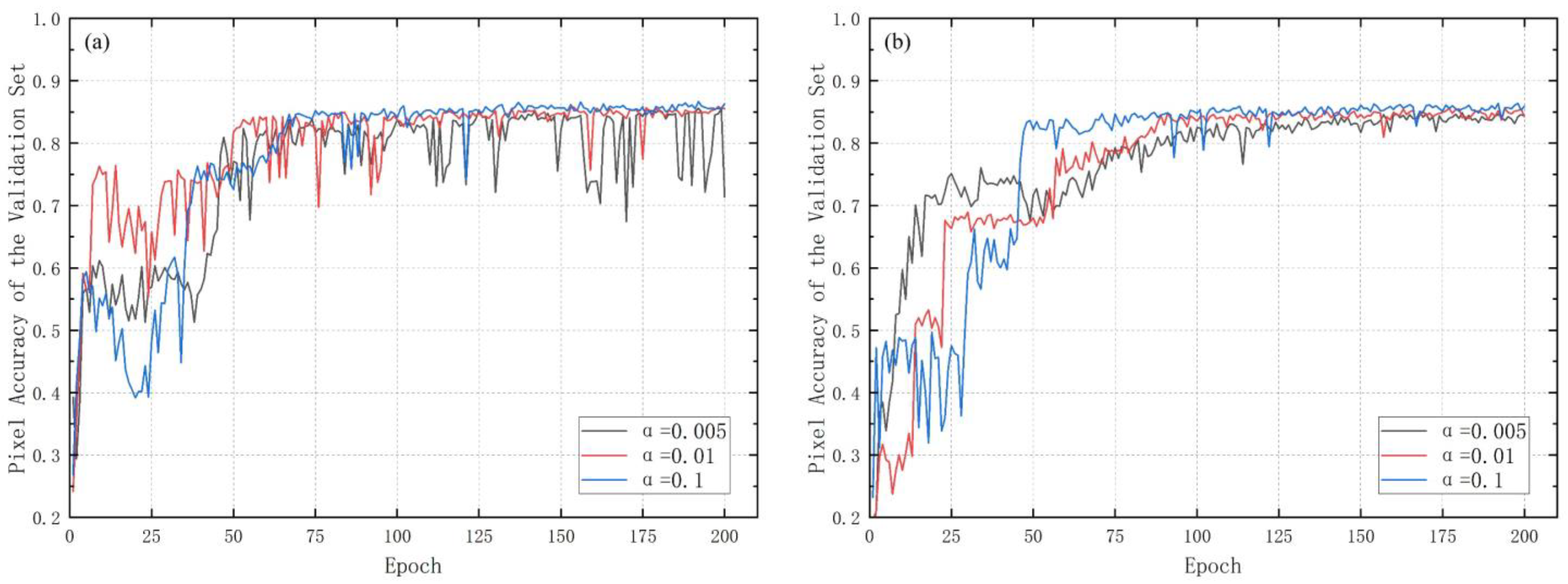
To evaluate the parameters suitable for all noise rates, we conducted experiments at 30% and 40% noise rate levels, setting α to 0.1, 0.01, and 0.005, respectively, to observe the convergence of the model. Figure 10a shows the effects of different parameter values on the pixel accuracy of the model at 30% noise rate level, and it can be seen that the model works best when for $\alpha =0.1$ and $\alpha =0.01$. When α = 0.1, the pixel accuracy curve is smoother and the model is smoother; when $\alpha =0.01$, the pixel accuracy is more oscillating in the early training and gradually smooths out in the later training period; and when α = 0.05, the pixel accuracy can also reach the maximum value, but the smoothness of the model is still not too good after 200 rounds. Figure 10b shows that under the noise rate level of 40%, the values of α are different, but they all achieve better results, and the pixel accuracy difference is quite small in the three different cases, indicating that the NRN-RSSEG performance reaches the best when the noise rate reaches a certain level, which is also consistent with the results obtained in Section 3.1. From the curve fitting, the convergence rate is slowing down as the value of α is taken to decrease. Combining Figure 9 and Figure 10, we can conclude that different hyperparameter values of the loss function have an impact on the performance of the model; when the noise rate level is low ($\phi =0.3$) or high ($\phi =0.5$), it is more sensitive to the change of the parameters, and in the case of moderate noise rate level ($\phi =0.4$), it is not obvious to the change of the parameters. In summary, in practice, we suggest setting α to 0.01. In the future, we will also set a dynamic tuning mechanism to better solve this problem.

Figure 11 shows the prediction results for different values of $\alpha$ under a 50% noise environment. The results show that $\alpha$ mainly affects the classification of low vegetation and trees; the prediction of buildings and impervious surfaces is better because of the influence of CBAM, and no voids appear. When $\alpha =0.1$, some areas of low vegetation were misclassified as trees, and building pixels were overclassified; at $\alpha =0.05$, although low vegetation and trees were distinguished, some areas of low vegetation contained voids, and they were misclassified as impervious surfaces. At $\alpha =0.01$, low vegetation and trees were well distinguished and buildings were clearly bounded although a small amount of overclassification occurred. The partitioning effect was significantly better than in the first two cases.

4.3. Comparison with Other Methods

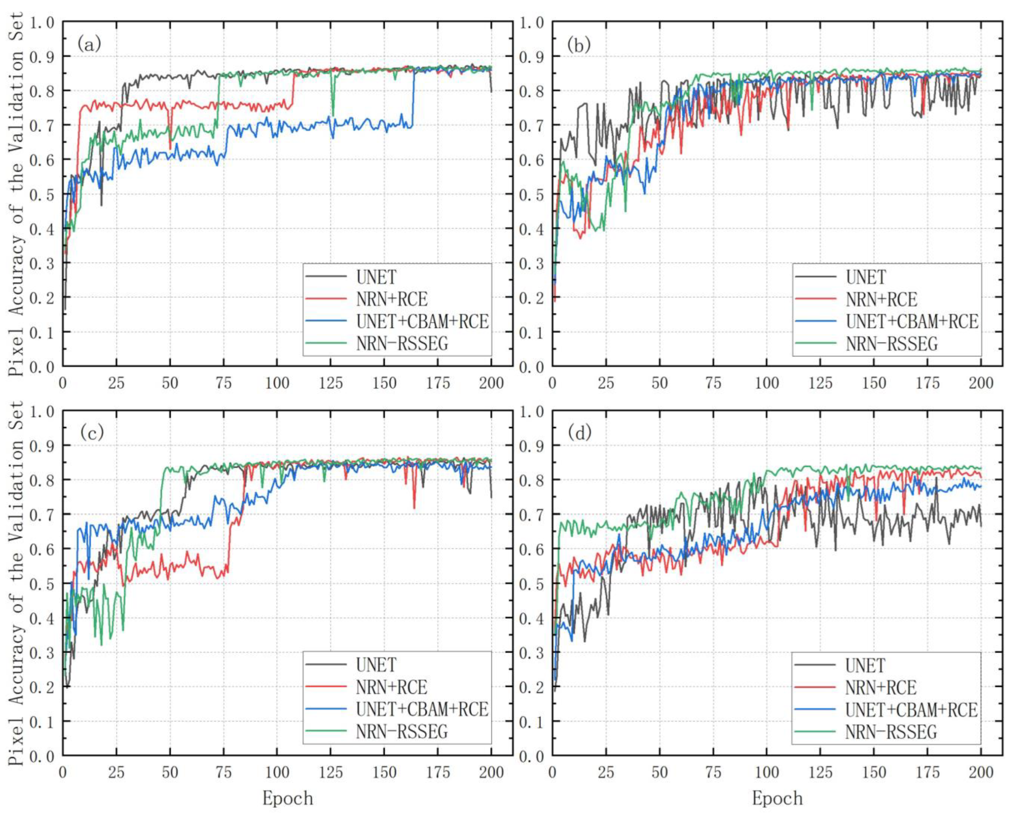
The proposed method in this paper is based on the correlation theory of UNET and RCE, therefore, we compared NRN-RSSEG with the related methods.

Table 3. Test results of different methods, bold represents the high value of this assessment index at the same noise rate. (φ = noise rate).

Meath	Assessment	$\mathit{\phi }=0$	$\mathit{\phi }=0.3$	$\mathit{\phi }=0.4$	$\mathit{\phi }=0.5$
UNET	PA	0.8288	0.8097	0.8208	0.7674
	MPA	0.8217	0.8070	0.8284	0.7790
	Kappa	0.7729	0.7455	0.7610	0.6874
	Mean_F1	0.8019	0.8056	0.7277	0.7508
	FWIoU	0.7145	0.6813	0.7007	0.6170
UNET + RCE	PA	0.8317	0.8145	0.8137	0.7498
	MPA	0.6702	0.6540	0.6610	0.7705
	Kappa	0.7761	0.7520	0.7520	0.6679
	Mean_F1	0.6684	0.6461	0.6497	0.7501
	FWIoU	0.7158	0.6873	0.6902	0.6005
UNET + CBAM + RCE	PA	0.8191	0.8219	0.7968	0.7546
	MPA	0.7890	0.8244	0.6465	0.7614
	Kappa	0.7594	0.7622	0.7285	0.6728
	Mean_F1	0.7900	0.8191	0.6323	0.7514
	FWIoU	0.6953	0.7016	0.6663	0.6055
NRN-RSSEG	PA	0.8309	0.8288	0.8287	0.8058
	MPA	0.7935	0.8312	0.8285	0.8076
	Kappa	0.7752	0.7720	0.7722	0.7419
	Mean_F1	0.7873	0.8286	0.8296	0.8082
	FWIoU	0.7157	0.7140	0.7151	0.6831

shows the evaluation results of different methods at each noise rate level, and the results show that on the clean dataset ($\mathsf{\phi }=\mathbf{0}$), there is little difference in the metrics of the four methods, and all four methods have better results on the clean dataset. When there is noise in the dataset, NRN-RSSEG outperforms the other three methods in all metrics. Figure 12 shows the pixel accuracy variation of the four methods on the validation dataset with different noise rate levels. In contrast to other methods, the training process of the model appears to be very oscillating as the noise rate increases, especially at the noise rate level of 50%.

5. Conclusions

A generalized noise-resistant network framework, NRN-RSSEG, is proposed to minimize the impact of mislabeling on remote sensing image segmentation. The framework consists of three sub-modules: the UNET main network, CBAM attention mechanism sub-module, and noise robust loss function sub-module. The UNET main network serves as the main architecture, the CBAM attention mechanism enhances the details of the network prediction results, and the noise-robust loss function suppresses the effect of label noise on image segmentation. These three submodules in combination improve the performance of the network in environments with label-noise.

From testing the proposed NRN-RSSEG model using the Vaihingen region of the ISPRS Vaihingen 2D semantic labeling dataset with three levels of simulated label noise (symmetric and asymmetric noise), we found the following:

• When the noise rate and noise level are low, UNET is less affected by label noise and exhibits a certain resistance to noise. When the label noise rate of the training set exceeded a certain threshold, the accuracy of the UNET was significantly reduced.
• For datasets with label noise, our proposed NRN-RSSEG method can maintain high accuracy and outperform the original method; this advantage becomes more obvious as label noise increases.
• The CBAM attention mechanism can improve the detailed effects of the prediction results and partially eliminate noise. The modified loss function has a greater impact on improving algorithm performance, and its hyperparameter values also affect both convergence and robustness to label noise.

In summary, a general labeled noise-robust network is proposed for the task of segmenting high-resolution remote sensing images based on deep learning, providing a CBAM attention mechanism and modified loss function that can be applied to other semantic segmentation networks. In future research, the hyperparameter selection of the loss function will also be studied in detail, and the hyperparameter taking value of the loss function will be updated dynamically for different noise environments. As the hyperparameter values of the loss function greatly influence the algorithm performance, future research may also incorporate a dynamic tuning mechanism, considering the convergence and robustness of the network.

References

1. Huang, X.; Zhang, L.P.; Gong, W. Information fusion of aerial images and LIDAR data in urban areas: Vector-stacking, re-classification and post-processing approaches. Int. J. Remote Sens. 2011, 32, 69–84. [Google Scholar] [CrossRef]
2. Lan, Z.Y.; Liu, Y. Study on Multi-Scale Window Determination for GLCM Texture Description in High-Resolution Remote Sensing Image Geo-Analysis Supported by GIS and Domain Knowledge. Isprs Int. J. Geo-Inf. 2018, 7, 175. [Google Scholar] [CrossRef] [Green Version]
3. Leichtle, T.; Geiss, C.; Lakes, T.; Taubenbock, H. Class imbalance in unsupervised change detection-A diagnostic analysis from urban remote sensing. Int. J. Appl. Earth Obs. Geoinf. 2017, 60, 83–98. [Google Scholar] [CrossRef]
4. Badrinarayanan, V.; Kendall, A.; Cipolla, R. SegNet: A Deep Convolutional Encoder-Decoder Architecture for Image Segmentation. IEEE Trans. Pattern Anal. Mach. Intell. 2017, 39, 2481–2495. [Google Scholar] [CrossRef] [PubMed]
5. Haq, M.A. CDLSTM: A Novel Model for Climate Change Forecasting. CMC-Comput. Mat. Contin. 2022, 71, 2363–2381. [Google Scholar] [CrossRef]
6. Haq, M.A. SMOTEDNN: A Novel Model for Air Pollution Forecasting and AQI Classification. CMC-Comput. Mat. Contin. 2022, 71, 1403–1425. [Google Scholar] [CrossRef]
7. Chen, Y.; Fan, R.S.; Bilal, M.; Yang, X.C.; Wang, J.X.; Li, W. Multilevel Cloud Detection for High-Resolution Remote Sensing Imagery Using Multiple Convolutional Neural Networks. Isprs Int. J. Geo-Inf. 2018, 7, 181. [Google Scholar] [CrossRef] [Green Version]
8. Kampffmeyer, M.; Salberg, A.B.; Jenssen, R. Semantic Segmentation of Small Objects and Modeling of Uncertainty in Urban Remote Sensing Images Using Deep Convolutional Neural Networks. In Proceedings of the 29th IEEE Conference on Computer Vision and Pattern Recognition (CVPR), Las Vegas, NV, USA, 26 June–1 July 2016; pp. 680–688. [Google Scholar]
9. Lin, H.N.; Shi, Z.W.; Zou, Z.X. Fully Convolutional Network with Task Partitioning for Inshore Ship Detection in Optical Remote Sensing Images. IEEE Geosci. Remote Sens. Lett. 2017, 14, 1665–1669. [Google Scholar] [CrossRef]
10. Jiao, L.C.; Liang, M.M.; Chen, H.; Yang, S.Y.; Liu, H.Y.; Cao, X.H. Deep Fully Convolutional Network-Based Spatial Distribution Prediction for Hyperspectral Image Classification. IEEE Trans. Geosci. Remote Sensing 2017, 55, 5585–5599. [Google Scholar] [CrossRef]
11. Haq, M.A. CNN Based Automated Weed Detection System Using UAV Imagery. Comput. Syst. Sci. Eng. 2022, 42, 837–849. [Google Scholar] [CrossRef]
12. Ratsch, G.; Onoda, T.; Muller, K.R. Soft margins for AdaBoost. Mach. Learn. 2001, 42, 287–320. [Google Scholar] [CrossRef]
13. Frank, J.; Rebbapragada, U.; Bialas, J.; Oommen, T.; Havens, T.C. Effect of Label Noise on the Machine-Learned Classification of Earthquake Damage. Remote Sens. 2017, 9, 803. [Google Scholar] [CrossRef] [Green Version]
14. Zhang, R.; Chen, Z.H.; Zhang, S.X.; Song, F.; Zhang, G.; Zhou, Q.C.; Lei, T. Remote Sensing Image Scene Classification with Noisy Label Distillation. Remote Sens. 2020, 12, 21. [Google Scholar] [CrossRef] [Green Version]
15. Safavian, S.R.; Landgrebe, D. A survey of decision tree classifier methodology. IEEE Trans. Syst. Man Cybern. 1991, 21, 660–674. [Google Scholar] [CrossRef] [Green Version]
16. Sukhbaatar, S.; Bruna, J.; Paluri, M.; Bourdev, L.; Fergus, R. Training convolutional networks with noisy labels. arXiv 2014, arXiv:1406.2080. [Google Scholar]
17. Hendrycks, D.; Mazeika, M.; Wilson, D.; Gimpel, K. Using Trusted Data to Train Deep Networks on Labels Corrupted by Severe Noise. In Proceedings of the 32nd Conference on Neural Information Processing Systems (NIPS), Montreal, QC, Canada, 2–8 December 2018. [Google Scholar]
18. Patrini, G.; Rozza, A.; Menon, A.K.; Nock, R.; Qu, L.Z. Making Deep Neural Networks Robust to Label Noise: A Loss Correction Approach. In Proceedings of the 30th IEEE/CVF Conference on Computer Vision and Pattern Recognition (CVPR), Honolulu, HI, USA, 21–26 July 2017; pp. 2233–2241. [Google Scholar]
19. Goldberger, J.; Ben-Reuven, E. Training Deep Neural-Networks Using a Noise Adaptation Layer. In Proceedings of the International Conference on Learning Representations, Toulon, France, 4 November 2016. [Google Scholar]
20. Huang, J.C.; Qu, L.; Jia, R.F.; Zhao, B.Q. O2U-Net: A Simple Noisy Label Detection Approach for Deep Neural Networks. In Proceedings of the IEEE/CVF International Conference on Computer Vision (ICCV), Seoul, Republic of Korea, 27 October–2 November 2019; pp. 3325–3333. [Google Scholar]
21. Brooks, J.P. Support Vector Machines with the Ramp Loss and the Hard Margin Loss. Oper. Res. 2011, 59, 467–479. [Google Scholar] [CrossRef] [Green Version]
22. van Rooyen, B.; Menon, A.K.; Williamson, R.C. Learning with Symmetric Label Noise: The Importance of Being Unhinged. In Proceedings of the 29th Annual Conference on Neural Information Processing Systems (NIPS), Montreal, QC, Canada, 7–12 December 2015. [Google Scholar]
23. Ghosh, A.; Kumar, H.; Sastry, P.S. Robust Loss Functions under Label Noise for Deep Neural Networks. In Proceedings of the 31st AAAI Conference on Artificial Intelligence, San Francisco, CA, USA, 4–9 February 2017; pp. 1919–1925. [Google Scholar]
24. Zhang, Z.; Jiang, G.; Wang, W. Label noise filtering method based on local probability sampling. J. Comput. Appl. 2021, 41, 67–73. [Google Scholar]
25. Northcutt, C.G.; Jiang, L.; Chuang, I.L. Confident Learning: Estimating Uncertainty in Dataset Labels. J. Artif. Intell. Res. 2021, 70, 1373–1411. [Google Scholar] [CrossRef]
26. Jindal, I.; Nokleby, M.; Chen, X.W. Learning Deep Networks from Noisy Labels with Dropout Regularization. In Proceedings of the 16th IEEE International Conference on Data Mining (ICDM), Barcelona, Spain, 12–15 December 2016; pp. 967–972. [Google Scholar]
27. Sun, Y.; Tian, Y.; Xu, Y.P.; Li, J.X. Limited Gradient Descent: Learning with Noisy Labels. IEEE Access 2019, 7, 168296–168306. [Google Scholar] [CrossRef]
28. Nguyen, A.; Yosinski, J.; Clune, J. Deep Neural Networks are Easily Fooled: High Confidence Predictions for Unrecognizable Images. In Proceedings of the IEEE Conference on Computer Vision and Pattern Recognition (CVPR), Boston, MA, USA, 7–12 June 2015; pp. 427–436. [Google Scholar]
29. Jian, L.; Gao, F.H.; Ren, P.; Song, Y.Q.; Luo, S.H. A Noise-Resilient Online Learning Algorithm for Scene Classification. Remote Sens. 2018, 10, 1836. [Google Scholar] [CrossRef] [Green Version]
30. Ren, M.Y.; Zeng, W.Y.; Yang, B.; Urtasun, R. Learning to Reweight Examples for Robust Deep Learning. In Proceedings of the 35th International Conference on Machine Learning (ICML), Stockholm, Sweden, 10–15 July 2018. [Google Scholar]
31. Pham, H.; Dai, Z.H.; Xie, Q.Z.; Le, Q.V.; Ieee Comp, S.O.C. Meta Pseudo Labels. In Proceedings of the IEEE/CVF Conference on Computer Vision and Pattern Recognition (CVPR), Electr Network, Nashville, TN, USA, 19–25 June 2021; pp. 11552–11563. [Google Scholar]
32. Ghosh, A.; Manwani, N.; Sastry, P.S. Making risk minimization tolerant to label noise. Neurocomputing 2015, 160, 93–107. [Google Scholar] [CrossRef] [Green Version]
33. Feng, L.; Shu, S.L.; Lin, Z.Y.; Lv, F.M.; Li, L.; An, B. Can Cross Entropy Loss Be Robust to Label Noise? In Proceedings of the 29th International Joint Conference on Artificial Intelligence, Electr Network, Yokohama, Japan, 7–15 January 2021; pp. 2206–2212. [Google Scholar]
34. Saberi, N.; Scott, K.A.; Duguay, C. Incorporating Aleatoric Uncertainties in Lake Ice Mapping Using RADARSAT-2 SAR Images and CNNs. Remote Sens. 2022, 14, 644. [Google Scholar] [CrossRef]
35. Cao, Y.C.; Wu, Y.; Zhang, P.; Liang, W.K.; Li, M. Pixel-Wise PolSAR Image Classification via a Novel Complex-Valued Deep Fully Convolutional Network. Remote Sens. 2019, 11, 2653. [Google Scholar] [CrossRef] [Green Version]
36. Rottensteiner, F.; Sohn, G.; Gerke, M.; Wegner, J.D. ISPRS semantic labeling contest. ISPRS Leopoldshöhe Ger. 2014, 1, 4. [Google Scholar]
37. Vaswani, A.; Shazeer, N.; Parmar, N.; Uszkoreit, J.; Jones, L.; Gomez, A.N.; Kaiser, L.; Polosukhin, I. Attention Is All You Need. In Proceedings of the 31st Annual Conference on Neural Information Processing Systems (NIPS), Long Beach, CA, USA, 4–9 December 2017. [Google Scholar]
38. Ronneberger, O.; Fischer, P.; Brox, T. U-Net: Convolutional Networks for Biomedical Image Segmentation. In Proceedings of the 18th International Conference on Medical Image Computing and Computer-Assisted Intervention (MICCAI), Munich, Germany, 5–9 October 2015; pp. 234–241. [Google Scholar]
39. Woo, S.H.; Park, J.; Lee, J.Y.; Kweon, I.S. CBAM: Convolutional Block Attention Module. In Proceedings of the 15th European Conference on Computer Vision (ECCV), Munich, Germany, 8–14 September 2018; pp. 3–19. [Google Scholar]
40. Wang, Y.S.; Ma, X.J.; Chen, Z.Y.; Luo, Y.; Yi, J.F.; Bailey, J. Symmetric Cross Entropy for Robust Learning with Noisy Labels. In Proceedings of the IEEE/CVF International Conference on Computer Vision (ICCV), Seoul, Republic of Korea, 27 October–2 November 2019; pp. 322–330. [Google Scholar]
41. Wang, Z.; Zhou, Y.; Wang, S.; Wang, F.; Xu, Z. House building extraction from high-resolution remote sensing images based on IEU-Net. J. Remote Sens. 2021, 25, 2245–2254. [Google Scholar]
42. Krizhevsky, A.; Sutskever, I.; Hinton, G.E. ImageNet Classification with Deep Convolutional Neural Networks. Commun. ACM 2017, 60, 84–90. [Google Scholar] [CrossRef] [Green Version]
Figure 1. Example of ISPRS Vaihingen 2D Semantic Labeling dataset (left image is remote sensing image data, right image is label data).
Remotesensing 15 00108 g001
Figure 2. Examples of symmetric and asymmetric label noise. Different grayscale values represent different flipping probabilities: (a) is symmetric label noise: real labels are flipped to other labels with equal probability; (b) is asymmetric label noise: real labels are flipped to other labels based on fixed rules.
Remotesensing 15 00108 g002
Figure 3. Improved UNET model structure.
Remotesensing 15 00108 g003
Figure 4. Schematic diagram of CBAM module structure: (a) is the general schematic of the CBAM module, (b) shows the Channel Attention Module, and (c) is the Spatial Attention Module.
Remotesensing 15 00108 g004
Figure 5. Schematic diagram of sliding window prediction.
Remotesensing 15 00108 g005
Figure 6. Pixel accuracy curves for the two models using the validation dataset with different noise rates. (a) clean data set, (b) with 30% noise rate, (c) 40% noise rate, (d) 50% noise rate.
Remotesensing 15 00108 g006
Figure 7. UNET and NRN-RSSEG predictions at different noise rates (0.3, 0.4 and 0.5).
Remotesensing 15 00108 g007
Figure 8. Predictions of full NRN-RSSEG model and after excluding CBAM (50% noise rate).
Remotesensing 15 00108 g008
Figure 9. Effect of different α on NRN-RSSEG in 50% label noise environment.
Remotesensing 15 00108 g009
Figure 10. Effect of different α on NRN-RSSEG in 30% and 40% label noise environments. (a) with 30% noise rate, (b) 40% noise rate.
Remotesensing 15 00108 g010
Figure 11. Prediction results for different α in 50% label noise environment.
Remotesensing 15 00108 g011
Figure 12. Pixel accuracy curves for four models using validation datasets with different noise rates. (a) clean dataset, (b) with 30% noise rate, (c) 40% noise rate, (d) 50% noise rate.
Remotesensing 15 00108 g012