Fast Displacement Estimation of Multiple Close Targets with MIMO Radar and MUSICAPES Method

Abstract

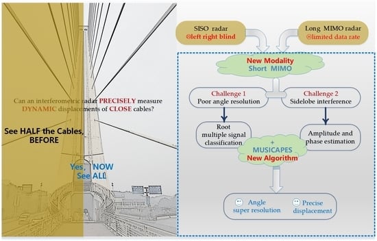
Interferometric radar is a hot research topic in manmade target displacement measuring applications, as it features high precision, a large operation range, and a remote multiple point measuring ability. Most one-dimensional interferometric radars use single-input single-output (SISO) radar architecture to achieve a high repetition measuring rate of more than 200 Hz; however, it cannot resolve multiple targets with the same radial range but different azimuth angles. This paper presents a multiple-input multiple-output (MIMO) radar that adopts a limited number of antennas (usually tens) to simultaneously improve azimuth resolution and achieve a high repetition measuring rate. A MUSICAPES algorithm is proposed, which is cascades the multiple signal classification (MUSIC) algorithm and the amplitude and phase estimation (APES) filter. The MUSIC algorithm is used to further improve the angular resolution of the small array. The APES is used to precisely recover the phases of the multiple close targets by suppressing their mutual interferences. Simulations and experiments with a millimeter-wave radar validate the performance of the proposed method.

1. Introduction

Many manmade targets, such as bridges, tunnels, towers, tall buildings, etc., deform slightly under external forces. These external forces are wind, traffic, hydraulic, temperature stress, or a combination of them. The deformation may cause irreversible structural damage if it exceeds the maximum deformation threshold; therefore, it is of great significance to precisely monitor the tiny deformations of these targets. At present, deformation can be measured by contact or non-contact deformation measuring sensors. Conventional contact measurement sensors include displacement gauge, tension gauge, accelerometer, vibration pickup, strain gauge, inclinometer, level gauge, and Beidou/GPS displacement gauge. Non-contact sensors include total station, laser interferometry, high-definition video, interferometric radar, etc. According to the working mode, the most widely used deformation measuring sensors belong to the single-point measurement system; however, they suffer several technical limitations. Interferometric radars are popular for monitoring bridges, towers, slopes, mine pits, dams, and other civil infrastructures.

Interferometric radars receive the echo of an object’s backscattering by transmitting microwave radio waves and measuring the displacement of the object by time difference interferometry. They feature high precision, long working range, operational convenience, remote multiple point measuring ability, and good environmental adaptability [1]. They can be further divided into one-dimensional interferometric radars and two-dimensional interferometric radars. The former kind of radars is applied to measure bridges, tall buildings, and towers, which requires a higher repetition measurement rate [2,3], whereas the latter kind is applied to measure slopes and dams, which features a lower repetition rate but a large coverage requirement [4]. Interferometric radars can be extended to different platforms, such as satellites, airplanes, ships, and rails [5]. These radars would also work at different frequency bands, from the X band up to the W band [6].

One-dimensional interferometric radars generally adopt the single-input signal-output (SISO) radar architecture. The radar can only measure the deformations of objects with different radial distances. It would hinder the radar’s application in the case of there being two objects with the same radial distance but different azimuth angles. Most amendments to these radars are to solve displacements with multiple directions [7]. If a one-dimensional interferometric radar adopts multiple-input multiple-output (MIMO) radar architecture, its multiple targets resolving capability can be improved. Traditional MIMO interferometric radars are usually proposed to reduce the data acquisition time of rail-mounted two-dimensional interferometric radars [8,9]. Some improvements to MIMO interferometric radars would involve forming 3-D images and retrieving 3-D displacements [10,11]. Few MIMO radars are capable of even measuring dynamic displacements [12], and many of them find it hard to achieve a high repetition rate similar to that of a one-dimensional radar.

Multiple target imaging algorithms for MIMO interferometric radar include the back projection (BP) algorithm [8], the range migration algorithm, and the far-field pseudo-polar format algorithm (FPFA) [13]. All these algorithms are suitable when the equivalent elements of a MIMO array are large; however, a large repetition rate requires a smaller MIMO array. The imaging algorithm should adapt to the small array while still having a fine multiple-target resolving ability. As the range migration of a target is not prominent for the small array, fast Fourier transformation (FFT) can be used to resolve multiple targets. Although improved methods such as ZOOM-FFT(ZFFT), FFT-FS, and chirp z-transform (CZT) [14], can be used to improve the computation resolution. These FFT-based methods still suffer from a limited angle resolution that is inversely proportional to the array length. Direction of arrival (DOA) estimation methods can achieve a better performance when scatters are independent. These methods include Capon beamforming [15], the amplitude and phase estimation (APES) [16,17], the multiple signal classification (MUSIC) [18,19], and so on. The phases of multiple targets would suffer mutual interferences if they were close. It would cause additional requirements for the DOA methods. None of these methods can achieve azimuth super-resolution and precise phase estimation at the same time.

In this paper, a short MIMO interferometric radar is designed to extract multiple close targets with a high repetition rate. A MUSICAPES algorithm is proposed to resolve multiple targets beyond the angle resolution and suppress the mutual interferences of their side lobes. The algorithm is performed by cascading the root-MUSIC algorithm and an APES filter. The deformations of multiple targets with the same radial distance but different azimuth angles are finally accurately estimated with time differential interferometry. The main contributions of this paper are summarized as follows.

• A MIMO interferometric radar is proposed for a precise, high repetition rate, non-contact, multi-point simultaneous displacement measurement. It has the advantages of both one-dimensional and two-dimensional deformation measuring radars. It can measure multiple close targets such as complex bridges, towers, and buildings, which traditional one-dimensional radars fail to do.
• A MUSICAPES method is proposed to resolve multiple azimuth close targets and precisely extract their displacements. The method first adopts the root-MUSIC algorithm to estimate the azimuth angle of each target. Then, the APES algorithm is used to precisely recover the phases of the targets using the azimuth angles estimated in the former step. The method can improve the displacement measuring precision significantly.
• A millimeter-wave MIMO interferometric radar is designed for multiple target displacement measuring. The radar is composed of a commercial off-the-shelf (COTS) radar front end, an analog to digital (AD) card, and a laptop computer. Experiment results show that the radar can resolve multiple targets beyond the angular resolution of the MIMO array and can precisely measure their displacements at a repetition rate of more than 100 Hz.

Notation: We denote vectors and matrices by boldface letters. See

Table 1. Meanings of main abbreviations, acronyms and symbols.

Index	Term	Meaning
1	SISO	single-input signal-output
2	MIMO	multiple-input multiple-output
3	MUSIC	multiple signal classification
4	APES	amplitude and phase estimation
5	CZT	chirp z-transform
6	DOA	direction of arrival
7	MMW	millimeter-wave
8	COTS	commercial off-the-shelf
9	$R_1$	input covariance matrix for MUSIC
10	$R_2$	input covariance matrix for APES
11	$U_S$	signal space by eigen decomposition
12	$U_N$	noise space by eigen decomposition
13	$\widehat{Q}$	noise covariance matrix for APES
14	$h$	optimal complex filter coefficients of APES

for the main acronyms and symbols and their meanings.

The rest of this paper is organized as follows. Section 2 briefly describes the architecture of the MIMO interferometric radar and the principles of multiple target discrimination. A MUSICAPES method is proposed in Section 3, to precisely extract the displacements of multiple close targets. Simulations and two-target displacement measuring experiments with an MMW MIMO radar are presented in Section 4. Finally, conclusions are drawn in Section 5.

2. MIMO Interferometric Radar and Multiple Target Discrimination

Conventional one-dimensional interferometric radars adopt one transmitting antenna and one receiving antenna. The azimuth resolution is restricted to the beamwidth of the two antennas. Generally speaking, the radar cannot resolve two targets with the same radial range but different cross-range positions, as target A and target B in Figure 1, for example. The radar can only resolve targets with different radial ranges, as target A and target C in Figure 1, for example.

Azimuth or angle discrimination can be improved by using a SAR or DOA algorithm in traditional radars. Two-dimensional interferometric radars adopt the SAR system and the persistent scatter (PS) algorithm to estimate slow displacement. We use the DOA method to estimate fast displacement. The radar architecture, the principles of range discrimination, and azimuth discrimination are described in this section in detail.

2.1. Basic Architecture of an Interferometric MIMO Radar

To achieve a high repetition measuring rate, all the transmitting and receiving channels of a MIMO radar should work simultaneously. The radar should adopt an orthogonal waveform, multiple transmitters, and multiple receivers to achieve the best performance; however, the overall cost of the radar would be unaffordable in most civil applications. Moreover, we will use the MIMO radar that works in time-division mode.

The MIMO interferometric radar is composed of M transmitting antennas and N receiving antennas, as shown in Figure 2. The space between two receiving antennas is half the wavelength. The interval between two transmitting antennas is N times the half wavelength. As a result, an equivalent transceiving antenna array is formed. The interval between two equivalent antennas is a quarter of the wavelength. In a far-field assumption, the equivalent transceiving antenna TR_ij is in the middle of the transmitting antenna T_i and the receiving antenna R_j.

$$x_{T{R}_{ij}}=\left(x_{T_i}+x_{R_j}\right)/2\hspace{1em}{y}_{T{R}_{ij}}=\left(y_{T_i}+y_{R_j}\right)/2$$

(1)

where $x_{T_i}, x_{R_j}, x_{T{R}_{ij}}$ are positions in the x coordinate of the ith transmitting antenna, the jth receiving antenna, and the equivalent transceiving antenna, respectively. $y_{T_i}, y_{R_j}, y_{T{R}_{ij}}$ are positions in the y coordinate of the ith transmitting antenna, the jth receiving antenna, and the equivalent transceiving antenna, respectively.

The transmitting antenna is connected to an RF switch whose input port is connected to the transmitter. Each receiving antenna is fed to a receiver that performs bandpass filter, low noise amplification, and dechirp demodulation. Then, the outputted echo is fed to an analog-to-digital converter whose output is sent to a laptop computer via Ethernet. A laptop computer controls the radar front end through a serial port, to configure the working frequency range, the sweep duration of a linear frequency modulation (LFM) signal, the pulse repetition frequency, the AD sampling frequency, and the sampling length. The sampled radar echo is streamed out through an LVDS bus to a data acquisition board which formats the echo into standard UDP socket packages. The packages are finally sent to the laptop computer via Ethernet.

2.2. Multiple Target Discriminator from the Range Direction

To distinguish nearby targets, the interferometric MIMO radar has to emit wideband signals. The LFM signal is one of the most widely used waveforms. The frequency of an LFM signal changes linearly with time. It can be formulated as

$$s_t\left(t\right)=A\times \mathrm{rect}\left(\frac{t}{T}\right)\exp \left[j\pi \left(2f_{0}t+K_f{t}^2\right)\right]\hspace{1em}0<t<T$$

(2)

where $f_0$ is the start frequency, $T$ is the sweep period, and $K_f$ is the chirp rate. $A$ is the amplitude, and it is often omitted for simplicity. The function rect is defined as $\mathrm{rect}(x)=\{\begin{array}{l}1,\hspace{1em}\left|x\right|\le 1\\ 0,\hspace{1em}\left|x\right|>1\end{array}$. The received signal of a point target is an attenuated -and time-delayed replica of the transmitting signal. After a dechirp demodulation operation, the received intermediate-frequency signal can be written as

$$s_{\mathrm{IF}}^{(T_i,R_j)}\left(t\right)=\exp \left(j2\pi f_0\tau \right)\exp \left(j2\pi K_f\tau t\right)\exp \left(-j\pi K_f{\tau }^2\right)$$

(3)

where the first exponential component indicates the phase delay; the second component is a linear phase term and indicates the range of the target; the last component is the quadratic phase error of the dechirp operation. $\tau =\left(r_{k,T_i}+r_{k,R_j}\right)/c$ is the round trip travelling delay of the electromagnetic wave. $r_{k,T_i}, r_{k,R_j}$ are the distances from the kth target to the transmitting antenna T_i, and the receiving antenna R_j, respectively. c is the electromagnetic wave velocity.

$$\begin{array}{l}{r}_{k,T_i}=\sqrt{{\left(x_k-x_{T_i}\right)}^2+{\left(y_k-y_{T_i}\right)}^2}\hspace{1em}{T}_i=1,\cdots M\\ r_{k,R_j}=\sqrt{{\left(x_k-x_{R_j}\right)}^2+{\left(y_k-y_{R_j}\right)}^2}\hspace{1em}{R}_j=1,\cdots N\end{array}$$

(4)

A one-dimensional radar image is obtained by the FFT operation and is expressed as

$$S_{\mathrm{RC}}^{(T_i,R_j)}(n)\approx N_T\exp \left[j2\pi \left(f_0\tau -\frac{1}{2}{K}_f{\tau }^2\right)\right]\exp \left[j\pi \left(\frac{K_f\tau }{f_s}-\frac{n}{N_{\mathrm{FFT}}}\right)(N_{\mathrm{FFT}}-1)\right]\sin \mathrm{c}\left[\left(\frac{K_f\tau }{f_s}-\frac{n}{N_{\mathrm{FFT}}}\right)N_{\mathrm{FFT}}\right]$$

(5)

where $N_{\mathrm{FFT}}$ is the length of the FFT operation. $f_s$ is the sampling frequency of the AD card. The one-dimensional radar image of the target is a peak whose index is $n_{\mathrm{peak}}=\mathrm{round}\left(N_{\mathrm{FFT}}{K}_f\tau /f_s\right)$. The complex radar response of the target is denoted as $\alpha (n_{\mathrm{peak}})=\exp \left[j\pi \left(2f_0\tau -K_f{\tau }^2\right)\right]$. As the second term is far less than the first one, we can obtain the phase of the target as

$$\phi (T_i,R_j,n_{\mathrm{peak}})=2\pi f_0\tau$$

(6)

The range resolution of the radar is proportional to the time duration T-τ. As $T$ is much larger than $\tau$, so is the resolution ${\rho }_r=0.886c/(K_{f}T)$. The coefficient 0.886 is a correction factor that makes the range resolution accurate [20]. If we want to discriminate between target A and target C in Figure 1, ${\rho }_r$ should be smaller than $\sqrt{{\left(x_1-x_3\right)}^2+{\left(y_1-y_3\right)}^2}$.

2.3. Multiple Target Discriminator from the Cross Range Direction

Each combination of T_i and R_j can output a one-dimensional radar image. The responses of a target in all the images have similar ranges and amplitudes, but they are different in phases. Figure 3 shows the geometry of DOA estimation with the equivalent MIMO array. If the DOA angle of the target is θ, then the phase difference between two adjacent antennas is $\pi \sin \theta$.

At the discrete time tick $t_s$, a target response vector can be constructed by using the target’s peaks in all the $M\times N$ one-dimensional images.

$$S(t_s,n_{peak})={\left[s_{\mathrm{RC}}^{(1,1)}(n_{peak}),s_{\mathrm{RC}}^{(1,2)}(n_{peak}),\cdots ,s_{\mathrm{RC}}^{(1,N)}(n_{peak}),\cdots ,s_{\mathrm{RC}}^{(M,N)}(n_{peak})\right]}^T$$

(7)

The DOA angle θ can be estimated by the traditional FFT operation. An angle response image of the target is famulated as

$$s_{SP}(t_s,k)=A{e}^{i{\overline{\varphi }}_0}\frac{\sin \left[MN\pi \left(k/(MN)+\sin \theta /2\right)\right]}{\sin \left[\pi \left(k/(MN)+\sin \theta /2\right)\right]}$$

(8)

The DOA angle θ coincides with the peak of the angle image. We can find that the angular resolution ${\rho }_{\theta }$ of an $M\times N$ array is

$${\rho }_{\theta }=\mathrm{asin}\left(\frac{2\times 0.886}{\mathrm{MN}}\right)$$

(9)

where the coefficient 0.886 is a correction factor to make the angular resolution accurate. If we want to discriminate between target A and target B in Figure 1, the resolution ${\rho }_{\theta }$ should be smaller than $\mathrm{asin}\left[\left|x_1-x_3\right|/\sqrt{{\left(x_1-x_3\right)}^2+{\left(y_1-y_3\right)}^2}\right]$.

3. MUSICAPES for Multiple Close Targets Deformation Estimation

Since the array length of the interferometric MIMO radar is small enough to maintain a high repetition measuring rate, and if the traditional MIMO radar processing method is used to estimate the displacements of multiple targets, it has to face two challenges. One challenge is that the angular resolution of the array is limited. The other one is that the large side lobes of the array would cause prominent phase errors. As a result, the radar would find it difficult to precisely estimate the displacements of multiple close targets. A MUSICAPES is proposed to solve the two problems. Firstly, the method adopts the root-MUSIC algorithm to improve the angular resolution of the short MIMO radar. Then, it employs the APES filter to suppress the interferences of other targets and precisely estimate the complex coefficients, using the DOA angle obtained by the root-MUSIC algorithm. Finally, the displacement is calculated by the traditional time differential operation.

3.1. Multiple Targets Extraction Based on MUSIC

There are many advanced array processing algorithms for DOA estimation, such as Capon beamforming, MUSIC, ESPRIT, IAA [21], and so on. We will adopt the widely used MUSIC algorithm to estimate DOA angles, as the algorithm is famous for its super-resolution performance. The MUSIC algorithm can be incorporated with phase interferometry to improve the performance of DOA estimation [22].

The input to the MUSIC algorithm is one snapshot of the MIMO array, as shown in (7). The length of the observation is $(M\times N)$. Firstly, we have to estimate the covariance of the observation. An estimation of the covariance matrix is usually obtained by (time) averaging several independent snapshots; however, there is only one snapshot, so we have to divide the long snapshot vector into several overlapped shorter subvectors. Supposing the length of the subvectors is ${\mathrm{M}}_{\mathrm{music}}$ (${\mathrm{M}}_{\mathrm{music}}\le (MN)/2$ generally), then an estimation of the input covariance matrix can be formulated as follows.

$$R_1={\displaystyle {\sum }_{i=0}^{N_{\overline{TR}}-{\mathrm{M}}_{\mathrm{music}}}{y}_1(i)\times }{\left(y_1(i)\right)}^H$$

(10)

where ${()}^{\mathrm{H}}$ is the conjunction transpose operator. The subvector is $y_1(i)={[s\left(t_s,n_{peak},i\right),s\left(t_s,n_{peak},i+1\right),\cdots s\left(t_s,n_{peak},i+{\mathrm{M}}_{\mathrm{music}}-1\right)]}^T$. Then, the eigendecomposition is performed, which can be expressed as

$$R_1=U\mathrm{\Lambda }{U}^H=U_S{\mathrm{\Lambda }}_S{U}_S^H+U_N{\mathrm{\Lambda }}_N{U}_N^H$$

(11)

There are ${\mathrm{M}}_{\mathrm{music}}$ eigenvalues, among which bigger ones are indicators of targets, and smaller ones are indicators of noise. Supposing there are P bigger eigenvalues, the corresponding eigenvectors in $U$ span a signal space which is denoted as $U_S$. The dimensions of $U_S$ are ${\mathrm{M}}_{\mathrm{music}}\times \mathrm{P}$. The remaining eigenvectors in $U$ span the noise space which is expressed as $U_N$. The dimensions of $U_N$ are ${\mathrm{M}}_{\mathrm{music}}\times \left({\mathrm{M}}_{\mathrm{music}}-\mathrm{P}\right)$.

The traditional MUSIC algorithm estimates DOA angles by finding peaks of the pseudospectrum. The pseudospectrum estimate is defined as

$$P_{MUSIC}(\theta )=\frac{1}{{\left[a_1(\theta )\right]}^H{U}_N{U}_N^H{a}_1(\theta )}$$

(12)

where $a_1(\theta )={[1,e^{-j4\pi \sin \theta d/\lambda },\cdots ,e^{-j4\pi \sin \theta {\mathrm{M}}_{\mathrm{music}}d/\lambda }]}^T$ is the steering vector of DOA angle θ. It is time-consuming to calculate the pseudo spectrum if the number of tested angles is large. The root-MUSIC can reduce the computation load. MUSIC and root-MUSIC have the same asymptotic performances, but the latter one has better performance in small sample situations [23]. The DOA angle can be estimated by solving the equation below [24].

$$z^{M_{APES}-1}{p}^T(z^{-1})U_N{U}_N^{H}p(z)=0$$

(13)

The steering vector $a_1(\theta )$ is replaced by vector $p(z)={[1,z,\cdots z^{{\mathrm{M}}_{\mathrm{music}}-1}]}^T$. Where $z=e^{-j4\pi \sin \theta d/\lambda }$. There are ${2\mathrm{M}}_{\mathrm{music}}$ solutions for Equation (13). They are symmetrical with respect to the unit circle. We choose the P solutions that are most close to the unit circle. Suppose the solutions are ${\theta }_1,{\theta }_2,\cdots {\theta }_{\mathrm{P}}$.

3.2. Deformation Estimation Based on APES

APES is a maximum likelihood estimation of the complex sinusoidal signal, which is proposed by Li and Stoica. It can obtain more precise phase and amplitude estimations than those of the Capon filter [16]. For a target angle ${\theta }_k$ estimated by the root-MUSIC, a steering vector is formed as $a_{{\mathrm{M}}_{\mathrm{APES}}}({\theta }_k)={[1,e^{-j4\pi \sin {\theta }_{k}d/\lambda },\cdots e^{-j(M_{\mathrm{APES}}-1)4\pi \sin {\theta }_{k}d/\lambda }]}^T$. ${\mathrm{M}}_{\mathrm{APES}}$ is the length of the APES filter. The complex coefficients are obtained by solving the following problem.

$$\underset{h,\alpha }{\min }\frac{1}{L}{\displaystyle {\sum }_{l=0}^{L-1}{\left|h^H{y}_2(l)-\alpha ({\theta }_k)e^{j4\pi l\sin {\theta }_{k}d/\lambda }\right|}^2},\begin{array}{cc}Subject& to\end{array}:h^H{a}_{{\mathrm{M}}_{\mathrm{APES}}}({\theta }_k)=1$$

(14)

where $y_2(l)={[s\left(t_s,n_{peak},l\right),s\left(t_s,n_{peak},l+1\right),\cdots s\left(t_s,n_{peak},l+{\mathrm{M}}_{\mathrm{APES}}-1\right)]}^T$; $h$ is a filter weighting coefficient of length ${\mathrm{M}}_{\mathrm{APES}}$. $L=\mathrm{M}\times {\mathrm{N}-\mathrm{M}}_{\mathrm{APES}}+1$. By some manipulations, the minimization problem is converted into a linear minimization, as shown below

$$\underset{h}{\min }{h}^H\widehat{Q}h\hspace{1em}subject to: h^H{a}_{{\mathrm{M}}_{\mathrm{APES}}}(\omega )=1$$

(15)

where $\widehat{Q}=R_2-g({\theta }_k)g^H({\theta }_k)$ and $R_2=\frac{1}{L}{\displaystyle {\sum }_{l=0}^{L-1}{y}_2(l)}{\left(y_2(l)\right)}^H$. $g({\theta }_k)$ is the Fourier transformation of $y_2(l)$. The optimal complex coefficients can be obtained by a Lagrange multiplication [16].

$$h=\frac{{\widehat{Q}}^{-1}{a}_{{\mathrm{M}}_{\mathrm{APES}}}({\theta }_k)}{a_{{\mathrm{M}}_{\mathrm{APES}}}^{\mathrm{H}}({\theta }_k){\widehat{Q}}^{-1}{a}_{{\mathrm{M}}_{\mathrm{APES}}}({\theta }_k)}$$

(16)

$$\widehat{\alpha }({\theta }_k)=a_{{\mathrm{M}}_{\mathrm{APES}}}^{\mathrm{H}}({\theta }_k)h$$

(17)

The matrix inversion operation in APES is computation intensive. It can be reduced by using the matrix inversion lemma. Then a new formulation of ${\widehat{Q}}^{-1}$ is

$${\widehat{Q}}^{-1}=R_2^{-1}-\frac{R_2^{-1}g({\theta }_k)g^H({\theta }_k)R_2^{-1}}{g^H({\theta }_k)R_2^{-1}g({\theta }_k)-1}$$

(18)

The computation efficiency is improved as direct matrix inversions are prevented. By substituting Equation (18) into Equation (17), a new expression of the coefficients is obtained as follows

$$\widehat{\alpha }({\theta }_k)=\frac{a_{{\mathrm{M}}_{\mathrm{APES}}}^{\mathrm{H}}({\theta }_k)R_2^{-1}g({\theta }_k)}{\left(g^H({\theta }_k)R_2^{-1}g({\theta }_k)-1\right)a_{{\mathrm{M}}_{\mathrm{APES}}}^{\mathrm{H}}({\theta }_k)R_2^{-1}{a}_{{\mathrm{M}}_{\mathrm{APES}}}({\theta }_k)-{\left|a_{{\mathrm{M}}_{\mathrm{APES}}}^{\mathrm{H}}({\theta }_k)R_2^{-1}g({\theta }_k)\right|}^2}$$

(19)

The phase difference between two coefficients estimated at $t_s$ and $t_{s+1}$ can be written as

$$\Delta \varphi (t_s,{\theta }_k)=phase(\widehat{\alpha }(t_{s+1},{\theta }_k)\times {\widehat{\alpha }}^{\ast }(t_s,{\theta }_k))$$

(20)

where $phase()$ returns the phase angle in the interval [−π, π] for a complex number. The time interval between two measurements should be small enough to avoid phase wrapping. Then, the displacement of a target at ($n_{peak}$, ${\theta }_k$) can be obtained by summing time differential results from the $t_0$ to $t_s$. The displacement can be written as

$$d(t_s,{\theta }_k)={\displaystyle {\sum }_{n=t_0}^{t_s}\frac{\lambda }{4\pi }\Delta \varphi (t_s,{\theta }_k)}$$

(21)

4. Simulation and Experiment Results

The proposed MUSICAPES algorithm is evaluated by simulations and radar experiments. A MIMO interferometric radar is built with a COTS MMW radar frontend, an AD card, and a laptop computer. Main parameters of both tests are the same, which are listed in

Table 2. Parameters for simulations and experiments.

Transmitting Antennas	Receiving Antennas	Signal Type	Frequency Slope	Start Frequency	AD Frequency	Sampling Length	PRF
3	4	LFMCW	20 MHz/us	77 GHz	10 MHz	256	100 Hz

.

4.1. Simulations

One simulation is performed when there is only one target. The other three simulations are conducted to evaluate the performance of the proposed method versus the angle interval between two targets, the length of the MIMO array, and the input SNR.

4.1.1. Single Target Displacement Estimation

Supposing the MIMO radar is composed of three transmitting antennas and four receiving antennas, the angular resolution of the array is 8.46°, according to Equation (9). If one target is located at (20 m, 0°), all the MUSIC, CZT, and root-MUSIC algorithms can precisely estimate the angle of the target, as shown in Figure 4a. The real displacements of the target are the piecewise linear curves shown in Figure 4b. We can obtain two estimated displacement curves using the MUSICAPES and CZT algorithms. As they are nearly the same as the real value, we further analyze the difference between the estimated curves and the real value. The error curves of the MUSICAPES and CZT algorithms are shown in Figure 4c. The mean errors of the MUSICAPES and CZT algorithms are −0.15 μm and −0.22 μm, respectively. The standard deviations (STD) are 0.40 μm and 0.36 μm for MUSICAPES and CZT, respectively. These errors are far less than 0.1 mm which is a widely used error threshold. The results indicate that the MUSICAPES and CZT algorithms both work well in one-target situations.

4.1.2. Measurement Performance of Two Targets vs. Azimuth Intervals

There are two targets in this simulation case; the ‘Target1’ is located at (20 m, 0°) and the ‘Target2’ is located at (20 m, −8.46°). The angle interval between the two targets equals the angular resolution of the MIMO radar. The SNR of the input signal is 20 dB. Multiple-target resolving results of the MUSIC, CZT, and root-MUSIC algorithms are shown in Figure 5a. Then, the ‘Target2’ is moved to (20 m, −4.23°), which means the angle interval is half the angular resolution. The multiple-target resolving results are shown in Figure 5b. We can see that the CZT algorithm fails to resolve the two targets when the angle interval is smaller than the angular resolution. Though the CZT algorithm can resolve the two targets when the angle interval is larger than the angular resolution, the estimated angles of the two targets are not precise. This is due to the fact that the side lobes of one target would interfere with the main lobe of the other target. On the contrary, the MUSIC and root-MUSIC algorithms can resolve the two targets and precisely estimate their angles even when the angle interval is smaller than the angular resolution.

The next step is to evaluate the displacement estimation performance in the two-target situation. The angle interval is half the angular resolution of the MIMO radar, namely, 4.23°. This is the same as that of Figure 5b. The real displacement values of the two targets are plotted in Figure 6a. As the CZT algorithm cannot obtain a precise azimuth angle estimation, we use the real angle value for the latter processing. Then, we extract the responses of the CZT and the MUSICAPES and calculate the displacement. The displacement curves are shown in Figure 6b. The blue solid and blue dash curves are the displacements of the ‘Target1’ estimated by the MUSICAPES and CZT algorithms, respectively. The red solid and red dash curves are the displacements of the ‘Target2’ estimated by the MUSICAPES and CZT algorithms, respectively. The comparison indicates that the traditional CZT method fails to recover the displacements, but the proposed MUSICAPES can obtain precise results. The maximum displacement error of the CZT algorithm is 0.42 mm for the ‘Target1’. The error is generally unacceptable for normal applications.

The performances are further analyzed at different angle intervals between the two targets. ‘Target1’ is fixed at (20 m, 0°) and the azimuth angle of ‘Target2’ is variable. The angle interval between them varies exponentially from 10^−1.5 ${\rho }_{\theta }$ to 10^0.5 ${\rho }_{\theta }$. The angular resolution ${\rho }_{\theta }$ is 8.46° in this case. The SNR of the input signal is 20 dB. We use the real angle value to estimate the complex coefficients of the two targets. The displacements of the two targets are subsequently estimated by the MUSICAPES and CZT algorithms. Then, differences between the estimated displacements and the real values (as shown in Figure 6a) are calculated. Finally, the mean and the STD of the differences are measured.

Figure 7 shows the mean error of the difference. The comparison of the curves indicates that the displacement error of the CZT algorithm is much larger than that of the proposed MUSICAPES algorithm. The maximum mean error of the CZT algorithm exceeds 0.2 mm for both targets. On the other hand, the proposed MUSICAPES performs steadily and well, even when the angle interval is a tenth of the angular resolution. If the angle interval further decreases, the performance of MUSICAPES would also deteriorate.

Figure 8 shows the STD of the difference. The STD result is similar to the mean error. The CZT algorithm has much larger STD errors. On the other hand, the MUSICAPES works well when the angle interval is larger than a tenth of the angular resolution.

4.1.3. Measurement Performance of Two Targets vs. Array Length

We will test the displacement estimation performance versus the number of antennas. In this simulation case, the number of transmitting antennas is set to be 1; the number of receiving antennas varies from 8 to 64 with an incremental step of 2. There are also two targets. ‘Target1’ is still fixed at (20 m, 0°). ‘Target2’ is on the right side, 20 m from the radar. The angle interval between the two targets is equal to half the angular resolution of the used array. It is known that the angular resolution is inversely proportional to the number of antenna arrays. As a result, the larger the number of antennas, the smaller the angle interval.

Figure 9 shows the means of the displacement measuring errors of the two targets. Figure 10 shows the STD of the displacement measuring errors of the two targets The proposed MUSICAPES algorithm performs much better than the traditional CZT algorithm. The mean error and STD curve of the MUSICAPES are much smaller than 0.1 mm; however, the STD of the MUSICAPES algorithm would increase as the array gets larger. The reason for this phenomenon is that the input covariance matrix cannot be accurately estimated when the dimensions of the matrix are large, and the input samples are limited.

4.1.4. Measurement Performance of Two Targets vs. SNR

In this simulation case, the number of transmitting receiving antennas are set as three and four, respectively. There are also two targets. ‘Target1’ is fixed at (20 m, 0°) and ‘Target2’ is fixed at (20 m, 4.23°). The angle interval between them is half the angular resolution of the MIMO array. The real displacement curves of the two targets are illustrated in Figure 6a. We will analyze the measuring performance as the input SNR varies from −40 dB to 50 dB with a stride of 3 dB.

Figure 11 and Figure 12 show the results of the two algorithms. We can see that the CZT algorithm performs better than MUSICAPES when the SNR is lower than −30 dB; however, both algorithms cannot give reasonable results in that situation. If the SNR is larger than −25 dB, both algorithms work well. In general, the CZT algorithm is more robust than the MUSICAPES algorithm.

4.2. Experiments

An MMW MIMO radar is designed to measure the displacements of multiple close targets. The MMW MIMO radar is composed of the TI AWR2243BOOST radar front end, the TI DCA1000EVM card, a USB 3.0 hub, and a laptop computer. The experiment is conducted on a table with two trihedral reflectors; one is fixed on the left and the other one is mounted on a sliding platform on the right, as shown in Figure 13. Both ranges of the two trihedral reflectors to the radar are 2.9 m. In the two experiments, the sliding platform stays at 0 mm for several seconds; then it is turned to 1 mm and stays for a while; then it is turned to 2 mm and stays for a moment; finally, it is turned back to 0 mm. The sliding platform operator has to hide beneath the table to eliminate his interference with the trihedral reflectors. The TI AWR2243BOOST has three transmitting antennas and four receiving antennas. The interval between two adjacent receiving antennas is half the wavelength; however, the interval between two adjacent transmitting antennas is one wavelength. So, only the first and the third transmitting antennas can be used to form the required MIMO radar. The angle resolution of the MMW MIMO radar is 12.69°. The maximum repetition rate of the radar can be set to 1 kHz which can satisfy the dynamic displacement measuring requirement.

4.2.1. Displacement Measurement of Two Targets Separated beyond the Resolution

In the first experiment, the azimuth distance between them is 1.2 m (or 20.1° in angle), which is larger than the angular resolution of AWR2243BOOST. Though a traditional SISO radar cannot resolve the two reflectors, the proposed MIMO radar can successfully resolve them, even with the traditional CZT method. All three methods can resolve the two targets and output the same angle estimations, as shown in Figure 14.

The estimated displacement curves of the MUSICAPES and CZT methods are shown in Figure 15. When multiple targets present in the same radial range, their side lobes would interfere with the other’s main lobe. As a result, even if multiple targets can be resolved, their displacements cannot be precisely estimated by the CZT methods. The displacement curve of the still reflector fluctuates while the other one moves. The maximum displacement measuring error is about 0.1 mm. The displacement of the moving reflectors is also not precise. As the absolute displacement is large, the relative measuring error is not prominent. On the other hand, the proposed MUSICAPES algorithm can precisely recover the displacements of both reflectors. The mean error and STD error of the still reflector are 0.002 mm and 0.003 mm, respectively. The displacement curve of the moving reflector estimated by MUSICAPES is consistent with the real value. The errors between the measurement and the real value are 0.023 mm and 0.01 mm when the moving reflector stays at 1 mm and 2 mm, respectively. The error is small enough for most applications.

4.2.2. Displacement Measurement of Two Close Targets

In the second experiment, the azimuth distance between the two reflectors is reduced to 0.7 m (or 11.3° in angle), which is smaller than the angular resolution of AWR2243BOOST. In this situation, both the CZT method and the MUSIC algorithm fail to resolve the two reflectors, but the root-MUSIC works well, as shown in Figure 16. This is due to the fact that the covariance matrix is not accurately estimated from only one snapshot, but root-MUSIC generally has better performance in limited snapshot situations [22].

If we use the angle estimated by root-MUSIC and then estimate the phase by the CZT method, we can obtain the displacement curves of the two reflectors. The estimated displacement curves of the MUSICAPES and CZT methods are shown in Figure 17. We can see that the CZT method fails to estimate the displacements of the reflectors. The maximum displacement error of the moving one is larger than 2 mm. The displacement error of the still one is not prominent, because the interference of the moving one is small. Only the proposed MUSICAPES successfully recovers the displacements of the two close trihedral reflectors. The mean error and STD error of the still trihedral reflector are 0.002 mm and 0.003 mm, respectively. The displacement curve of the moving one estimated by MUSICAPES fits the real value well. The error between the measurement and the real value is 0.042 mm and 0.051 mm when the moving reflector stays at 1mm and 2 mm, respectively. The error is also small enough for most applications.

5. Conclusions

An interferometric MIMO radar and a MUSICAPES algorithm are proposed to precisely estimate the dynamic displacements of multiple close targets. The array length of the MIMO radar is small enough to maintain a high repetition measuring rate; however, the short MIMO radar would face two challenges, which are limited angular resolution and large side lobe interferences. The MUSICAPES method is proposed to resolve the multiple azimuth close targets and precisely extract their displacements. The method firstly adopts the root-MUSIC algorithm to estimate the azimuth angle of each target. Then, the APES algorithm is used to recover the phases of the targets using the azimuth angles estimated in the previous step. The method can improve the displacement measuring precision significantly.

A millimeter-wave MIMO interferometric radar is designed for multiple target displacement measuring. Simulations and experiments with the MMW radar validate the performance of the proposed method.

The proposed radar can be applied to measure dynamic displacements of bridges, towers, and buildings. It is especially useful to solve multiple close-target displacement measuring requirements that traditional one-dimensional interferometric radars fail to do. The proposed method can also be applied to other MIMO radars if both the fine angular resolution and precise phase estimation are the pursuits, such as monitoring the displacements of dams and radar tomography of complex scenes.

References

- Wang, Y.; Hong, W.; Zhang, Y.; Lin, Y.; Li, Y.; Bai, Z.; Zhang, Q.; Lv, S.; Liu, H.; Song, Y. Ground-Based Differential Interferometry SAR: A Review. IEEE Geosci. Remote Sens. Mag. 2020, 8, 43–70. [Google Scholar] [CrossRef]
- Zhao, W.; Zhang, G.; Zhang, J. Cable force estimation of a long-span cable-tayed bridge with microwave interferometric radar. Comput. Aided Civ. Infrastruct. Eng. 2020, 35, 1419–1433. [Google Scholar] [CrossRef]
- Dong, H.; Wang, J.; Song, Q. A Way of Cable Force Measurement Based on Interference Radar. In Proceedings of the Electromagnetic Research Symposium (PIERS), Shanghai, China, 8–11 August 2016. [Google Scholar]
- Pieraccini, M.; Miccinesi, L. Ground-Based Radar Interferometry: A Bibliographic Review. Remote Sens. 2019, 11, 1029. [Google Scholar] [CrossRef] [Green Version]
- Luo, T.; Li, F.; Pan, B.; Zhou, W.; Chen, H.; Shen, G.; Hao, W. Deformation Monitoring of Slopes with a Shipborne InSAR System: A Case Study of the Lancang River Gorge. IEEE Access 2021, 9, 5749–5759. [Google Scholar] [CrossRef]
- Miccinesi, L.; Consumi, T.; Beni, A.; Pieraccini, M. W-band MIMO GB-SAR for Bridge Testing/Monitoring. Electronics 2021, 10, 2261. [Google Scholar] [CrossRef]
- Miccinesi, L.; Beni, A.; Pieraccini, M. Multi-Monostatic Interferometric Radar for Bridge Monitoring. Electronics 2021, 10, 247. [Google Scholar] [CrossRef]
- Hu, C.; Deng, Y.; Tian, W.; Wang, J. Novel MIMO-SAR system applied for high-speed and high-accuracy deformation measurement. J. Eng. 2019, 2019, 6598–6602. [Google Scholar] [CrossRef]
- Hosseiny, B.; Amini, J.; Safavi-Naeini, S. Simulation and Evaluation of an mm-Wave MIMO Ground-Based SAR Imaging System for Displacement Monitoring. In Proceedings of the 2021 IEEE International Geoscience and Remote Sensing Symposium, Brussels, Belgium, 11–16 July 2021; pp. 8213–8216. [Google Scholar] [CrossRef]
- Deng, Y.; Hu, C.; Tian, W.; Zhao, Z. 3-D Deformation Measurement Based on Three GB-MIMO Radar Systems: Experimental Verification and Accuracy Analysis. IEEE Geosci. Remote Sens. Lett. 2020, 18, 2092–2096. [Google Scholar] [CrossRef]
- Feng, W.; Friedt, J.-M.; Nico, G.; Sato, M. 3-D Ground-Based Imaging Radar Based on C-Band Cross-MIMO Array and Tensor Compressive Sensing. IEEE Geosci. Remote Sens. Lett. 2019, 16, 1585–1589. [Google Scholar] [CrossRef]
- Jiao, A.; Han, C.; Huo, R.; Tian, W.; Zeng, T.; Dong, X. A Method of Acquiring Vibration Mode of Bridge Based on MIMO Radar. In Proceedings of the 2019 IEEE International Conference on Signal, Information and Data Processing (ICSIDP), Chongqing, China, 11–13 December 2019; pp. 1–6. [Google Scholar]
- Fortuny-Guasch, J. A Fast and Accurate Far-Field Pseudopolar Format Radar Imaging Algorithm. IEEE Trans. Geosci. Remote Sens. 2009, 47, 1187–1196. [Google Scholar] [CrossRef]
- Rabiner, L.R.; Schafer, R.W.; Rader, C.M. The Chirp z-Transform Algorithm and Its Application. Bell Syst. Tech. J. 1969, 48, 1249–1292. [Google Scholar] [CrossRef]
- Li, J.; Stoica, P.; Wang, Z. On robust Capon beamforming and diagonal loading. IEEE Trans. Signal Process. 2003, 51, 1702–1715. [Google Scholar] [CrossRef] [Green Version]
- Li, J.; Stoica, P. An adaptive filtering approach to spectral estimation and SAR imaging. IEEE Trans. Signal Process. 1996, 44, 1469–1484. [Google Scholar] [CrossRef]
- Stoica, P.; Li, H.; Li, J. A new derivation of the APES filter. IEEE Signal Process. Lett. 1999, 6, 205–206. [Google Scholar] [CrossRef]
- Schmidt, R.O. Multiple emitter location and signal parameter estimation. IEEE Trans. Antennas Propag. 1986, 34, 276–280. [Google Scholar] [CrossRef] [Green Version]
- Shang, X.; Liu, J. Multiple Object Localization and Vital Sign Monitoring Using IR-UWB MIMO Radar. IEEE Trans. Aerosp. Electron. Syst. 2020, 56, 4437–4450. [Google Scholar] [CrossRef]
- Wang, J.; Wang, Y.; Zhang, J.; Ge, J. Resolution Calculation and Analysis in Bistatic SAR with Geostationary Illuminator. IEEE Geosci. Remote Sens. Lett. 2012, 10, 194–198. [Google Scholar] [CrossRef]
- Xue, M.; Xu, L.; Li, J. IAA Spectral Estimation: Fast Implementation Using the Gohberg–Semencul Factorization. IEEE Trans. Signal Process. 2011, 59, 3251–3261. [Google Scholar]
- Florio, A.; Avitabile, G.; Coviello, G. Multiple Source Angle of Arrival Estimation through Phase Interferometry. IEEE Trans. Circuits Syst. II Express Briefs 2022, 69, 674–678. [Google Scholar] [CrossRef]
- Rao, B.; Hari, K. Performance analysis of Root-Music. IEEE Trans. Acoust. Speech Signal Process. 1989, 37, 1939–1949. [Google Scholar] [CrossRef]
- Masood, K.F.; Hu, R.; Tong, J.; Xi, J.; Guo, Q.; Yu, Y. A Low-Complexity Three-Stage Estimator for Low-Rank mmWave Channels. IEEE Trans. Veh. Technol. 2021, 70, 5920–5931. [Google Scholar] [CrossRef]
Figure 1.
Multiple target deformation measurement with a MIMO interferometric radar.
Figure 2.
Antenna array layout of the MIMO radar.
Figure 3.
Direction of arrival estimation with an array.
Figure 4.
The simulated displacement curve and the estimated ones by the two algorithms. (a) DOA curves in a one-target situation; (b) real value of simulated displacement curve; (c) errors between the estimated displacements and the simulated one.
Figure 5.
Multiple targets resolving ability. (a) DOA curves of two targets separated by one angular resolution; (b) DOA curves of two targets separated by half the angular resolution.
Figure 6.
Displacement curves of the real value and the estimated ones. (a) The real value of displacement; (b) the displacement curves estimated by MUSICAPES and CZT.
Figure 7.
Mean error of displacement difference vs. angle interval. (a) The mean error of ‘Target1’; (b) the mean error of ‘Target2’.
Figure 8.
STD of displacement difference vs. angle interval. (a) STD of ‘Target1’; (b) STD of ‘Target2’.
Figure 9.
Mean error of displacement difference vs. array length. (a) The mean error of ‘Target1’; (b) the mean error of ‘Target2’.
Figure 10.
STD of displacement difference vs. array length. (a) STD of ‘Target1’; (b) STD of ‘Target2’.
Figure 11.
Mean error of displacement difference vs. SNR. (a) The mean error of ‘Target1’; (b) the mean error of ‘Target2’.
Figure 12.
STD of displacement difference vs. SNR. (a) STD of ‘Target1’; (b) STD of ‘Target2’.
Figure 13.
Multiple close targets displacement measuring experiment with an MMW MIMO radar. The radar is mounted on a tripod and connected to a laptop computer via a USB3.0 hub. (a) Two trihedral reflectors are placed at the end of a table. The left one is still and the right one can be moved on a sliding platform. The azimuth distance between them is 1.2 m; (b) the TI AWR2243BOOST is mounted on the TI DAC1000 EVM. (c) The right reflector is on the sliding platform which can be measured by a micrometer. The platform is stuck onto the desktop to suppress additional displacements caused by manual operations.
Figure 14.
One-dimensional image and DOA results of the first experiment. (a) High resolution one-dimensional radar image. The first peak is the responses of the two trihedral reflectors separated 1.2 m in azimuth; (b) MUSIC, CZT and root-MUSIC can discriminate between the two reflectors.
Figure 15.
Displacement curves of the two trihedral reflectors estimated by the MUSICAPES and the CZT method. Target 1 is the still reflector and Target 2 is the moving one mounted on the sliding platform.
Figure 16.
One-dimensional image and DOA results of the second experiment. (a) High resolution one-dimensional radar image. The first peak is the responses of two trihedral reflectors separated by 0.7 m in azimuth; (b) the angle between the two trihedral reflectors is smaller than the angular resolution, root-MUSIC can discriminate between them, but MUSIC and CZT fail.
Figure 17.