1. Introduction
Airborne laser scanning systems consist of a laser scanner, a global navigation satellite system (GNSS) receiver, and an inertial measurement system (IMU) mounted in a fixed- or rotary-wing aircraft. The laser scanner emits pulses of laser light and detects the light reflected from target objects to measure the range to the objects. These range measurements are combined with the aircraft position (measured by the GNSS receiver) and orientation (measured by the IMU) to produce spatially referenced, three-dimensional data (hereafter referred to as light detection and ranging (LiDAR)) that provide measurements of everything not covered by water that can be seen by an observer from an aerial point-of-view. LiDAR data can be discrete points, called returns or echos, or a continuous record of the amount of detected light, called a waveform, for each pulse of laser light. Scanners commonly in use emit hundreds of thousands of pulses each second, with some systems capable of emitting more than a million, and typically produce data densities exceeding four pulses per square meter. Discrete return systems record four or more returns for each pulse with an intensity value (relative measure of the reflected signal strength associated with each return) for each and waveform systems record hundreds or thousands of intensity measurements for each pulse. In the United States, collection of LiDAR data began in the late 1990s with organized, regional groups bringing various stakeholders together to fund data collection efforts. While the focus of these early programs was on the production of accurate, highly detailed ground surface topography, the forestry community was quick to realize the potential applications of LiDAR to characterize and map vegetation conditions over large areas. Early efforts focused on a basic understanding of the data and its uses to extract information useful in a forestry context [
1]. Within 10 years, a broad range of applications had been developed and resource managers recognized the tremendous utility of LiDAR-derived information to make improved decisions [
2]. Among the various applications of LiDAR, perhaps the most aggressively pursued has been the use of LiDAR-derived information to augment or replace traditional forest inventory.
Forest inventory relies on the systematic collection of data and forest information to assess and analyze forest and landscape conditions. Inventory traditionally uses tree measurements collected at spatially distributed sample locations to produce estimates of attributes such as species distribution, volume, basal area, stem density, and biomass. Given the cost of collecting field measurements, sampling densities tend to be sparse, data collection may not occur at regular intervals, and the resulting attribute estimates can not necessarily be extrapolated to larger areas. LiDAR offers the potential to provide spatially explicit, detailed information over large areas that can be used in conjunction with traditional inventory methods. Early work by Næsset [
3] set the stage for an explosion of inventory-related applications and the development of standardized techniques [
4,
5] that have been applied around the world.
However, one component of forest inventory has remained somewhat elusive: tree species. In their review of tree species classification using LiDAR data, Michalowska and Rapinski [
6] found that most studies involved six or fewer species. For the studies included in their review, they dismantled comparative studies into sub-studies and treated them as individual cases. Of the sub-studies they evaluated, they reported 21, 39, 18, 5, and 10 sub-studies that produced classification methodologies to classify two, three, four, five, and six species, respectively. Additional studies classified 7, 9, and 15 species (one case for each). Overall accuracies when classifying two to six species ranged from 97% to 57% with accuracy decreasing as the number of species classified increased. In general, their review concluded that waveform LiDAR produced the most accurate classifiers compared to the metrics computed using intensity and/or height information from discrete return LiDAR. They also concluded that the random forest and support vector machine algorithms produced the highest overall species classification accuracies compared to other classifiers used in the studies they examined (K nearest neighbor, linear discriminant analysis, logistic regression, maximum-likelihood classifier, and deep learning methods). Additional work reported by Ørka et al. [
7] and Liang et al. [
8] focused on classifying deciduous and coniferous types using height and intensity metrics derived from discrete return LiDAR. Ørka et al. [
7] reported 88% accuracy for stem-mapped large trees using a combination of intensity and height metrics computed using discrete return LiDAR. Liang et al. [
8] reported 89.83% accuracy using a single metric: the difference between first and last return surfaces for trees identified using a segmentation algorithm applied to a canopy height model. Prieur et al. [
9] compared species identification using height and intensity metrics derived from three types of LiDAR data (monospectral and multispectral linear systems and a single photon system) collected in leaf-on conditions and random forest and found that the same method could be applied across all three LiDAR systems to produce similar accuracies. They report accuracies ranging from 83–90%, 46–54%, and 68–79% for hardwood/softwood, 12 species and 4 genera, respectively.
In this study, we target one species in particular: red alder (
Alnus rubra Bong). By a wide margin, red alder is the most predominant nitrogen-fixing tree species in the coastal forests of N. California to Washington where large wildfire-induced losses of N (nitrogen) are not infrequent [
10], and where N is the nutrient most limiting forest productivity [
11]. Red alder is thought to improve forest soil productivity not only by fixing N
2 at nearly unparalleled rates of over 300 kg ha
−1 yr
−1 [
12], but also by increasing mineral soil organic matter and improving soil structure. Mineral soil organic matter determines water-holding and cation-exchange capacities, factors known to be related to forest productivity. Red alder’s capabilities help explain its rapid growth on many sites where it can easily outstrip and overtop competing conifers. Although red alder usually has higher stumpage value and achieves sawlog dimensions faster than Douglas fir (
Pseudotsuga menziesii Mirb Franco), foresters have not planted it widely in the Pacific Northwest—in part because of uncertainties in how to properly manage it and lower stand volumes per hectare at rotation age. Properly mixing red alder with conifers has many potential advantages on N-limited sites. For example, on intensively burned soils, planting red alder in-between Douglas fir planted four years earlier proved extremely beneficial by more than doubling stand tree volume [
13]. The deciduous red alder appears to benefit understory plant growth and diversity as well when grown with conifers [
14,
15,
16]. Stands with higher proportions of red alder have been correlated with more herbaceous biomass that provide important forage for wildlife, such as ungulates [
15]. Although formerly red alder was exclusively thought of as a weedy species that should be removed due to competition with crop trees, studies have showcased the important role red alder has in an ecosystem, from allowing additional light to reach the forest floor during leaf-off months to improving soil health and productivity. This makes it of particular interest when studying overall ecosystem productivity.
The study site we used is part of the long-term ecosystem productivity (LTEP) network. The LTEP network includes four different sites in Washington and Oregon ranging in size from 120–250 ha [
17]. Large-scale forest inventories must balance the cost of data collection with the required precision of the estimates for forest attributes to meet the needs of land managers. Research studies, on the other hand, typically collect intensive field data covering relatively small areas to address very specific questions. In addition, long-term research studies typically begin with well-defined field sampling and measurement protocols. Over time, however, some of the original research questions change or new questions arise, and often the original field protocols are not well suited to address the new questions. The original goal of LTEP was to evaluate management practices that most impact the long-term ecosystem productivity of forests in the Pacific Northwest region of the United States [
17]. To accomplish this, researchers planned to manipulate forest structure to mimic different stages of forest development by varying the level of harvest, tree species replanted, and the amount of downed wood left behind after harvest. Initial work to establish the LTEP sites was done in the early 1990s and the site was harvested and replanted to the desired starting condition in 1995. The work to establish the site included installation and survey of the locations for a set of permanent sample plots. However, turnover in personnel, poor records regarding the original survey, lack of digitization of old records, revisions to plot locations, advances in our GPS capabilities since study implementation, and observed location errors during recent field visits have led the researchers involved to doubt the accuracy of the plot locations. Since all the stem-mapped data collected in recent field campaigns are referenced to the plot corners, this also affects confidence in tree locations. Given the accuracy of LiDAR data (horizontal accuracy of the return positions typically better than 50 cm and vertical accuracy better than 25 cm), we wanted to maximize the utility of field data collected previously and ensure that future data are accurately located.
Our study was motivated by two over-arching desires. First, we wanted to improve the position data for plots and individual trees and, second, we wanted to map red alder over our study area to assist with another project investigating the effect of red alder on the abundance and growth of understory plants. Our specific objectives were to:
Test the utility of LiDAR-derived data products for improving the locations of plots and stem-mapped trees.
Develop a classification model that could distinguish red alder from conifer species and use this model to map red alder over the entire study area.
2. Materials and Methods
2.1. Study Site
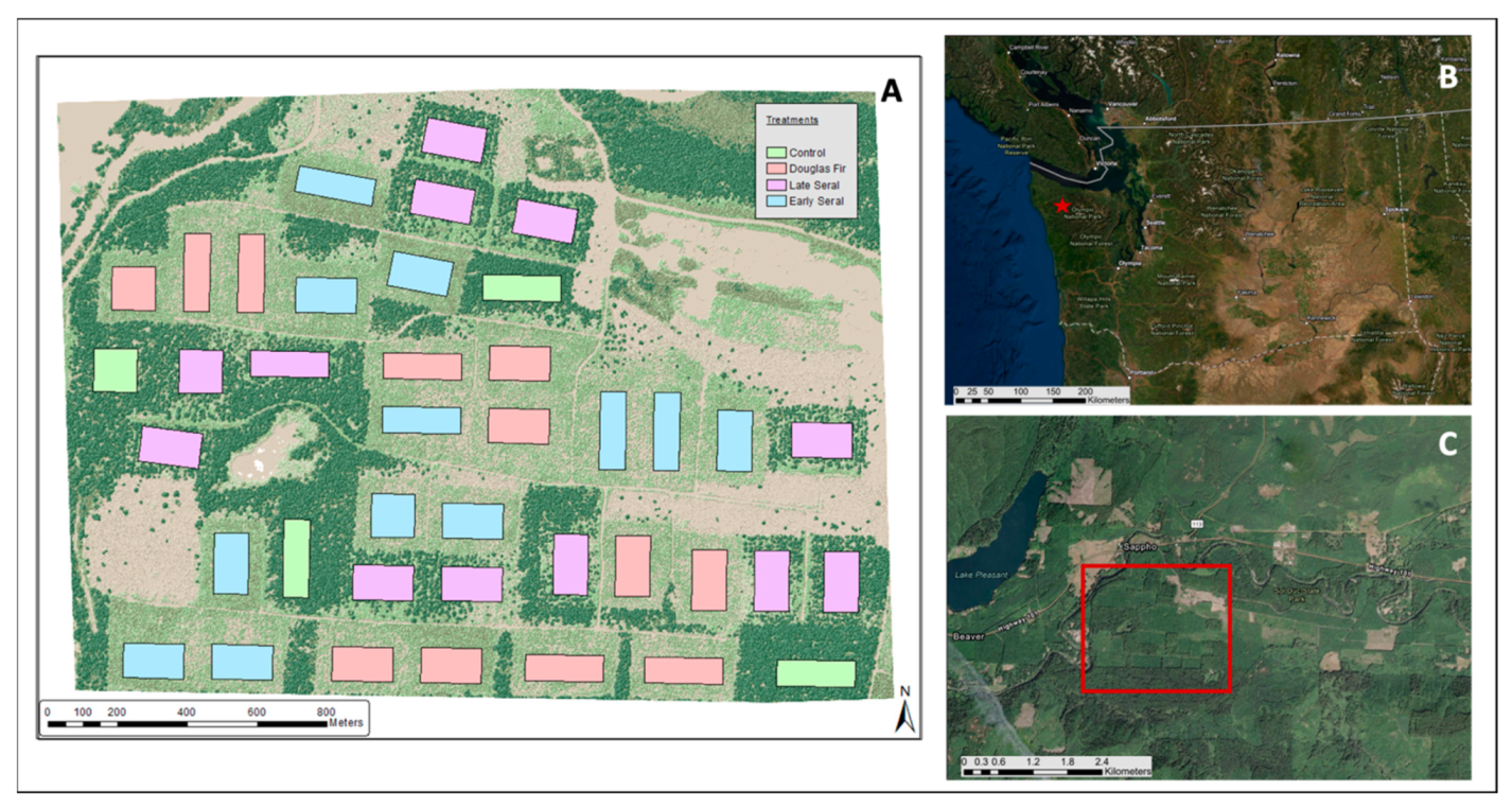
The LTEP site used in this analysis (
Figure 1) is located outside of Sappho, WA, in the northwest area of the Olympic Peninsula. The Sappho LTEP site encompasses about 416 ha and lies at about 100 m elevation on a glacial outwash plain near the Sol Duc River on the northwestern part of the Olympic Peninsula in Washington state. The site is characterized by abundant year-round rainfall (>300 cm per year), a relatively mild climate, and highly fertile soils. At this site, researchers manipulated forest structure to mimic different stages of forest development and succession by varying the level of harvesting, tree species replanted, and the amount of downed wood left behind after harvest. Two hundred tree plots, each 18 by 18 m, have been installed and measured on the Sappho site. These include 60 plots in early seral conditions created by clearcutting in 1995 and then replanting equal proportions of red alder and Douglas fir seedlings to mimic an early seral forest. We focused on these early seral plots in this study, as they typically have the largest amount of red alder.
Since the initial treatment in 1995, additional tree species have naturally regenerated in the early seral plots. Species include western hemlock (Tsuga heterophylla (Raf.) Sarg.), Sitka spruce (Picea sitchensis (Bong.) Carrière), cascara (Rhamnus purshiana (DC.) A. Gray), and vine maple (Acer circinatum Pursh). In these plots, the most common large trees (DBH 10 cm or larger) are Douglas fir, western hemlock, and red alder.
2.2. Ground Reference Data
Field data for this study were collected by a group of field technicians during the summer of 2020. Measurements were taken on 59 of the 60 early seral tree plots in the study site. One early seral plot could not be relocated. Measurements recorded for individual trees in the tree plots included species, diameter at breast height (DBH; cm) measured at a height of 1.37 m (4.5 feet), distance and azimuth from each tree to a central reference tree, and any other relevant comments regarding the condition of the tree. For example, comments were recorded if the tree was: dead, leaning more than a 45°, part of a cluster of stems sharing the same base, or growing on top of a stump.
The reference tree for each plot was picked based on the size and location of the tree within the tree plot. It needed to be large enough to be visible from all other trees on the tree plot and, ideally, located near the center of the plot. GNSS location data were collected for the reference trees using survey-grade receivers (Javad Triumph 2) and post-processed using a nearby base station. While these receivers are capable of millimeter accuracy under ideal conditions (open sky with no nearby reflecting surfaces), we typically see position errors of 1–2 m under dense canopy and occasionally see errors exceeding 5 m [
18]. The GNSS locations provided an initial location for the stem maps. Distance was measured using a standard closed reel aluminum measuring tape from the middle of the reference tree to the middle of each other individual tree located within the plot. Azimuth was measured using a standard field compass, with the field technician standing at the tree in question and measuring the azimuth to the reference tree. The distance and azimuth were used to create stem maps for each tree plot with the reference tree as the origin. These stem maps were converted into individual shapefiles for each tree plot. Individual points within the shapefile represented the base of individual trees in the plots and the fields in the associated database contained the tree attributes measured in 2020.
2.3. Plot Survey Data
Survey work related to the establishment of the Sappho LTEP site was originally completed from 1992 to 1993 by a team of professional surveyors. The survey located the plot corners but not the individual trees. Since the original survey, the coordinates for tree plots have been revised over time using a variety of different methods. However, due to the passage of time, turnover in personnel, and poor records, there is limited information regarding the original survey methods and data, and/or the methods used to revise the data. We know from recent visits by field technicians that the survey data for tree plot locations are not entirely accurate.
2.4. LiDAR Data
All LiDAR point cloud data used in this study were downloaded from the Washington State Department of Natural Resources (WADNR) LiDAR Portal. These data were acquired by the Puget Sound LiDAR Consortium (PSLC) for the WADNR from QSI Environmental [
19]. Data were acquired from 31 December 2014 to 6 March 2015. Products were delivered to the WADNR in the Washington State Plane South projection with a horizontal datum of NAD83 and vertical datum of NAVD88 and units of US survey feet. Point data were processed and classified to identify ground points by QSI Environmental. Two LiDAR sensors were used: a Leica ALS70 and a Leica ALS80. Sensors were flown at a survey altitude of 1400 m with a 30° field of view. The target pulse rate was 198 kHz and 195 kHz for the ALS70 and ALS 80 and intensity was recorded as 8-bit values. The LiDAR flights were flown with a side-lap of greater than or equal to 60%, meaning that there was an overall overlap greater than or equal to 100%. The average aggregate pulse density (first return density) was 17.26 pulses/m
2 and the average density for ground classified returns was 1.31 points/m
2. Absolute accuracy, reported as Fundamental Vertical Accuracy (FVA), for the data was 16.2 cm (1.96 * RMSE) using 96 ground control points not used in the calibration process. No horizontal accuracy assessment was reported for the data.
2.5. Combining Ground Reference Data, Field Survey Data, and LiDAR Data
We processed the LiDAR point clouds and created canopy height models (CHMs) for each tree plot in R Studio (version 4.0.4) using the lidR package (version 3.0.4) [
20]. We first normalized the point clouds using the normalize_height function. Finally, we created the CHMs using the grid_canopy function with an output resolution of 0.1524 m and the dsmtin algorithm, which is based on a Delaunay Triangulation.
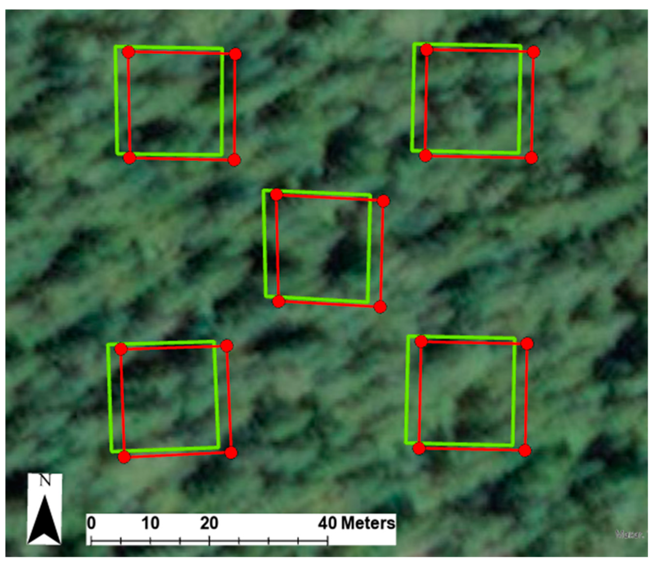
Next, we imported the processed CHMs into ArcGIS Pro (version 2.7.2), along with the stem maps and plot survey data, with the goal of matching the stem maps to individual trees visible on the canopy height models. First, we projected the stem maps and plot survey data into the coordinate system of the LiDAR data and CHMs, described previously.
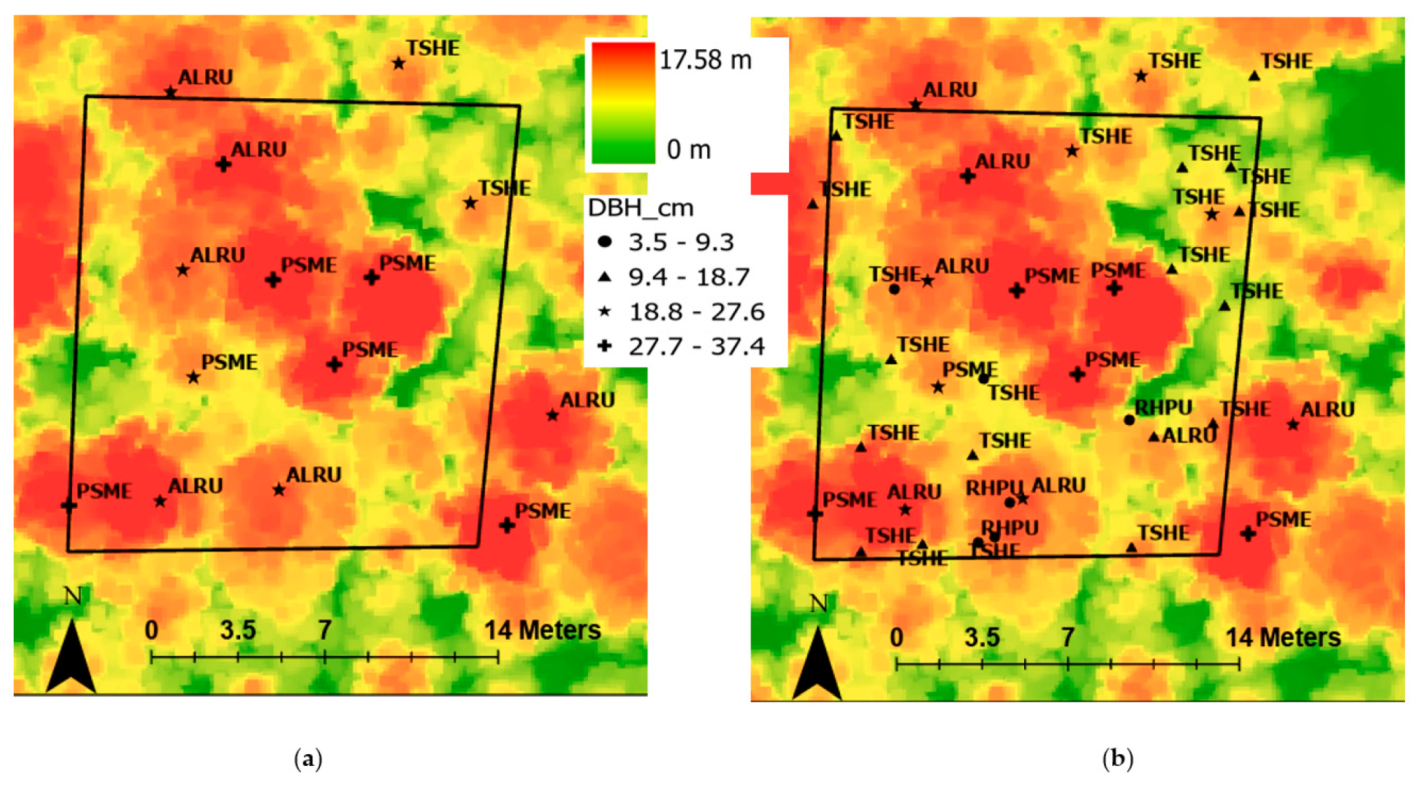
For each of the tree plots, we completed the following steps. First, we moved the entire stem map without changing the location of the tree points in relation to one another, to the general area of the intended tree plot based on the original survey data and GNSS location. Next, we filtered the stem map by DBH, temporarily removing trees 20 cm DBH and smaller. We did this because trees with a DBH of 20 cm and larger are easiest to identify on the CHMs.
Figure 2 shows an example tree plot with and without the filtering based on tree DBH. Then, we changed the symbology of the stem map points to reflect the DBH of each tree. Next, we manually adjusted the entire stem map to better align with peaks in the CHMs, matching the larger DBH sizes with the taller trees on the CHM, as well as aligning the overall pattern of the trees in the stem map to the CHM. Then, we filtered the stem map points again, adding back in the trees of DBH 20 cm and smaller. We did not attempt to adjust the locations of individual trees relative to one another. We know from field observations that most trees have some amount of lean resulting in an offset between the tree base and treetop. In addition, red alder tends to shift its crown towards canopy openings, resulting in large offsets between the positions measured on the ground and the crowns and highpoints observed in the CHM. The final step in the adjustment process was to assign an anomaly number to each tree point in the stem map.
We assigned each tree an anomaly number to help determine its suitability for use in the overall classification model; essentially, to identify mislocated or unusually growing trees so they could be removed from the dataset used to create the classification model. We assigned anomaly classification codes indicating the following conditions: no problem, dead tree, leaning tree, tree shares base with other tree/forked tree, tree is on stump, tree is less than 0.5 m away from another tree, and check tree in field (the location of the tree did not make sense, even though the locations of the surrounding trees did). We used notes taken in the field and observations of the alignment between the tree points and CHM to assign the anomaly number to each tree.
In general, we disregarded trees 10 cm DBH and under throughout this process, and we did not use them in the final classification model. We made this decision because the LiDAR data that we used were collected in 2015, but the stem maps were based on the 2020 field data. Thus, the young trees that were recorded in 2020 either did not exist in 2015 or were too small/short to be clearly visible on the 2015 LiDAR CHMs. In general, we focused on trees that were clearly visible in the CHM, hoping to maximize the quality of the data available for use in the classification model. We were confident that we had adequate data for model development and did not feel that downsizing the training dataset by removing young trees would impact the overall accuracy of the classification model [
21].
2.6. Red Alder Classification Model
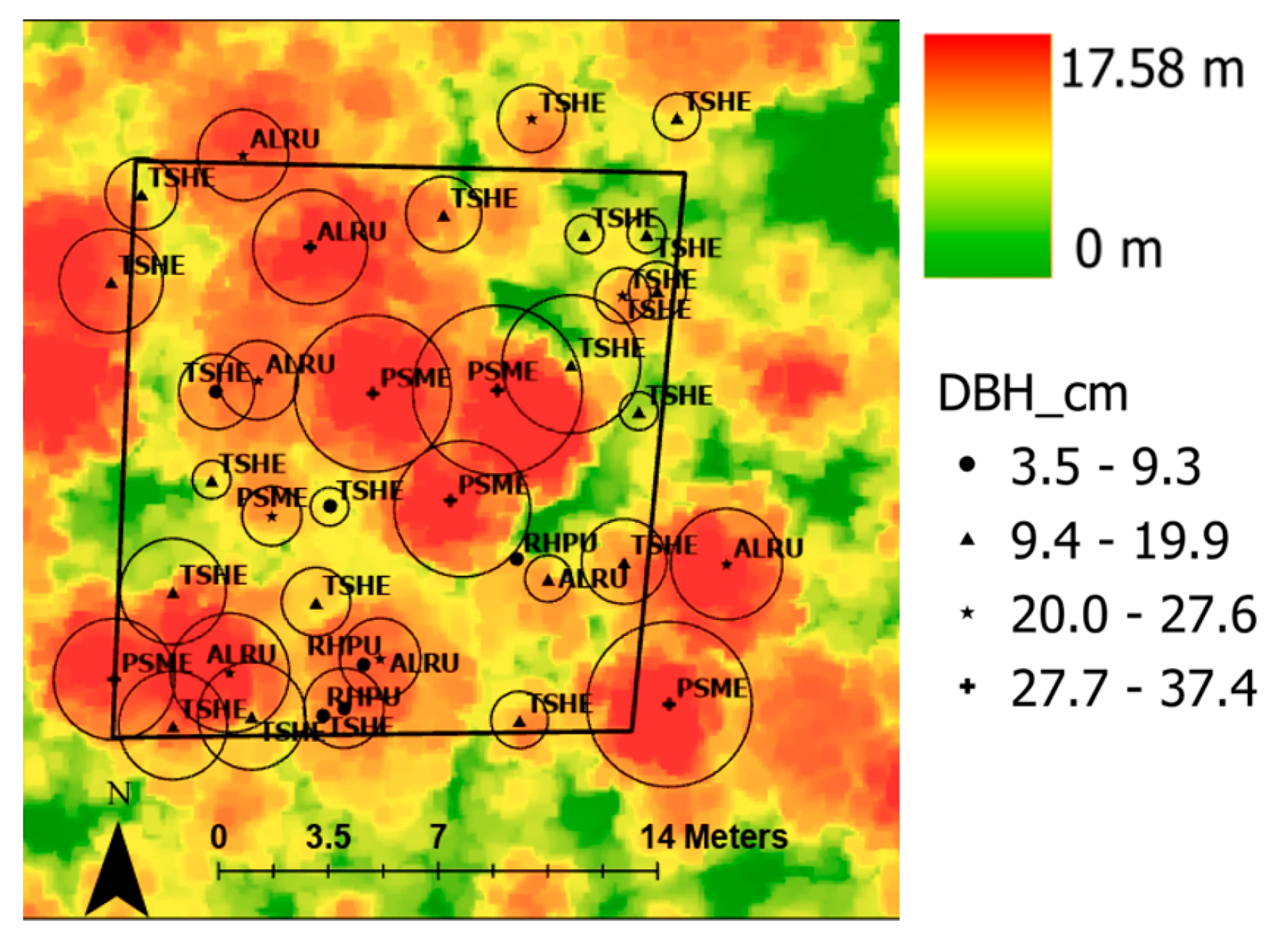
Our first step in creating the red alder classification model was determining the sample area for each tree. We opted for a simple approach and created an equation for the sample radius for each tree based on the tree height, with taller trees receiving larger circles. The equation was based on the average radius for red alder—typically the tree with the largest canopy size—and the average radius for western hemlock—typically the tree with the smallest canopy size, taken from a representative tree plot. We used the average radii divided by two, as opposed to the full radii, because we wanted to ensure that most of the LiDAR returns within each circle corresponded to the correct tree and, thus, species. We fit an equation between these two half radii averages (one for red alder and one for western hemlock) and the average tree heights for both those species. The final equation that we used was
where
r is the radius of the circle use to sample from the LiDAR point cloud and
t is the height of the tree in question. All units are in meters.
Figure 3 shows the same tree plots as shown in
Figure 2 with the addition of the circular tree crown representations.
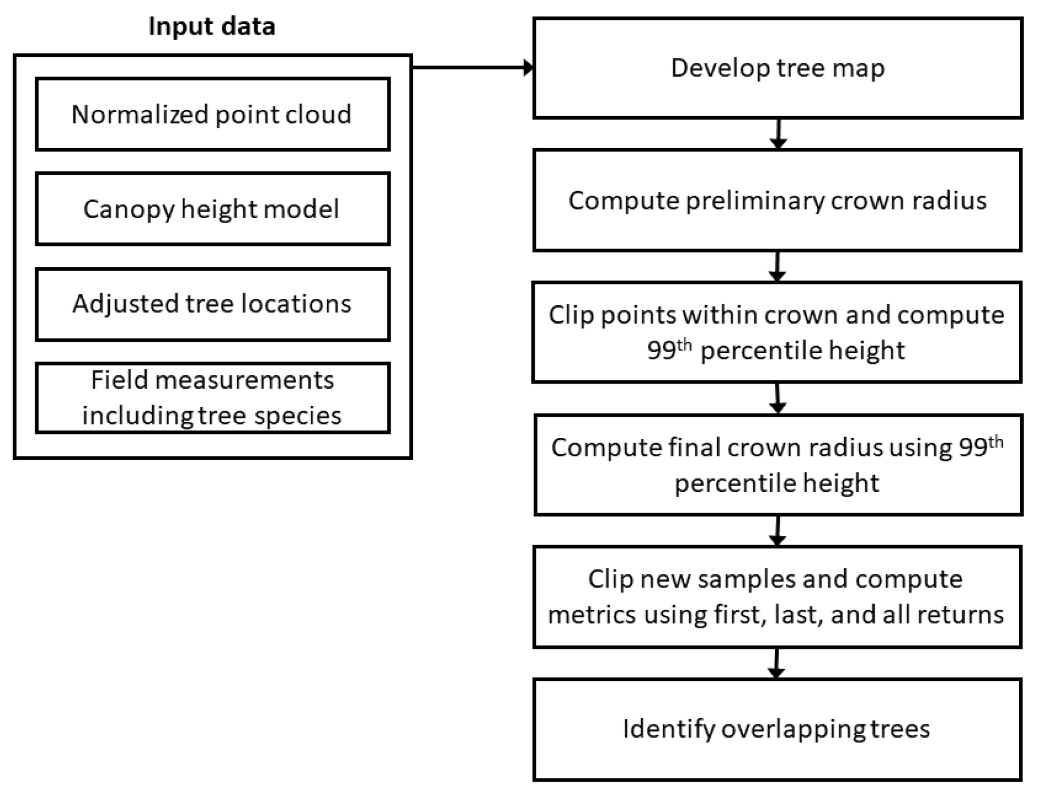
Figure 4 shows a flowchart of the process used to isolate LiDAR points for individual crowns to produce our training data. This process begins by applying the radius equation (Equation (1)) using the average height of the tallest species (Douglas fir) to produce the radius for a preliminary circular sample area around each tree. Next, we clipped the point data for the circles using the ClipData tool in FUSION (version 4.21) [
22] and then used the CloudMetrics tool to compute the 99th percentile of normalized height (P99) to use as the actual height for each tree. This actual height was then used in Equation (1) to produce a final radius for each tree. We selected P99 to eliminate the effect of unclassified or incorrectly classified outliers and returns from branches of adjacent trees. While the difference between the maximum and P99 heights was small (mean: 0.8 m, standard deviation: 1.7 m), we did find a maximum difference of 23.5 m and 55 trees where the difference was larger than 5 m. The circle radius was constrained to be at least 0.61 m (2 feet) to provide adequate LiDAR points within the sample area. We clipped a second set of points using the final circle and computed the full suite of FUSION metrics using first, last, and all returns. All intensity values used in this study were the uncalibrated, unadjusted values recorded by the LiDAR sensor and delivered by the vendor.
Using the FUSION metrics, we computed relative height and intensity percentiles for first and all returns by dividing percentile values by the 95th percentile value. Using the metrics for first and last returns, we computed several “canopy penetration” metrics as follows:
5th percentile height of last returns/95th percentile height of first returns;
10th percentile height of last returns/90th percentile height of first returns;
Mean height of last returns/mean height of first returns;
95th percentile height of first returns—5th percentile height of last returns;
90th percentile height of first returns—10th percentile height of last returns;
Mean height of first returns—mean height of last returns (hereafter called canopy penetration).
Finally, we computed two ratios using the relative height percentiles for all returns: the relative 25th percentile divided by the relative 75th percentile and the relative 10th percentile divided by the relative 90th percentile. After removing metrics not related to vegetation structure (counts of first and all returns within the circular sample), absolute maximum and minimum heights (to avoid problems with unclassified or incorrectly classified outliers), and the last-return metrics except those used to compute the canopy penetration metrics, we were left with 203 metrics for each circular sample. Knowing that individual tree crowns overlap, we wanted to identify circular clips for trees without overlap and clips for trees overlapped by the same species. We hoped that the clips without overlap would prove useful when developing the classification model. This analysis was done using the st_overlaps function in the sf package [
23] and additional variables were created for each tree indicting whether tree circles overlapped and if the overlapping circles were the same species.
The process depicted in
Figure 4 produced data for 1599 trees. We filtered the trees to remove 92 trees with anomalies identified in the field (dead trees, trees with excessive lean, and trees identified as having poor locations), 517 trees with DBH less than 10 cm, and 3 trees with insufficient points to compute metrics. In addition, we removed Sitka spruce (8 trees) and cascara (1 tree). There were no vine maple trees with DBH 10 cm or larger without anomalies. Finally, the remaining conifer species (western hemlock and Douglas fir) were grouped together and labeled “conifer”. The remaining 978 trees (150 red alder and 828 conifer) were used to develop classification models (hereafter called overlapped). Of these trees, 536 (66 red alder and 470 conifer) were not overlapped by other trees, 644 (73 red alder and 571 conifer) were either not overlapped by other trees or were overlapped by trees of the same species (hereafter called non-overlapped trees). We used the latter set of 644 trees to develop an alternate set of classification models.
Both sets of tree data, overlapped and non-overlapped, were split into training (70%) and testing (30%) subsets. Preliminary models were developed using all 203 predictors with the randomForest function in the randomForest package [
24]. We had many times more conifer species than red alder, so we balanced the sample sizes using the sampsize argument of the randomForest function with value set to the number of red alder trees in the training data sample. We also created models based on simple threshold values to better understand how individual variables performed for classification. Threshold values were computed for each variable as the mean of the median values for each type.
After developing the preliminary random forest models, we used variable importance scores produced by random forest to help select a subset of predictors and then developed additional models using the subset. We evaluated all models using the testing data (30%) and all data and selected a final model based on the overall classification accuracy using all data. For random forest models, the same set of variables was used to fit models 30 times using different random number seeds for the data split and model fit. The overall accuracy was averaged for the 30 resulting models.
The final model was applied to map the presence of red alder by first computing metrics for the entire study area using a 1.524- by 1.524-m (5 by 5-foot) grid and the first, last, and all returns within each grid cell using FUSION’s AreaProcessor workflow tool. The final model was applied using a selected subset of variables and the AsciiGridPredict function in the yaImpute package [
25].
A “forest mask” (using the same 1.524- by 1.524-m cells) was developed to identify forested areas. Cells were considered forest and assigned a value of 1 if they contained at least 10% cover (ratio of first returns above 1.37 m (4.5 feet) to total first returns) and had a 99th percentile height (all returns) value greater than or equal to 3.05 m (10 feet). Cells not meeting these criteria were assigned a value of 0. This mask was applied to the final prediction layer to eliminate non-forest areas.
4. Discussion
In this study, we wanted to improve the position data for plots and individual trees, and we wanted to map red alder over our study area to assist with another project investigating the effect of red alder on the abundance and growth of understory plants. Overall, we accomplished both goals.
We found that LiDAR canopy height models (CHMs) can be used to match individual second-growth trees with ground reference data, and we outline the methodology we used. Because we had high-quality ground reference data, and because we removed any trees with potential outliers, we can say with a relatively high degree of certainty that the LiDAR point returns used in the classification model belong to the species identified in the field. We did this by manually matching the stem maps to CHMs. We found the manual, human-based alignment process was ideally suited to our situation and speculate that it may be appropriate for other field experiments that only take field measurements on small parts of their study area. Similar types of experiments can use their field data as reference data to make a LiDAR-based model that can be applied to the rest of the experiment, or to increase the accuracy of the coordinates of their experimental plots.
Additionally, like Liang et al. [
8], we found that the separation between first and last returns was a useful metric to separate deciduous trees from conifers using data collected in leaf-off conditions. Liang et al. [
8] used two threshold values and observed overall accuracy of 89.83%. The first threshold was the proportion of pulses where the difference between the first and last return heights was significant and the second was the height difference used to determine whether the difference was significant. We simplified our canopy penetration metric to the difference in height between the mean of first and last returns within each crown and established a single threshold value as the mean of the median values for red alder and conifer species. Overall accuracy for our simple threshold model using this single metric was 88.04%, which is like the accuracy reported in [
8].
In general, overall accuracy was slightly lower when the model was trained using trees with crowns not overlapped by other tree crowns or overlapped by trees of the same species. The overall accuracy reported by random forest was slightly higher for models fit using non-overlapped trees, but the overall accuracy was lower when the model was evaluated using all non-overlapped trees or all trees including those overlapped. For the conditions over our study area, canopy densities are high. Based on our tree data, about 66% of the trees with DBH larger than 10 cm were either not overlapped by other trees or were overlapped by trees of the same species. However, this overlap determination was done using conservative circular samples. It is likely that the horizontal projection of the crowns is larger than our sample circles so more trees will overlap than indicated by our analysis. We also expected that a significant proportion of the 1.524 by 1.524 m cells used to map the species types would represent more than one species. In general, we felt using the overlapping trees to fit the models produced a model better suited for mapping species over the entire study area.
Out of a total of 1599 trees measured on our plots, 978 overlapped and 644 non-overlapped trees (see
Section 2.6 for definitions of overlapped and non-overlapped) were identified to fit and test our classification model. The random forest model with the best overall accuracy (95.68%) used the 978 overlapped trees. This sample size is considerably larger than those used in [
7] (377 trees) and [
8] (295 trees) but smaller than that used in [
9] (1413 trees) and [
21] (13,298 trees). Data were split into training and validation (also called testing) using a ratio of 70% (training) and 30% for testing. While this ratio is somewhat arbitrary, we fit and tested models 30 times using different subsets for model training and observed only small changes in the accuracy. In addition, Korpela et al. [
21] reported the results of tests of the ratio of training to testing data (training data ranging from 2.5–30%) with random forest and found only slight differences in accuracy (<1% differences overall for the three species being classified). However, the number of trees used in [
21] was much higher than our study (13,298 trees in [
21]) so these results may not apply to our study.
Our results show that LiDAR-derived metrics can be combined with field data to make a useful training dataset provided you have accurate locations for individual trees. Our classification model was able to identify red alder and conifer species with high (95.68%) accuracy. We applied this model using a raster with 1.524 m by 1.524 m cells, which represents an area that is about the same as the average crown size for the trees. However, this is still a relatively large area and could contain multiple species. While our goal for this work was to identify red alder to provide information to support additional studies regarding the relationship between red alder and understory shrub species, our methods may be suitable for identifying other species. We did explore, using the same random forest modeling approach, separating Douglas fir and western hemlock. The preliminary results were promising but further evaluation and model refinements are beyond the scope of the work presented here. While we expect the same methodology will work for additional species, different LiDAR metrics will likely prove to be more useful than those used in our red alder model. Our LiDAR data were collected in late winter and early spring (mostly January and February). Red alder flowers in February-March so it is likely that catkins were forming during the LiDAR data collection period. This may have produced a somewhat unique “signature” for red alder trees manifested through the point cloud metrics. Efforts to identify additional species may rely more heavily on metrics describing the vertical distribution of returns rather than the intensity and penetration metrics that we used for red alder.
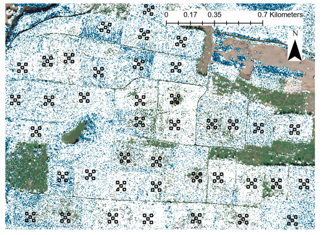
We applied our classification model to an area (3025 ha) much larger than the Sappho site (416 ha) and compared the results to aerial imagery from 2016 (LiDAR data were collected in 2014–2015) (
Figure 8). In general, the classification results identified red alder stands and scattered individual red alder trees across the broader area. Riparian areas known to have stands dominated by red alder were identified correctly along with additional treatment areas, not used in this study, within the Sappho site known to have a high proportion of red alder. While no formal validation was conducted for the area outside the Sappho site, visual evaluations indicate that the classification model performed well.
We were somewhat surprised that no LiDAR metrics related to the distribution of return heights proved useful for our final classification model. Our final model relied on our penetration metric that relates to the porosity of the canopy and intensity metrics. We performed a visual examination of the circular point-cloud clips for trees produced using our somewhat conservative approach to estimate the sample radius and found that there were no morphological features evident to distinguish species. Our study area can be characterized as having a dense canopy with closely spaced trees so there is overlap between most tree crown perimeters. While our circular samples produced data representative of the canopy for our field-measured trees, the clips do not provide easily interpreted information regarding the crown shape, crown profile, or the arrangement of branches and foliage. In hindsight, this could explain why no height distribution metrics proved useful for the final classification model.
Our methods are not without limitations. To duplicate our methods, ground studies must collect position data for field plots and tree stems (relative to a local reference point for each plot) to provide a starting point to align the stem maps with the CHMs. These locations need to be within 5 to 10 m of the true plot locations. Such accuracies are possible with mapping-grade GNSS receivers [
18]. In addition, our study area was relatively small, and involved a single forest type at a specific stage of development. More robust methods may be needed for more complex forest types.
Our alignment process relied on manual adjustments to the overall stem map for each plot. This was practical given the size of our study area and the number of plots. An automated process is possible. However, given that most trees exhibit some lean or an offset between the stump and treetop (highpoint) locations, it may be necessary to select a subset of trees to use with an automated alignment process. Automated alignment is further complicated by the habit of red alder to shift their crowns to capture light. It is not uncommon to see an offset of several meters between the stump location and the highest point of the crown. The best solutions would likely involve extracting individual tree objects from the point cloud, detecting stems, and using stem locations along with field locations in an automated process (like the process using terrestrial laser scanning data reported in [
27]). However, the point density of the LiDAR data and the dense overstory did not provide sufficient data to detect all stems with confidence. Given the size of our study area and the number of plots involved, we felt a manual adjustment process produced the best locations for all the trees on the plots.
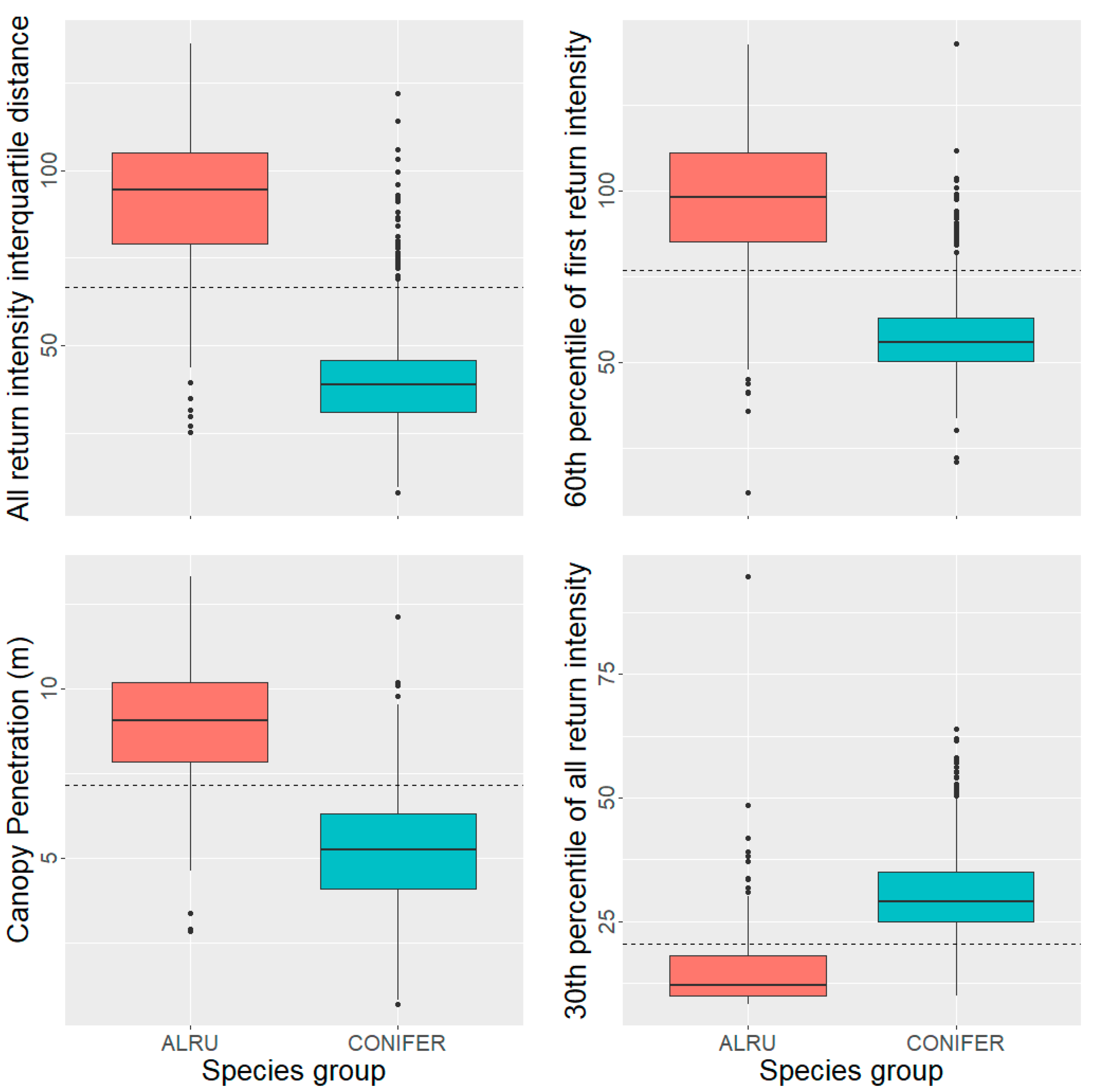
Furthermore, intensity values used in our study were the uncalibrated, unadjusted values recorded by the LiDAR sensor and delivered by the vendor. Metrics used in our classification model included intensity for first returns (First.Int.P60) and intensity for all returns (Int.IQ and Int.P30). While many studies also use the “raw” intensity values [
7,
8], studies that employed range normalization and corrections to reduce the effect of automatic gain control (AGC) report higher classification accuracies using the adjusted values [
28]. Our model might be improved by using adjusted intensity values. However, improvements in accuracy would likely be minimal.
For our classification model, our variable selection process was not perfect. The selected variables were not those with the highest importance scores, but they were among the variables with the highest scores. We experimented with methods to select a subset of variables, but none performed better than the subset described in the results. Many of the LiDAR metrics were correlated. Random forest performs well using data with highly correlated variables, but the resulting importance scores can be misleading. In the end, variable selection was somewhat subjective using the importance scores produced by random forest and the accuracies of the simple threshold models as guides to select the final subset of variables.
Future research for this classification model includes combining it with other types of remote sensing technology, such as four-band (RGB and near-infrared) imagery and satellite imagery. Additional research includes using the same model development approach to classify Douglas fir and western hemlock, in addition to red alder. Lastly, as stated in our objectives, we want to use the results of the classification model to explore the relationship between the presence or absence of red alder and understory species diversity.


