Article

Retrieving the Infected Area of Pine Wilt Disease-Disturbed Pine Forests from Medium-Resolution Satellite Images Using the Stochastic Radiative Transfer Theory

1
Research Center of Forest Management Engineering of State Forestry and Grassland Administration, Beijing Forestry University, Beijing 100083, China
2
Institute of Geography, Henan Academy of Sciences, Zhengzhou 450008, China
3
Northwest Surveying and Planning Institute of National Forestry and Grassland Administration, Xi’an 710048, China
4
Key Laboratory of National Forestry and Grassland Administration on Ecological Hydrology and Disaster Prevention in Arid Regions, National Forestry and Grassland Administration, Xi’an 710048, China
5
Beijing Key Laboratory for Forest Pest Control, Beijing Forestry University, Beijing 100083, China
*
Author to whom correspondence should be addressed.
Remote Sens. 2022, 14(6), 1526; https://doi.org/10.3390/rs14061526
Submission received: 20 January 2022 / Revised: 3 March 2022 / Accepted: 17 March 2022 / Published: 21 March 2022
(This article belongs to the Special Issue Forest Disturbance Monitoring Using Satellite Remote Sensing)

Abstract

:
Pine wilt disease (PWD) is a global destructive threat to forests which has been widely spread and has caused severe tree mortality all over the world. It is important to establish an effective method for forest managers to detect the infected area in a large region. Remote sensing is a feasible tool to detect PWD, but the traditional empirical methods lack the ability to explain the signals and can hardly be extended to large scales. The studies using physically-based models either ignore the within-canopy heterogeneity or rely too much on prior knowledge. In this study, we propose an approach to retrieve PWD infected areas from medium-resolution satellite images of two phases based on the simulations of an extended stochastic radiative transfer model for forests infected by pests (SRTP). A small amount of prior knowledge was used, and a change of background soil was considered in this approach. The performance was evaluated in different study sites. The inversion method performs best in the three-dimensional model LESS simulation sample plots (R2 = 0.88, RMSE = 0.059), and the inversion accuracy decreases in the real forest sample plots. For Jiangxi masson pine stand with large coverage and serious damage, R2 = 0.57, RMSE = 0.074; and for Shandong black pine stand with sparse and a small number of single plant damage, R2 = 0.48, RMSE = 0.063. This study indicates that the SRTP model is more feasible for pest damage inversion over different regions compared with empirical methods. The stochastic radiative transfer theory provides a potential approach for future monitoring of terrestrial vegetation parameters.

1. Introduction

Pine wilt disease (PWD) is a global destructive threat to forests which is caused by the pine wood nematode (Bursaphelenchus xylophilus) and is spread through an insect vector through the pine sawyer beetle (Monochamus spp.). PWD was first recorded in North America [1] and has been widely spread all over the world, especially in East Asia [2,3]. Since the first appearance in 1982 in Nanjing, China, PWD has been the most catastrophic pine disease and has caused severe tree mortality in China [2,4]. It is a very important issue for forest managers to detect the infected area in a large region and wipe out the damaged trees to prevent the spread of PWD. Therefore, it is imperative to establish an effective method to accurately monitor and map infected areas of PWD.
The optical property changes of pine crowns after PWD infestation makes it possible to identify infected trees. These changes are caused by changes in physiological, biochemical parameters and leaf structure impacted by PWD. The visible discoloration of infected needles generally takes place from green to light green, yellow to red [5]. In severely damaged areas, it is quite common to find the forests are mixed with green and red crowns. Such damage pattern makes it feasible to distinguish the infected regions to assess the forest damage and construct measures of management.
Remote sensing is considered a potential approach to detect forest pest and diseases [6,7,8,9]. Among different types of sensor loads, medium satellite remote sensing, such as that provided by Sentinel-2, provides large-area and multi-temporal information for land surface, information which is a feasible tool for forest monitoring at a larger scale. The theoretical foundation used in most previous studies on the assessment of forest pest damage by remote sensing regarded image processing techniques and empirical algorithms [10]. For instance, the infected parts and healthy parts of forests were differentiated by setting thresholds to specific spectral indices such as the red–green index (RGI) [11], the normalized difference vegetation index (NDVI) [12], the normalized difference moisture index (NDMI) [13,14], the disturbance index (DI) [15], and the enhanced wetness difference index (EWDI) [16]. The infected regions were identified by image classification techniques with the assumption that new land-cover types should be assigned to infected forests on account of their distinctive symptoms [17,18,19,20,21]. Quantitative machine learning models such as statistical regression were widely used to build correlation between image-derived predictor variables and field-measured damage indicators [22,23,24,25]. With the time-varying information from multi-temporal data, the infected areas were retrieved by coupling the empirical algorithms with change detection techniques [26,27,28,29]. These empirical approaches cannot consider the mechanism of the spectral response to vegetation stress. In complicated forest scenarios, the information carried by stress is always mixed with other factors, and the mix pattern varies with different study areas. Consequently, these methods lack the ability to explain the signals and can hardly be extended to large scales. On the other hand, the quantitative empirical models are very dependent on the training samples. The chosen training samples should be representative of the study area. Too few training samples may reduce the accuracy of the prediction model and too many training samples is labor-consuming. Hence, more physically-based methods need to be developed for accurately retrieving the infected area at large scales.
Some studies have utilized radiative transfer models to detect forest pest and diseases using simulations. For example, leaf incorporating biochemistry exhibiting reflectance and transmittance yields (LIBERTY)—a leaf model—and invertible forest reflectance model (INFORM)—a canopy model—were coupled to detect pine shoot beetle (PSB) stress in Yunnan Pine forest [30]. One-dimensional (1D) radiative transfer (RT) models are not qualified enough to accurately retrieve the damage level of PSB damage [31], the three-dimensional (3D) Radiosity Applicable to Porous IndiviDual Objects (RAPID) model was used to estimate PSB damage. The incidence of Xylella fastidiosa infection in olive orchards was monitored using ground-based evaluations, airborne imaging spectroscopy and Sentinel-2 time series through 3-D radiative transfer model FLIGHT [32]. The shortcomings of such studies with physically-based models include: (1) the fact that, in most studies, the leaf elements in the models are homogeneous and linearly mixed with healthy and damaged leaves preventing the scattering between healthy and damaged leaves from being accurately implemented and; (2) that most of these used high-resolution data to provide prior knowledge. It is not always feasible to obtain sufficient knowledge in large-scaled mapping. The results need to be further tested when the data source is limited. In our previous study, we proposed a model for simulating bi-directional reflectance factor (BRF) of forests infected by pests based on the stochastic radiative transfer (SRT) theory [33], which is referred to as SRTP hereafter. In this model, tree crowns are modeled as identical geometry shapes, with healthy and damaged crowns randomly distributed in the scenario. Doing this parameterizes the damage level of a heterogeneous canopy in a simple way. This model is balanced between accuracy and computational efficiency, which has potential in forest damage inversion but has not been tested by present.
In this work, we chose the PWD-disturbed pine forests as a case study and tested the applicability of SRTP in damage area inversion. The main objectives of this study were (1) to propose an approach to retrieve forest pest damage areas from satellite images using SRTP simulations with a small amount of prior knowledge, and (2) to evaluate the performance of the inversion approach in different study sites. To overcome the insufficiency of prior knowledge for complicated forest scenes, images of both healthy and infected phases were used to detect the changes caused by PWD. To provide sufficient sample plots to validate the approach, realistic scenarios simulated by 3D models were used as well as field data, because 3D RT models working with more realistic crown architecture have been considered to have more accurate simulations of complex RT processes for heterogeneous canopies [34,35].

2. Materials and Methods

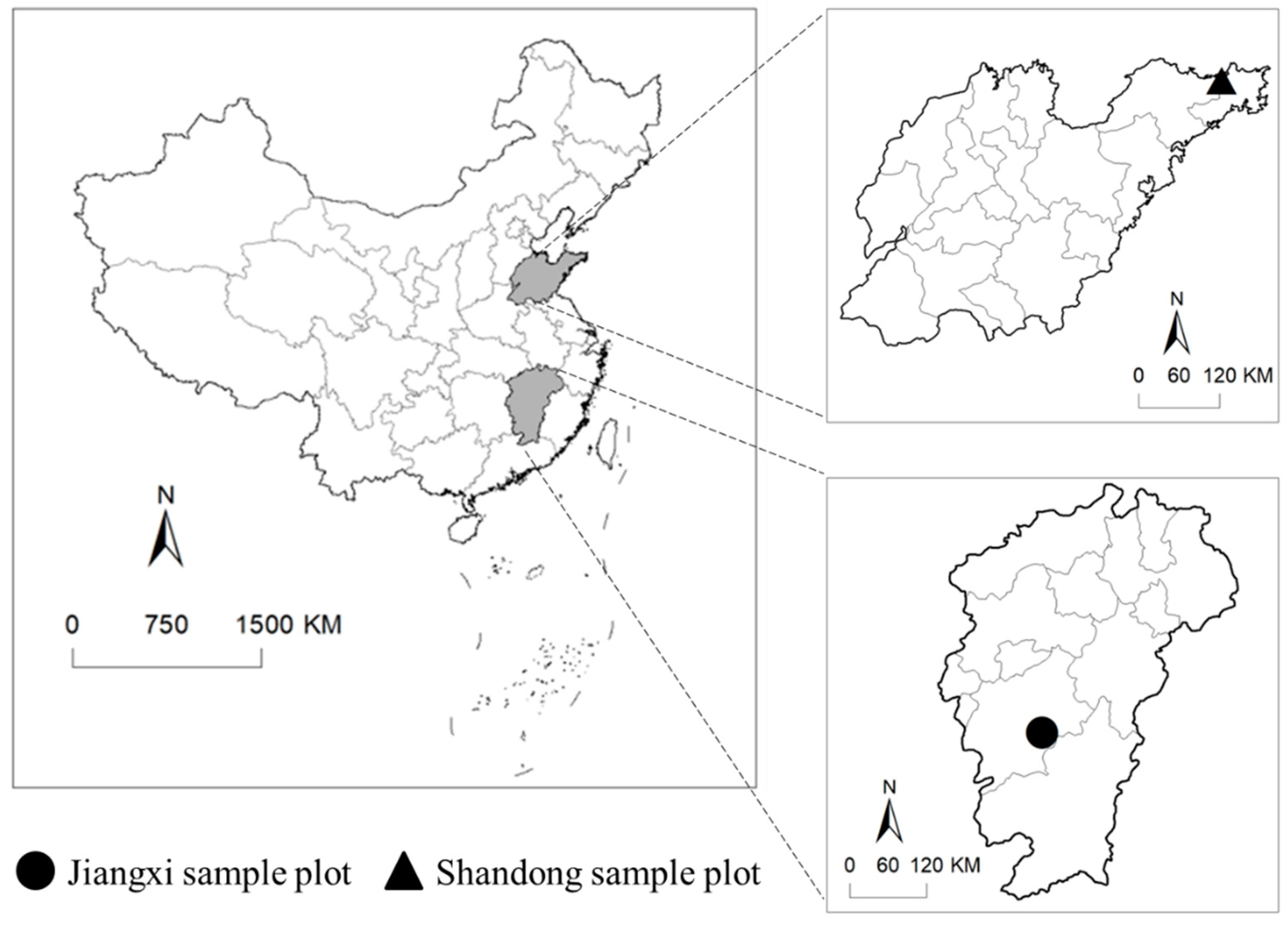
2.1. Field Data and Sample Plots

The leaf reflectance of healthy and damaged needles, the diameter and height of crowns and the soil reflectance were each measured in the field campaign as prior knowledge. The forest sample plots in this study included two categories: plots simulated by 3D models and plots established by field campaign. The simulated plots were generated by large-scale remote sensing data and image simulation framework over heterogeneous 3D scenes (LESS) [35]. The field plots were acquired from unmanned aerial vehicle (UAV)-based measurements of forests infected by PWD in Jiangxi and Shandong provinces, China.

2.1.1. Study Area and Field Data

In this study, two pine species in different regions of China were investigated. The first one is masson pine (Pinus massoniana Lamb.) in Taihe, Ji’an, Jiangxi province, China. The second is black pine (Pinus thunbergii Parl., also named as Japanese black pine) in Muping, Yantai, Shandong province, China (Figure 1). The study site in Jiangxi is located in Jitai basin which belongs to mid-subtropical monsoon humid climate (26°44′N, 115°4′E). PWD in the masson pine forests often breaks out in summer and autumn when the climate is hot and dry. The study site in Shandong belongs to continental climate in the Temperate East Asian monsoon region, which is obviously affected by the ocean (37°20′N, 121°49′E). As one of the major tree species, the black pine forests always get infected by PWD in the early summer. Generally, incidence of PWD is related to high temperature and drought. From mid-September to early-November in China there are more clear skies and significant symptoms of red crowns. We investigated the forests of Shandong in September and Jiangxi plots in November by keeping a similar air temperature in the two climate zones.
The reflectance and transmittance of healthy and damaged needles, the branch reflectance, and the diameter and height of crowns were measured in the field campaign as prior knowledge. There were four groups of needle samples: healthy or damaged masson pine needles in Jiangxi, healthy or damaged black pine needles in Shandong. For each group, 50 needles and 10 branch samples were collected and brought to the laboratory. Masson pine needles were between 10 cm and 18 cm in length, and about 1 mm in diameter; black pine needles were between 6 cm and 13 cm in length, and about 1.5 mm in diameter. Needle reflectance and transmittance and branch reflectance for each needles sample was measured using ASD FieldSpec3 (350–2500 nm, 3 nm spectral resolution, 1.4 nm sampling interval) in a dark room. Transmission Dip Probes were set on the light source and used to measure the needle transmittance. The reflectance and transmittance of healthy and damaged needles of masson pine and black pine needles are depicted in Figure 2. The tree crown structural parameters of black pine were measured in Shandong, including diameter at breast height (Dbh), tree height (H), crown base height (Hc), crown width (D), crown height (L). A total of 175 trees were measured, in which D was calculated from the mean crown width in the north–south direction and in the east–west direction. The surveyed 175 trees were located within two 30 m × 30 m sample plots in Shandong that were about 5 km apart from each other. Since there is no regular difference observed between masson pine and black pine trees in crown shape, the crown structural parameters collected in Shandong were used for both species.
The UAV data were obtained from field campaigns to acquire the prior knowledge on the forest canopies in Jiangxi and Shandong province, China. A Phantom 4 Multispectral UAV with an RGB sensor and five monochrome sensors (center wavelengths: 450, 560, 650, 730, 840 nm) was used to investigate the forests. In each site, the flight was conducted twice including the healthy phase and the damaged phase. The first flight was in May in Jiangxi and in June in Shandong. The second flight took place in November in Jiangxi and in September in Shandong. The multispectral images were acquired by the sensor with the vertical downward observation mode, of which the focal length is 5.74 mm and angular field of view is 62.7°. The UAV collected images at a flight height of 60 m with 80% across-track overlap between the two nearest flight lines. All images were orthorectified by Pix4D software and radiometrically calibrated to convert the radiance values to reflectance by a carpet reference. Four ground control points in each flight were used to perform geometric accuracy correction of the mosaic multispectral image. The final pixel size of the corrected image is 0.05 m.
The soil reflectance was extracted according to the regions in UAV data (i.e., bare soil and vegetation-covered soil), while 15 + 15 regions were selected from the Jiangxi and Shandong UAV images containing pure pixels of typical kinds of soil. For each region, the average reflectance could be calculated from the corresponding pixels in the satellite images. Finally, 30 pairs of soil reflectance for two phases were used as input.

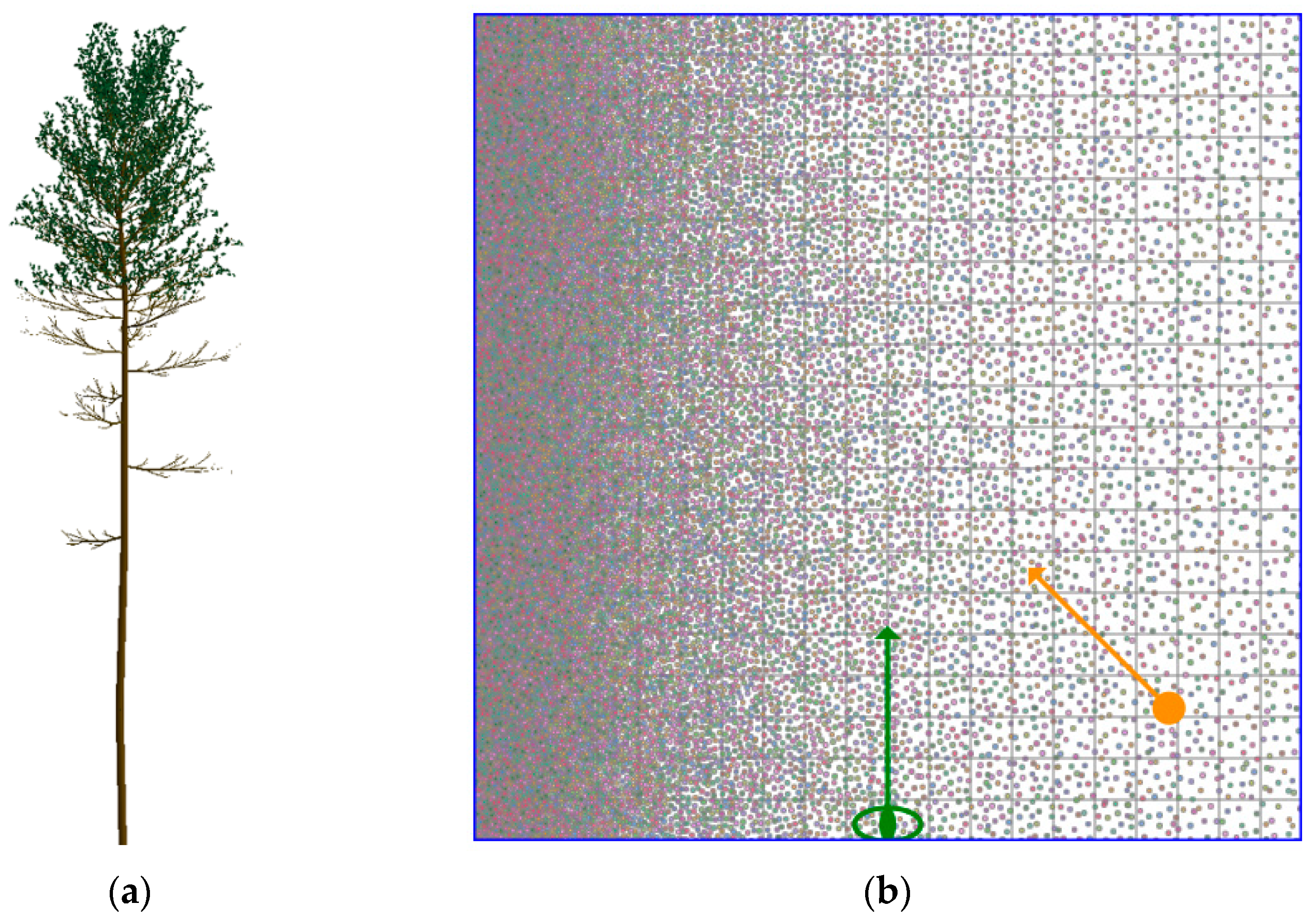
2.1.2. Simulated Sample Plots

Because of the difficulties of getting enough measured plots, the simulated plots were used to evaluate the performance of different scenes. The simulated plots were generated by the following steps: (1) A tree obj-file that is similar to pine tree was chosen to denote an individual tree. The crown diameter was set as 4 ± 0.4 m and the tree height was set as 18 ± 1.8 m (Figure 3a). (2) Four 900 m × 900 m plots were generated by LESS. (3) Each plot was divided into ten 900 m × 90 m subplots according to the amount of trees, with the canopy coverage ranging from 0.1 to 0.95. The trees were randomly generated within each plot (Figure 3b). (4) The trees were composed of healthy and damaged trees. The trees were chosen as damaged trees by a random probability in each plot. The random probabilities of the four plots were set as 0.25, 0.5, 0.75 and 1. The input reflectance spectra of healthy and damaged leaves were set randomly within the ranges of 1 ± 3% of the measured spectra in Figure 2. (5) The four 900 m × 900 m plots were finally divided into 3600 30 m × 30 m plots. The soil was heterogeneous for each plot which was randomly based on the UAV-extracted soil spectra.
The canopy coverage, LAI, infected area of each plot could be calculated in LESS. The damaged trees were changed into healthy trees to generate the healthy plots corresponding to the healthy stage of the 3600 plots.

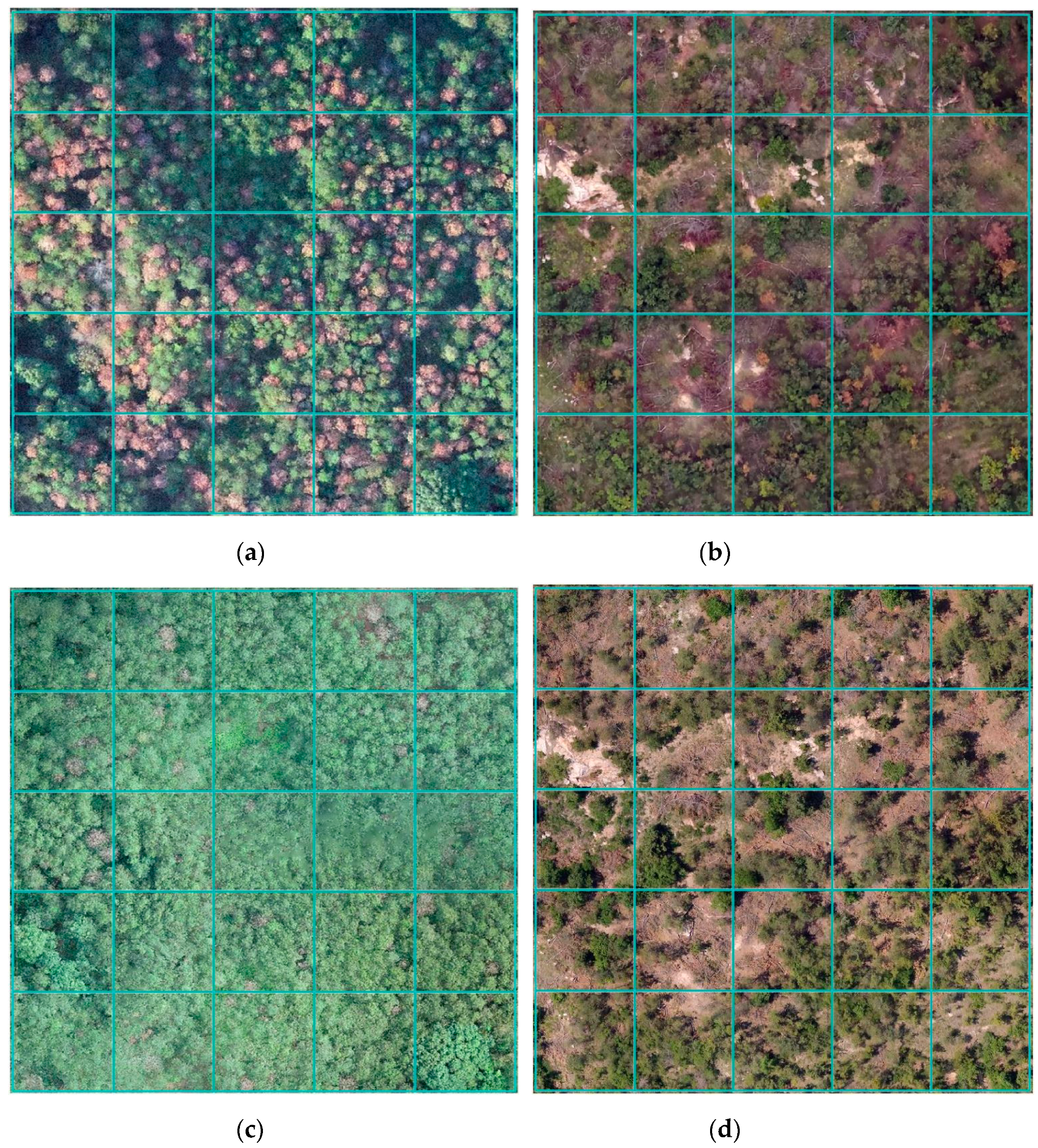
2.1.3. Field Sample Plots

Other than simulated plots, field plots in Jiangxi and Shandong provinces were established to validate the inversion model in real forests. In each of the UAV images of Jiangxi (Nov.) and Shandong (Sep.), we chose a typical 150 m × 150 m infected pine plot. Each plot was divided into 25 30 m × 30 m plots. A total of 50 plots were established (Figure 4a,b).
It is difficult to acquire the precise area of damaged crowns only by field measurements. Due to the high resolution of UAV images, the healthy trees and damaged trees were visually distinguishable. We used the supervised classification approach in ENVI software to extract the infected area of each plot. For the trees that were hardly distinguished, we modified the classification results according to the field investigation.
In the UAV images of Jiangxi (May) and Shandong (June), 50 plots at the same location were established as the corresponding healthy plots (Figure 4c,d).

2.2. Satellite Remote Sensing Images

2.2.1. Image Acquisition

Corresponding to the size of 30 m × 30 m plots, two types of remote sensing images with the same resolution were used for inverting infected area of PWD. The first type is the images simulated by LESS; the second is the 30 m resolution images resampled from Sentinel-2 images. The hyperspectral images with 0.5 m spectral resolution were simulated using the four 900 m × 900 m plots by LESS, in which the solar zenith and azimuth angles were 30° and 135°, respectively, and the view zenith angle was 0°. By both spectrally and spatially resampling using the spectral response functions of Sentinel-2, multi-spectral images at 30 m resolution were finally generated. The Sentinel-2 2A images of the study sites were downloaded in the Google Earth engine. The bands of LESS-simulated images were the same as the bands of Sentinel-2. The Sentinel-2 images were resampled for two reasons: (1) In 10 m × 10 m plots, the shadow effect from neighboring pixels on the edge of the target pixel is too large, which might increase errors. (2) In SRT theory, the canopy structure is parameterized by stochastic probability functions, too few trees might cause bias with the stochastic results. For each of the two types, the images of both healthy and damaged phases were simulated or downloaded.

2.2.2. Construction of Spectral Indices

With reference to relevant previous research results, A total of 10 spectral indices established by bands of Sentinel-2 that are commonly used in vegetation dynamic change monitoring were selected as the spectral features for predicting the infected area of PWD. The vegetation spectral index calculation method is shown in Table 1. Note that B3, B4, B5, B6, B7, B8 and B8a represent the corresponding bands of Sentinel-2 (center wavelengths: 560, 665, 705, 740, 783, 842, 865 nm). All 10 indices were calculated on each pixel (30 m by 30 m) in both simulated and real Sentinel-2 images. The spectral indices of both healthy and damaged stages were calculated to indicate the changes of image features.

2.3. SRTP Model

2.3.1. Model Description

The SRT theory was developed from the classic 3D radiative transfer [42] which was originally solved for the radiation regime in each location of the 3D scene [43]. To focus on the average over satellite pixel radiation for the remote sensing applications, the SRT model averages the 3D radiative regime into a 1D form, and provides the equation directly for the mean radiation field [44]. Based on the statistical techniques of the SRT theory, the averaging procedure is addressed by the parameterization of equation in terms of two stochastic moments of the vegetation structure. The SRTP model is an extension and application of the SRT theory in forests infected by pests [33]. For a damaged forest modeled by SRTP, the foliage was divided into a healthy foliage class and an infected foliage class. The first stochastic moment is the probability, p(i)(z), of finding foliage class i at canopy depth z, which is responsible for the horizontal heterogeneity of the canopy; and the second moment is the pair–correlation function, q(i,j)(z,z′,Ω), between foliage class i at canopy depth z and foliage class j at depth z′ along the direction Ω, which can describe the vertical heterogeneity of the canopy. The SRTP equations for damaged canopies followed the SRT model with species mixture [45]:
I ( z , Ω ) + 1 μ j z p ( j ) ( z ) σ ( j ) ( Ω ) U ( j ) ( z , Ω ) d z = 1 μ j z ω 0 ( j ) d z 4 π p ( j ) ( z ) U ( j ) ( z , Ω ) σ S ( j ) ( Ω Ω ) d Ω + I ( z B , Ω )
U ( i ) ( z , Ω ) + 1 μ j z K ( i , j ) ( z , z , Ω ) σ ( j ) ( Ω ) U ( j ) ( z , Ω ) d z = 1 μ j z ω 0 ( j ) d z 4 π K ( i , j ) ( z , z , Ω ) U ( j ) ( z , Ω ) σ S ( j ) ( Ω Ω ) d Ω + U ( i ) ( z B , Ω )
K ( i , j ) ( z , z , Ω ) = q ( i , j ) ( z , z , Ω ) / p ( i ) ( z )
where I(z,Ω) and U(i)(z,Ω) are the mean radiation intensity averaged over the total horizontal space and over portion of plane occupied by foliage class i, respectively. I(zB,Ω) and U(i)(zB,Ω) represent the corresponding boundary conditions. μ is the cosine of polar angle in direction Ω. σ(j)(Ω) denotes the total extinction cross-section of the foliage class j, and σS(j)(Ω′⟶Ω) stands for the differential scattering cross-section from direction Ω′ to Ω. ω0(j) is a wavelength-dependent term standing for the single scattering albedo of each foliage class. K(i,j)(z,z′,Ω) indicates the conditional pair correlation of canopy structure.
The assumptions about 3D stochastic canopy structure in this study include: (1) tree crowns are shaped as identical cylinders; (2) all the tree crown centers are generated following a stationary Poisson point process [46]; (3) the forest stand consists of both healthy and damaged crowns, which are randomly distributed in the scenario. In the equation, p(j)(z) denotes the canopy coverage of healthy and damaged trees. K(i,j)(z,z′,Ω) was determined by p(j)(z) and the individual tree shape. σ(j)(Ω) was affected by leaf area volume density. There is no obvious vertical heterogeneity considered in the canopy of this study. The major input variables of the SRTP model are: (1) solar illumination variables, including solar zenith angle and the ratio of direct-to-total incident flux; (2) canopy geometry, denoted by height and horizontal dimensions of cylindrical crowns; (3) statistical moments of canopy structure, namely, canopy coverage, the individual tree shape, and the ratio of amount of infected trees to total amount of trees (denoted by yr); (4) characteristics of leaves, i.e., leaf area volume density, leaf normal orientation distribution, hemispherical reflectance and transmittance spectra of both healthy and damaged leaves; (5) properties of background, i.e., soil hemispherical reflectance spectra.

2.3.2. Simulation of Scene Reflectance by SRTP

To simulate the scene reflectance of possibly existing forests, comprehensive combinations of input variables and their corresponding ranges were created (Table 2). The input optical properties of healthy and damaged needles were set randomly within the ranges of 1 ± 3% measured spectra of the two species in Figure 2. The sun and view directions were the same as the used images. The soil was defined according to the 30 samples from the UAV images. Correspondingly, the healthy phase of each scene was generated with the consideration of two differences: yr was kept as 0, and the soil reflectance was set as the corresponding 30 samples in the healthy-stage image.
The output canopy reflectance was consistent with the bands of Sentinel-2, which was resampled by the spectral response function. The spectral indices of each scene were calculated. The change of spectral indices of each scene was indicated by subtracting the corresponding spectral indices of the healthy phase.

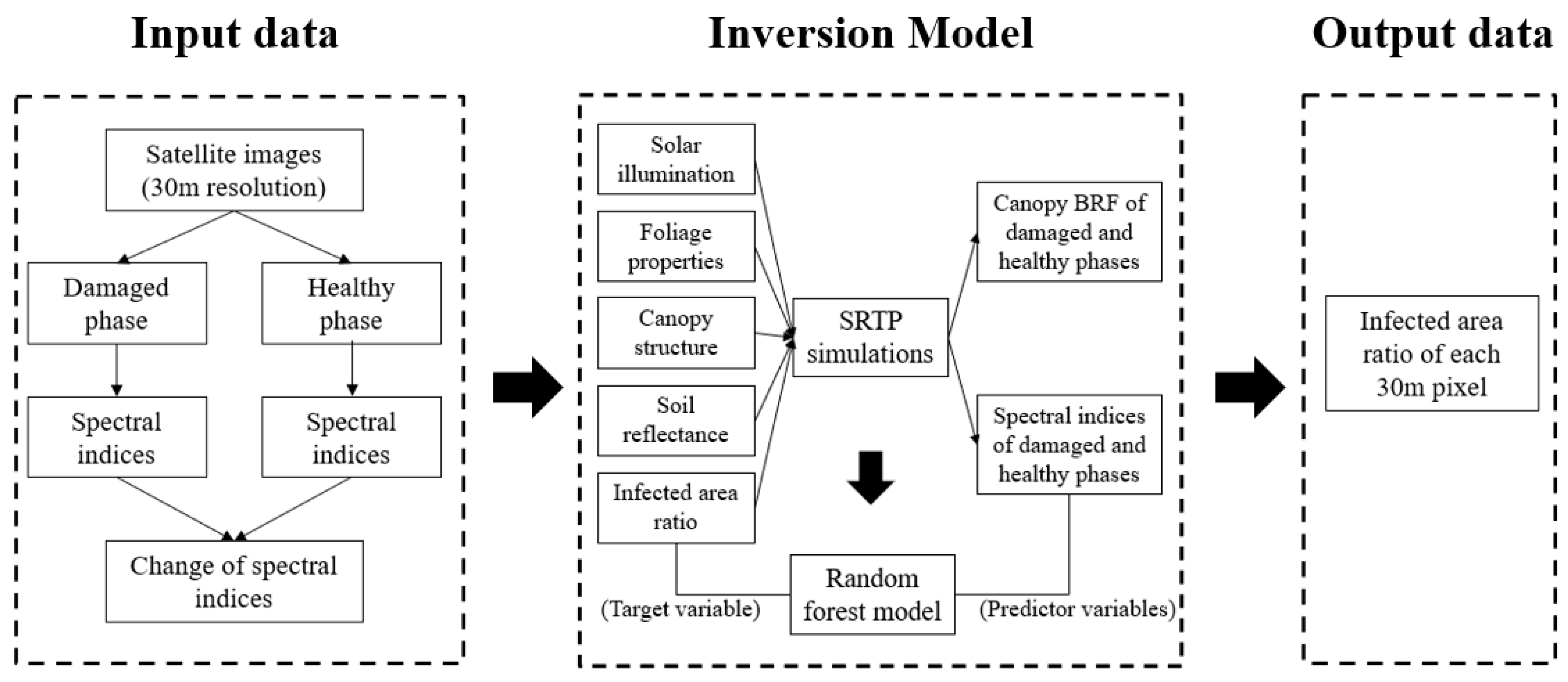
2.4. Parameter Inversion

In this study, we used the Infected Area Ratio (IAR) as the target parameter to be retrieved, which was defined as the ratio of the area of infected crowns to the plot area. IAR can be easily calculated by the model inputs, which is equal to the product of canopy coverage and yr.

2.4.1. The Random Forest

A random forest (RF) predictor [47] was utilized to build the model by the simulations of SRTP. Based on the scene simulations, the changes of 10 spectral indices were variables used to predict the target input IAR. Due to the discrimination ability of the predictor variables between the target values, the predictor variables can be sorted and ranked by the RF model [48]. In the RF algorithm, the variable importance is ranked by how much the “out-of-bag” (OOB) error of estimate increases when a single variable is excluded from the dataset. The result of OOB error indicates the mean decrease accuracy (MDA) of each variable, i.e., higher MDA means more importance of a variable [49]. We used MDA to assess the importance of the 10 spectral indices and employed the 10-fold cross-validation method for the robustness of the model established by the training dataset.

2.4.2. Inversion of IAR

The changes of the 10 spectral indices of two types of remote sensing images were calculated and input to the random forest model. The IAR of each plot was retrieved. The input/output data and the overall framework of the inversion model are shown in Figure 5. The LESS-extracted and UAV-measured data of infected areas were used to validate the model accuracy. The modeling and retrieving process was conducted in the Matlab toolbox “Random Forest”. The prediction accuracy was evaluated using the R2 and RMSE (Equations (2) and (3)).
R 2 = 1 i = 1 n ( y i y ^ i ) ² i = 1 n ( y i y ¯ ) ²
RMSE = i = 1 n ( y i y ^ i ) ² n
where n is the number of sample plots,   y i ^ is the predicted IAR, y i is the measured IAR, and y ¯ is the mean of measured IAR.

2.5. Comparative Experiments on the Inversion Model

In order to further evaluate the performance of the inversion model on field plots, two comparative experiments were conducted. First, to test the impact of background change on the inversion results, we repeated the process of modeling canopy reflectance of two phases by SRTP without considering the background change (i.e., the soil reflectance was fixed as the 30 samples in the healthy-stage image). The inversion without consideration of the background change was implemented for field plots as a comparison. Second, to analyze the advantages of using a physical model, we constructed a statistical RF model directly using the simulated plots as training samples, and tested the ability to invert infected areas in the Jiangxi and Shandong plots.

3. Results

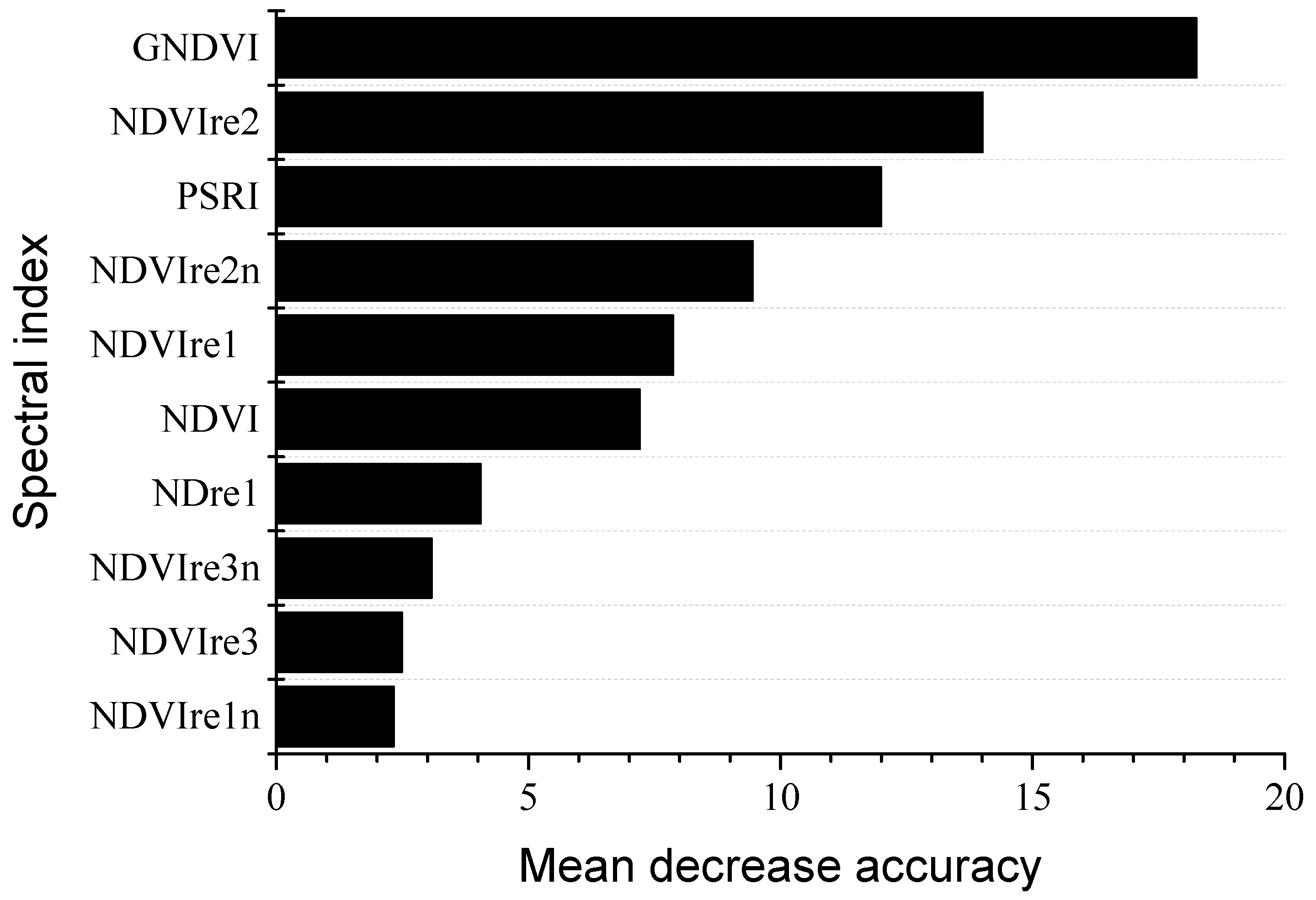
3.1. Importance of Spectral Indices

The variable importance of the 10 spectral indices of the RF model using MDA is shown in Figure 6. GNDVI suggests the most contribution to the IAR prediction, which is followed by NDVIre2 and PSRI. The rank of importance reveals the fact that the retrieving model was affected by the synergy of spectral indices established by green, red, red-edge and near-infrared bands.

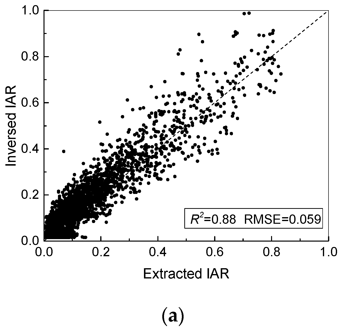
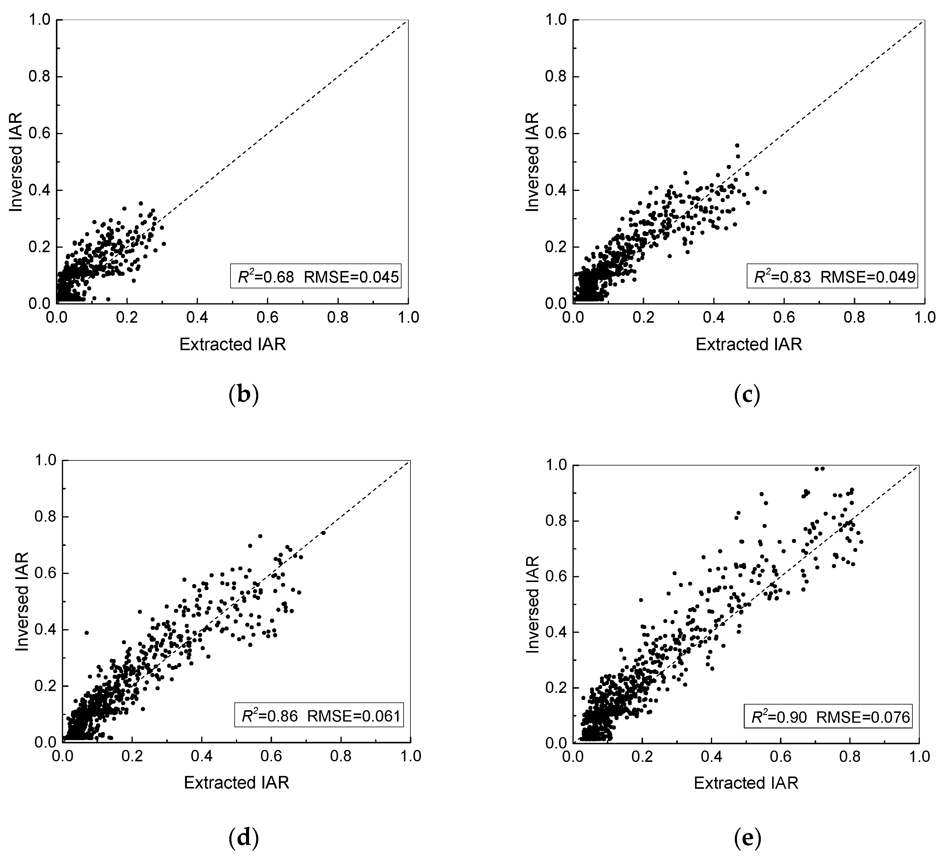
3.2. IAR Retrieval from the Simulated Images

The inversion results indicated good agreement with the extracted IAR values on the whole (Figure 7). The overall R2 between the retrieved values and the extracted values is 0.88. For the four plots of different damage level, R2 increases with damage probability while the RMSE is relatively stable for all the plots. The lowest R2 was achieved with the plots which contained only 25% damaged trees.

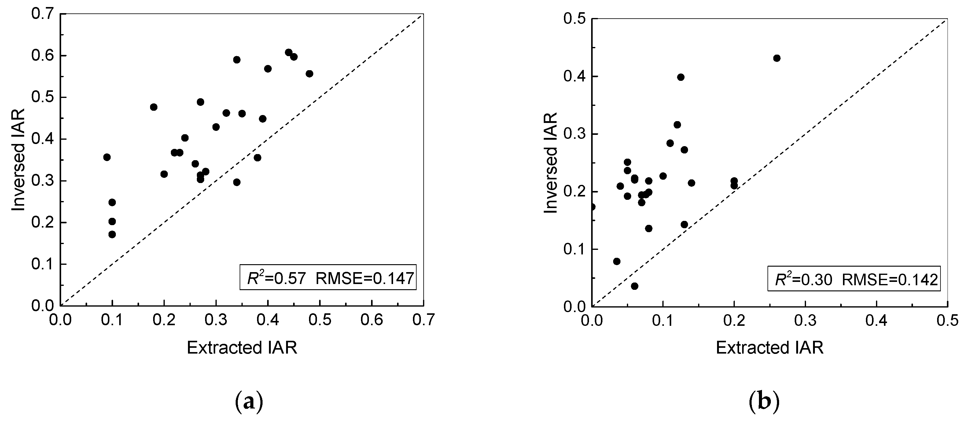
3.3. IAR Retrieval from the Sentinel-2 Images

The inversion results of Jiangxi and Shandong plots are shown in Figure 8. The R2 between the retrieved values and the extracted values are 0.57 and 0.48, respectively. The retrieval performance differs within the two study sites. Higher IAR values were retrieved as well as extracted for the Jiangxi plots than the Shandong plots (Figure 8).

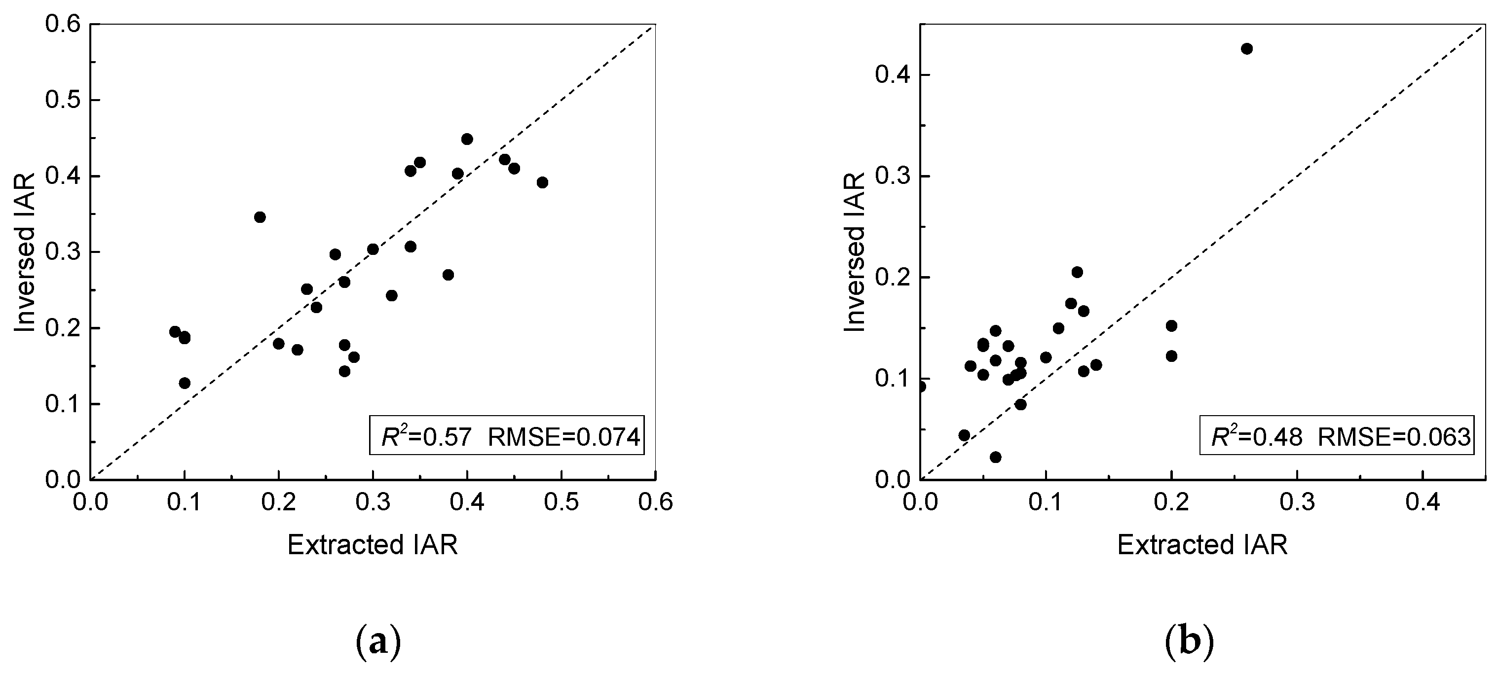
3.4. IAR Retrieval for the Comparative Experiment

The IAR retrieval results without consideration of the background change are shown in Figure 9. The results indicate that the infected area was overestimated for each case when not considering the background change. Figure 10 suggests the performance of the statistical RF model in the Jiangxi and Shandong plots. The inversion accuracy decreases in both study sites compared with the physically-based model.

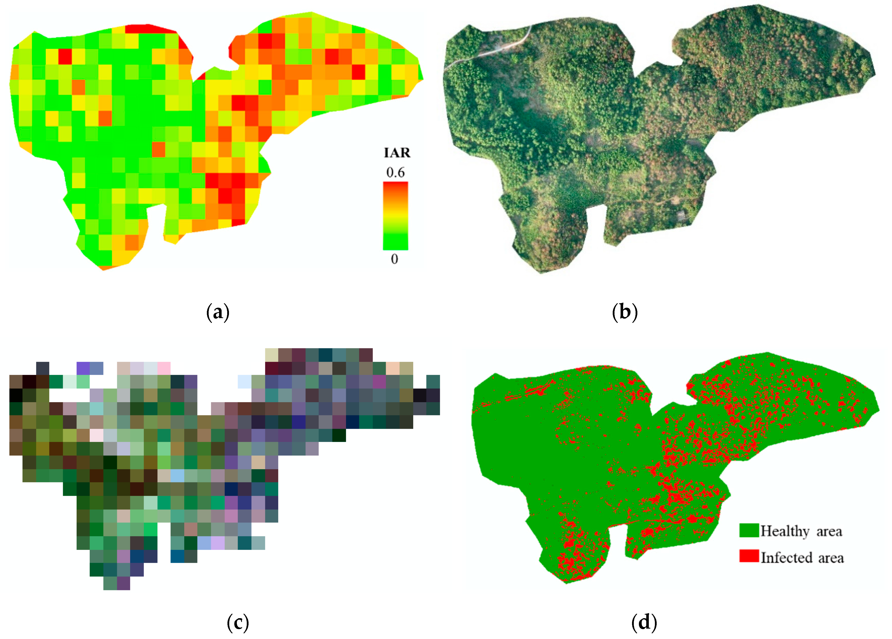
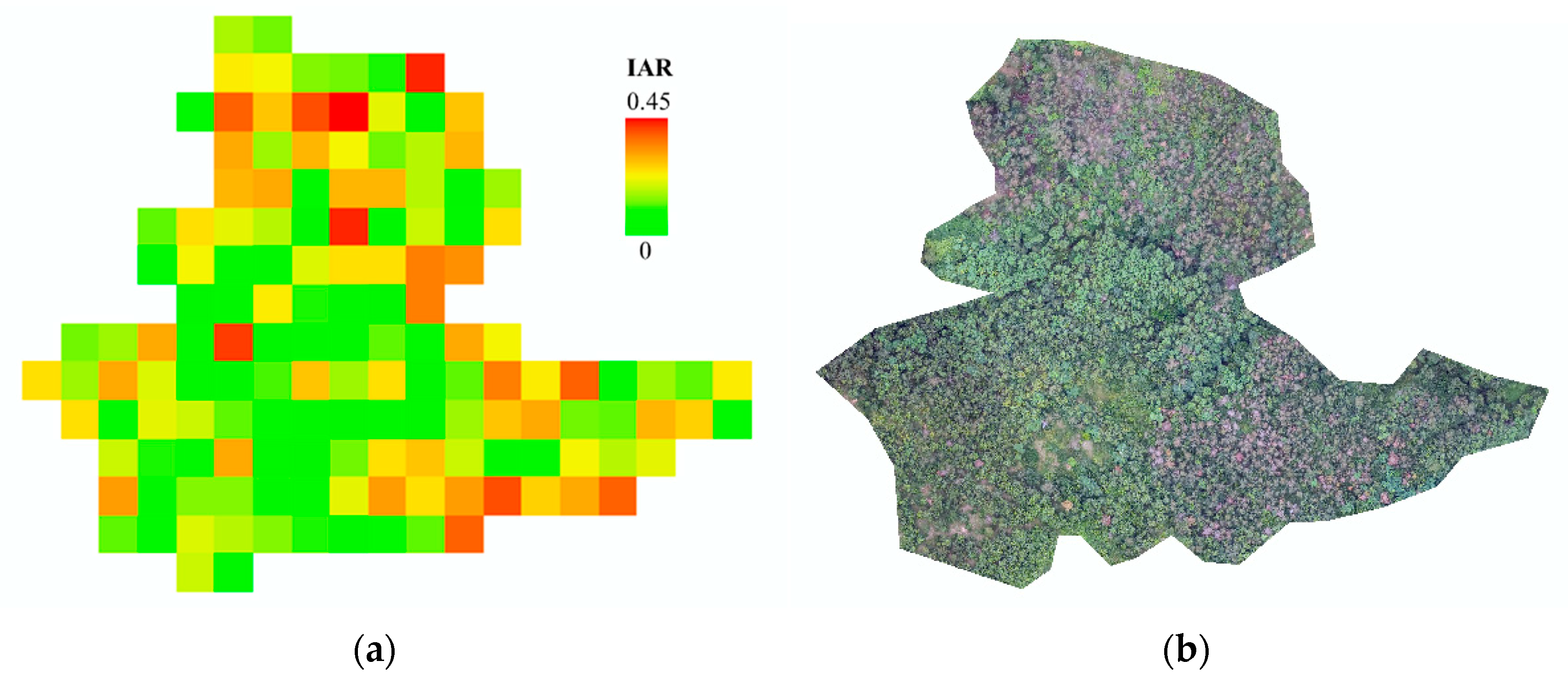
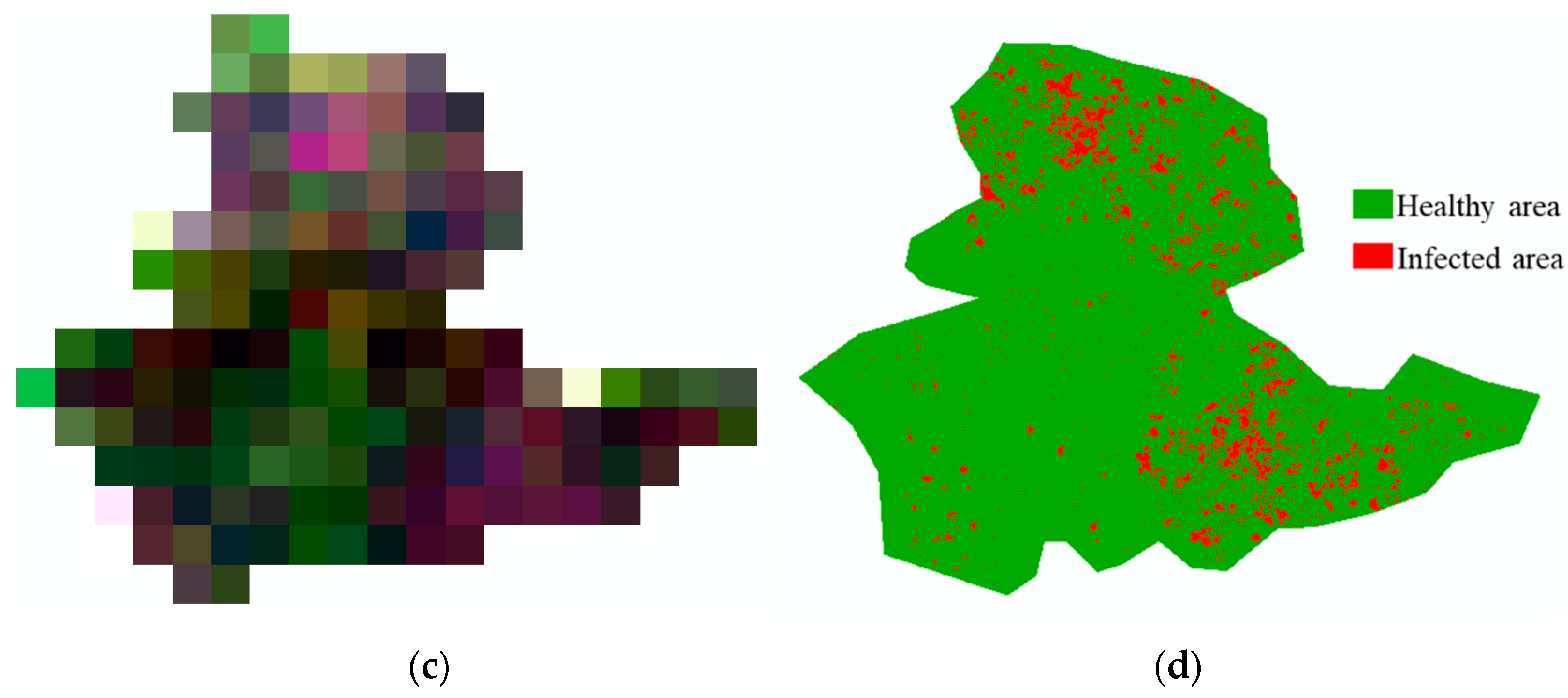
3.5. Infected Area Mapping

To extend to a large area, a pre-classification of pine forests from other land covers (e.g., farmlands, water bodies, buildings) is required. In this study, we extracted two representative pine forest regions based on the UAV images to map the infected areas. Figure 11a shows the inverted map of infected area in the Jiangxi forests, which is a region of masson pine trees with the size of about 35 hm2. Figure 12a displays the inverted map of infected area in the Shandong forests, which is an area of black pine trees with the size of about 15 hm2. The UAV RGB images and the Sentinel-2 RGB images at the same locations are displayed for comparison (Figure 11b,c and Figure 12b,c). To get the reference values of the infected area from the UAV images, Figure 11d and Figure 12d provide the supervised classification results by ENVI software, which consist of healthy areas and infected areas. The supervised classification was conducted by the maximum likelihood classification tool of ENVI, in which the training areas were selected by visual interpretation.
These two regions are typical, mainly composed of vegetation pixels, covering roads, bare land and large areas of pine forests. The result shows that the distribution of IAR obtained by inversion is in good agreement with the situation distinguished from the UAV image. The pixel discrimination of forests with high, medium and low IAR is good in general, and the healthy canopies mostly result in lower estimated values of IAR.

4. Discussion

4.1. Comparison of Inversion Performance for Different Damage Level

In the inversion application of RT models, the ill-posed problem always existed because the different combinations of parameters have compensation effects on canopy reflectance, leading to very similar solutions if using the simplified assumptions of the RT model [50,51]. The complicated scene factors can have complicated impacts on the accuracy of IAR inversion. Certain differences were observed among the inversion performance of the four simulated plots, which can be attributed to the variation of the damage level. The effects of damage level can be summarized as follows: (1) The inversion accuracy increased with yr. This can be explained by the ratio change between infected area and background area, which are the two main causes of the signal change. When yr is low, the background change contributes more to the remote sensing signal, which interferes the inversion accuracy of infected areas. Such an effect is weakened at higher damage level as the contribution of infected area increases. (2) A slight underestimation at high infected area was observed when yr = 1. Such bias may not be simply caused by estimation error, but rather be affected by the inaccurate values of the extracted infected area. When the infected area is high, crowns may block each other. The intersection area cannot be well distinguished, leading to overestimation of the extracted infected area, which explains the observed underestimation of the infected area.

4.2. The Impact of Study Sites on Inversion Performance

In this study, the inversion model was tested by three sites: the LESS-simulated plots, Jiangxi plots and Shandong plots. The inversion approach performed well on the whole but was also impacted by different study sites. For the simulated plots, the model showed the highest accuracy (R2 = 0.88, RMSE = 0.059). The real plots indicated lower accuracy than the simulated plots due to the complexity of forest scenes. Although the simulated plots were generated according to the prior knowledge of real forests, the complicated heterogeneity of canopy structure, damage degree and soil background cannot be perfectly defined. There are four sources of error in real plots. First, there are differences in the structure of tree crowns in the scene, and the simplification idea of the model will affect the inversion accuracy. Second, the damage degree of damaged trees is not exactly the same, and there are differences in chlorophyll and other contents among trees, which is difficult to quantify for incompletely damaged trees. Third, the spectral heterogeneity of soil background is large, and it is difficult to fully evaluate the change degree in healthy period and damaged period. Fourth, there may be some deviation in the reference value of the infected area extracted from the UAV sample plots.
The inversion performance also differed between Jiangxi and Shandong plots. The accuracy of Jiangxi plots was higher than that of Shandong plots. This result can be attributed to the difference of forest properties. In Jiangxi plots, the canopies were dense in which patches of crowns were infected; while in Shandong plots, isolated individual trees were distributed within the sparse canopies. The error of canopies with lower yr is consistent with the performance of the simulated plots. Moreover, a precise disease assessment requires a quantitative estimation of the temporal evolution of the disease [32]. The damage stage of Shandong plots was not uniform, resulting in difficulty assessing the precise area of the infected trees.
The results of each site indicate the applicability of the approaches in different forest types and study sites. Although only two regions of real forests were used for ground validation, the interregional variations were found to be feasible through physically-based simulations of different forest scenarios. Theoretically, the model can be used in more study sites if done with proper adjustment of the scenario simulations with input parameters from wider field knowledge.

4.3. Consideration of the Background Change

Consideration of canopy heterogeneity is a promising way to improve retrieval performance of RT models [6]. In this approach, the objective of using images of two phases was to zoom in on the changes between them. The phenological change of healthy trees was neglected because it is weaker for evergreen conifers than broadleaf species. However, the background change may be strong especially in sparse canopies. In this study, we considered the background change in the process of modeling the canopy reflectance of two phases by SRT and conducted a comparative experiment without considering the background change. The results of the two models indicate that infected areas may be overestimated for each case when not considering the background change. This can be explained by the fact that the defoliation of the forest understory has an impact on the canopy reflectance, which may be an interference in identifying the infection of tree crowns. The inversion approach with consideration of the background change can increase the inversion accuracy.

4.4. The Use of Physical Model Comparing to Regression

Compared with traditional statistical regression approaches, the purpose of using a physical model was to improve the versatility of the inversion model in different regions. The result of the comparative experiment by the statistical RF model indicates that traditional statistical regression is more dependent on the local training samples. It is hardly scalable among different study sites, regardless of the regional variation of forests. The local over fitting of statistical models existed in most previous studies on PWD monitoring [52,53]. Therefore, it is feasible to use one RF model in a specific study site, but a new model is needed when studying in another region.
For the future application of large-scaled PWD monitoring, it might be not feasible to obtain enough training samples. The approach in this study provides a new idea to map the infected area of PWD, in which only small amount of prior knowledge is needed. With the acquisition of pine forest regions, large-scaled production of PWD infection area will be studied in the future.

4.5. The Drawbacks and Future Work

The limitations of this study include three aspects that need to be considered in future work. (1) The test data of this study are mainly simulated plots. In the simulated plots, a variety of possible canopies infected by PWD were considered to test the inversion approach. However, only 25 in each of the two study sites are selected for real plots. More study regions need to be tested in the future to examine the performance for more scenarios. (2) To simplify the forest structure, tree crowns were assumed simply as cylinders and the spatial aggregation effect of the damaged trees was not considered in the current study. The uncertainty caused by this assumption was evaluated in our previous study [33]. As the mixed patterns of healthy and damaged trees in the real forests are spatially complex and varying with time, such simplifications can improve computing efficiency without losing too much accuracy. In the situation in which damaged trees are regularly clustered, the simulation accuracy may be further increased if we modify the inputted pair–correlation function based on the simulation of Matérn cluster process. (3) In our study, we tried to propose a simple inversion method for large-scale detection of PWD without too much prior knowledge. The balance of accuracy and simplification should be considered according to the practical application. To further increase the accuracy, the ill-posed inversion problem can be alleviated with some regularization methods. The saturation problem of BRF in optical remote sensing can be alleviated by the involvement of multi-angular information; more realistic canopy structures can be retrieved from lidar data. (4) This study focused on the pine forests infected by PWD because such a disease is a main disturbance in many pine forest regions. When the forest disturbance is mixed with other stresses (e.g., other pests and drought), the detection accuracy of PWD area may be affected. Nevertheless, SRTP provides a theoretical framework for different kinds of disturbances by adjusting the input optical and structural parameters of stressed foliage. The variations among different disturbances may be studied in a future work.

5. Conclusions

This study explored the application of the extended SRTP model in the quantitative inversion of an infection area of forest PWD. In this approach, model simulations by SRTP based on a small amount of prior knowledge were coupled with a random forest algorithm. The infected area of PWD was retrieved from medium resolution remote sensing images, which were tested by the 3D model simulated sample plots and the PWD-stressed forest sample plots in Jiangxi and Shandong. The inversion method performs best in the three-dimensional model LESS simulation sample plot (R2 = 0.88, RMSE = 0.059), and the inversion accuracy decreases in the real forest sample plot, but it still has certain application value. The inversion accuracy is different for Jiangxi masson pine stand with large coverage and serious damage (R2 = 0.57, RMSE = 0.074), and for Shandong black pine stand with sparse and a small number of single plant damage (R2 = 0.48, RMSE = 0.063). This study indicates that the SRTP model is a feasible and simple tool for pest damage inversion at large scale. The stochastic radiative transfer theory provides a potential approach for future monitoring of terrestrial vegetation parameters.

Author Contributions

Conceptualization, X.L. and H.H.; methodology, X.L.; software, T.T., T.L. and L.L.; validation, Y.R.; formal analysis, X.L., T.T. and T.L.; investigation, J.W. and D.W.; writing—original draft preparation, X.L.; writing—review and editing, X.L. and H.H.; visualization, D.J.; supervision, H.H. All authors have read and agreed to the published version of the manuscript.

Funding

This paper has been supported by Major emergency science and technology project of National Forestry and Grassland Administration, China (ZD202001); and Beijing’s Science and Technology Planning Project, China (Z201100008020001).

Institutional Review Board Statement

Not applicable.

Informed Consent Statement

Not applicable.

Acknowledgments

The authors would like to thank Nikolay Shabanov for the fruitful discussions on SRTP modeling. The authors thank Shengwang Meng, Xu Zhao, Pengfei Guo, Zhexiu Yu and Kunjian Wen for the field measurements in 2019 and 2021.

Conflicts of Interest

The authors declare that they have no known competing financial interests or personal relationships that could have appeared to influence the work reported in this paper.

References

  1. Ikegami, M.; Jenkins, T.A.R. Estimate global risks of a forest disease under current and future climates using species distribution model and simple thermal model Pine Wilt disease as a model case. For. Ecol. Manag. 2018, 409, 343–352. [Google Scholar] [CrossRef]
  2. Ye, J. Epidemic Status of Pine Wilt Disease in China and Its Prevention and Control Techniques and Counter Measures. Sci. Silvae Sin. 2019, 55, 1–10. [Google Scholar] [CrossRef]
  3. Ichihara, Y.; Fukuda, K.; Suzuki, K. Early Symptom Development and Histological Changes Associated with Migration of Bursaphelenchus xylophilus in Seedling Tissues of Pinus thunbergii. Plant Dis. 2000, 84, 675–680. [Google Scholar] [CrossRef] [PubMed] [Green Version]
  4. Sun, H.; Zhou, Y.; Li, X.; Zhang, Y.; Wang, Y. Occurrence of major forest pests in 2020 and prediction of occurrence trend in 2021 in China. For. Pest Dis. 2021, 40, 45–48. [Google Scholar]
  5. Yu, R.; Luo, Y.; Zhou, Q.; Zhang, X.; Ren, L. A machine learning algorithm to detect pine wilt disease using UAV-based hyperspectral imagery and LiDAR data at the tree level. Int. J. Appl. Earth Obs. Geoinf. 2021, 101, 102363. [Google Scholar] [CrossRef]
  6. Lin, Q.; Huang, H.; Wang, J.; Huang, K.; Liu, Y. Detection of Pine Shoot Beetle (PSB) Stress on Pine Forests at Individual Tree Level using UAV-Based Hyperspectral Imagery and Lidar. Remote Sens. 2019, 11, 2540. [Google Scholar] [CrossRef] [Green Version]
  7. Franklin, S.E.; Wulder, M.A.; Skakun, R.S.; Carroll, A.L. Mountain pine beetle red-attack forest damage classification using stratified Landsat TM data in British Columbia, Canada. Photogramm. Eng. Remote Sens. 2003, 69, 283–288. [Google Scholar] [CrossRef]
  8. Hicke, J.A.; Logan, J. Mapping whitebark pine mortality caused by a mountain pine beetle outbreak with high spatial resolution satellite imagery. Int. J. Remote Sens. 2009, 30, 4427–4441. [Google Scholar] [CrossRef]
  9. Kim, S.R.; Lee, W.K.; Lim, C.H.; Kim, M.; Kafatos, M.C.; Lee, S.H.; Lee, S.S. Hyperspectral Analysis of Pine Wilt Disease to Determine an Optimal Detection Index. Forests 2018, 9, 115. [Google Scholar] [CrossRef] [Green Version]
  10. Chen, G.; Meentemeyer, R.K. Remote Sensing of Forest Damage by Diseases and Insects. In Remote Sensing for Sustainability; CRC Press: Boca Raton, FL, USA, 2016; pp. 145–162. [Google Scholar]
  11. Coops, N.C.; Johnson, M.; Wulder, M.A.; White, J.C. Assessment of QuickBird high spatial resolution imagery to detect red attack damage due to mountain pine beetle infestation. Remote Sens. Environ. 2006, 103, 67–80. [Google Scholar] [CrossRef]
  12. Olsson, P.O.; Jonsson, A.M.; Eklundh, L. A new invasive insect in Sweden-Physokermes inopinatus: Tracing forest damage with satellite based remote sensing. For. Ecol. Manag. 2012, 285, 29–37. [Google Scholar] [CrossRef]
  13. Coops, N.C.; Gillanders, S.N.; Wulder, M.A.; Gergel, S.E.; Nelson, T.; Goodwin, N.R. Assessing changes in forest fragmentation following infestation using time series Landsat imagery. For. Ecol. Manag. 2010, 259, 2355–2365. [Google Scholar] [CrossRef]
  14. Goodwin, N.R.; Coops, N.C.; Wulder, M.A.; Gillanders, S.; Schroeder, T.A.; Nelson, T. Estimation of insect infestation dynamics using a temporal sequence of Landsat data. Remote Sens. Environ. 2008, 112, 3680–3689. [Google Scholar] [CrossRef]
  15. Coops, N.C.; Wulder, M.A.; Iwanicka, D. Large area monitoring with a MODIS-based Disturbance Index (DI) sensitive to annual and seasonal variations. Remote Sens. Environ. 2009, 113, 1250–1261. [Google Scholar] [CrossRef]
  16. Skakun, R.S.; Wulder, M.A.; Franklin, S.E. Sensitivity of the thematic mapper enhanced wetness difference index to detect mountain pine beetle red-attack damage. Remote Sens. Environ. 2003, 86, 433–443. [Google Scholar] [CrossRef]
  17. Adelabu, S.; Mutanga, O.; Adam, E. Evaluating the impact of red-edge band from Rapideye image for classifying insect defoliation levels. ISPRS J. Photogramm. Remote Sens. 2014, 95, 34–41. [Google Scholar] [CrossRef]
  18. Bright, B.C.; Hicke, J.A.; Hudak, A.T. Estimating aboveground carbon stocks of a forest affected by mountain pine beetle in Idaho using lidar and multispectral imagery. Remote Sens. Environ. 2012, 124, 270–281. [Google Scholar] [CrossRef] [Green Version]
  19. Meddens, A.J.H.; Hicke, J.A.; Vierling, L.A. Evaluating the potential of multispectral imagery to map multiple stages of tree mortality. Remote Sens. Environ. 2011, 115, 1632–1642. [Google Scholar] [CrossRef]
  20. Thayn, J.B. Using a remotely sensed optimized Disturbance Index to detect insect defoliation in the Apostle Islands, Wisconsin, USA. Remote Sens. Environ. 2013, 136, 210–217. [Google Scholar] [CrossRef]
  21. Walter, J.A.; Platt, R.V. Multi-temporal analysis reveals that predictors of mountain pine beetle infestation change during outbreak cycles. For. Ecol. Manag. 2013, 302, 308–318. [Google Scholar] [CrossRef]
  22. Cheng, T.; Rivard, B.; Sanchez-Azofeifa, G.A.; Feng, J.; Calvo-Polanco, M. Continuous wavelet analysis for the detection of green attack damage due to mountain pine beetle infestation. Remote Sens. Environ. 2010, 114, 899–910. [Google Scholar] [CrossRef]
  23. Oumar, Z.; Mutanga, O. Integrating environmental variables and WorldView-2 image data to improve the prediction and mapping of Thaumastocoris peregrinus (bronze bug) damage in plantation forests. ISPRS J. Photogramm. Remote Sens. 2014, 87, 39–46. [Google Scholar] [CrossRef]
  24. Oumar, Z.; Mutanga, O.; Ismail, R. Predicting Thaumastocoris peregrinus damage using narrow band normalized indices and hyperspectral indices using field spectra resampled to the Hyperion sensor. Int. J. Appl. Earth Obs. Geoinf. 2013, 21, 113–121. [Google Scholar] [CrossRef]
  25. Pontius, J.; Martin, M.; Plourde, L.; Hallett, R. Ash decline assessment in emerald ash borer-infested regions: A test of tree-level, hyperspectral technologies. Remote Sens. Environ. 2008, 112, 2665–2676. [Google Scholar] [CrossRef]
  26. Babst, F.; Esper, J.; Parlow, E. Landsat TM/ETM plus and tree-ring based assessment of spatiotemporal patterns of the autumnal moth (Epirrita autumnata) in northernmost Fennoscandia. Remote Sens. Environ. 2010, 114, 637–646. [Google Scholar] [CrossRef]
  27. Kennedy, R.E.; Yang, Z.G.; Cohen, W.B. Detecting trends in forest disturbance and recovery using yearly Landsat time series: 1. LandTrendr-Temporal segmentation algorithms. Remote Sens. Environ. 2010, 114, 2897–2910. [Google Scholar] [CrossRef]
  28. Meigs, G.W.; Kennedy, R.E.; Cohen, W.B. A Landsat time series approach to characterize bark beetle and defoliator impacts on tree mortality and surface fuels in conifer forests. Remote Sens. Environ. 2011, 115, 3707–3718. [Google Scholar] [CrossRef]
  29. Townsend, P.A.; Singh, A.; Foster, J.R.; Rehberg, N.J.; Kingdon, C.C.; Eshleman, K.N.; Seagle, S.W. A general Landsat model to predict canopy defoliation in broadleaf deciduous forests. Remote Sens. Environ. 2012, 119, 255–265. [Google Scholar] [CrossRef]
  30. Lin, Q.; Huang, H.; Yu, L.; Wang, J. Detection of shoot beetle stress on yunnan pine forest using a coupled LIBERTY2-INFORM simulation. Remote Sens. 2018, 10, 1133. [Google Scholar] [CrossRef] [Green Version]
  31. Lin, Q.; Huang, H.; Chen, L.; Wang, J.; Liu, Y. Using the 3D model RAPID to invert the shoot dieback ratio of vertically heterogeneous Yunnan pine forests to detect beetle damage. Remote Sens. Environ. 2021, 260, 112475. [Google Scholar] [CrossRef]
  32. Hornero, A.; Hernández-Clemente, R.; North, P.R.J.; Beck, P.S.A.; Boscia, D.; Navas-Cortes, J.A.; Zarco-Tejada, P.J. Monitoring the incidence of Xylella fastidiosa infection in olive orchards using ground-based evaluations, airborne imaging spectroscopy and Sentinel-2 time series through 3-D radiative transfer modelling. Remote Sens. Environ. 2020, 236, 111480. [Google Scholar] [CrossRef]
  33. Li, X.; Huang, H.; Shabanov, N.V.; Chen, L.; Yan, K.; Shi, J. Extending the stochastic radiative transfer theory to simulate BRF over forests with heterogeneous distribution of damaged foliage inside of tree crowns. Remote Sens. Environ. 2020, 250, 112040. [Google Scholar] [CrossRef]
  34. Huang, H.G.; Qin, W.H.; Liu, Q.H. RAPID: A Radiosity Applicable to Porous IndiviDual Objects for directional reflectance over complex vegetated scenes. Remote Sens. Environ. 2013, 132, 221–237. [Google Scholar] [CrossRef]
  35. Qi, J.B.; Xie, D.H.; Yin, T.G.; Yan, G.J.; Gastellu-Etchegorry, J.P.; Li, L.Y.; Zhang, W.M.; Mu, X.H.; Norford, L.K. LESS: LargE-Scale remote sensing data and image simulation framework over heterogeneous 3D scenes. Remote Sens. Environ. 2019, 221, 695–706. [Google Scholar] [CrossRef]
  36. Defries, R.S.; Townshend, J.R.G. NDVI-derived land cover classifications at a global scale. Int. J. Remote Sens. 1994, 15, 3567–3586. [Google Scholar] [CrossRef]
  37. Gitelson, A.A.; Kaufman, Y.J.; Merzlyak, M.N. Use of a green channel in remote sensing of global vegetation from EOS-MODIS. Remote Sens. Environ. 1996, 58, 289–298. [Google Scholar] [CrossRef]
  38. Merzlyak, M.N.; Chivkunova, O.B.; Gitelson, A.A.; Rakitin, V.Y. Non-destructive optical detection of pigment changes during leaf senescence and fruit ripening. Physiol. Plant. 2010, 106, 135–141. [Google Scholar] [CrossRef] [Green Version]
  39. Gitelson, A.A.; Merzlyak, M.N. Spectral Reflectance Changes Associated with Autumn Senescence of Aesculus hippocastanum L. and Acer platanoides L. Leaves. Spectral Features and Relation to Chlorophyll Estimation. J. Plant Physiol. 1994, 143, 286–292. [Google Scholar] [CrossRef]
  40. Fernández-Manso, A.; Fernández-Manso, O.; Quintano, C. SENTINEL-2A red-edge spectral indices suitability for discriminating burn severity. Int. J. Appl. Earth Obs. Geoinf. 2016, 50, 170–175. [Google Scholar] [CrossRef]
  41. Sims, D.A.; Gamon, J.A. Relationships between leaf pigment content and spectral reflectance across a wide range of species, leaf structures and developmental stages. Remote Sens. Environ. 2002, 81, 337–354. [Google Scholar] [CrossRef]
  42. Ross, J. The Radiation Regime and Architecture of Plant Stands; Dr. W. Junk: Norwell, MA, USA, 1981; p. 391. [Google Scholar]
  43. Knyazikhin, Y.; Kranigk, J.; Myneni, R.B.; Panfyorov, O.; Gravenhorst, G. Influence of small-scale structure on radiative transfer and photosynthesis in vegetation cover. J. Geophys. Res. Atmos. 1998, 103, 6133–6144. [Google Scholar] [CrossRef]
  44. Shabanov, N.V.; Knyazikhin, Y.; Baret, F.; Myneni, R.B. Stochastic Modeling of Radiation Regime in Discontinuous Vegetation Canopies. Remote Sens. Environ. 2000, 74, 125–144. [Google Scholar] [CrossRef]
  45. Shabanov, N.V.; Huang, D.; Knjazikhin, Y.; Dickinson, R.E.; Myneni, R.B. Stochastic radiative transfer model for mixture of discontinuous vegetation canopies. J. Quant. Spectrosc. Radiat. Transf. 2007, 107, 236–262. [Google Scholar] [CrossRef] [Green Version]
  46. Stoyan, D.; Kendall, W.S.; Mecke, J. Stochastic Geometry and its Applications. J. R. Stat. Soc. 2013, 45, 345. [Google Scholar]
  47. Breiman, L. Random Forests. Mach. Learn. 2001, 45, 5–32. [Google Scholar] [CrossRef] [Green Version]
  48. Belgiu, M.; Drăguţ, L. Random forest in remote sensing: A review of applications and future directions. ISPRS J. Photogramm. Remote Sens. 2016, 114, 24–31. [Google Scholar] [CrossRef]
  49. Immitzer, M.; Atzberger, C.; Koukal, T. Tree Species Classification with Random Forest Using Very High Spatial Resolution 8-Band WorldView-2 Satellite Data. Remote Sens. 2012, 4, 2661–2693. [Google Scholar] [CrossRef] [Green Version]
  50. Rivera, J.P.; Verrelst, J.; Leonenko, G.; Moreno, J. Multiple Cost Functions and Regularization Options for Improved Retrieval of Leaf Chlorophyll Content and LAI through Inversion of the PROSAIL Model. Remote Sens. 2013, 5, 3280–3304. [Google Scholar] [CrossRef] [Green Version]
  51. Verrelst, J.; Rivera, J.P.; Leonenko, G.; Alonso, L.; Moreno, J. Optimizing LUT-Based RTM Inversion for Semiautomatic Mapping of Crop Biophysical Parameters from Sentinel-2 and-3 Data: Role of Cost Functions. IEEE Trans. Geosci. Remote Sens. 2014, 52, 257–269. [Google Scholar] [CrossRef]
  52. Higashi, T. Extraction of Expanded Area of Damaged Stands by Pine Wilt Disease Using Two Landsat TM Data. J. Remote Sens. Soc. Jpn. 2009, 10, 389–395. [Google Scholar]
  53. Syifa, M.; Park, S.J.; Lee, C.W. Detection of the Pine Wilt Disease Tree Candidates for Drone Remote Sensing Using Artificial Intelligence Techniques. Engineering 2020, 6, 919–926. [Google Scholar] [CrossRef]
Figure 1. The location of study area and the field sample plots. The dot and triangle represent Jiangxi sample plot and Shandong sample plot, respectively.
Remotesensing 14 01526 g001
Figure 2. The reflectance and transmittance of healthy and damaged needles of masson pine and black pine.
Remotesensing 14 01526 g002
Figure 3. The individual tree and the 900 m × 900 m plot generated by LESS. (a) The obj-file of the individual tree. (b) The 900 m × 900 m plot, in which the round dots denote trees. The orange line and the green line represent the directions of the sun and the sensor, respectively. The tree stem density decreases from left (796/hm2) to right (79.6/hm2).
Remotesensing 14 01526 g003
Figure 4. The field plots established from the UAV images. (a,c) Masson pine plots in Jiangxi. (b,d) Black pine plots in Shandong. (a,b) Indicate the infected stage, while (c,d) indicate the corresponding healthy stage.
Remotesensing 14 01526 g004
Figure 5. The input/output data and the overall framework of the inversion model.
Remotesensing 14 01526 g005
Figure 6. The variable importance of the 10 spectral indices in the RF model.
Remotesensing 14 01526 g006
Figure 7. The results of IAR retrieval from the simulated images. (a) The results of all the four plots. (be) indicate each of the four plots in which the random probabilities of generating damaged trees are 0.25, 0.5, 0.75 and 1, respectively.
Remotesensing 14 01526 g007aRemotesensing 14 01526 g007b
Figure 8. The results of IAR retrieval of Jiangxi and Shandong plots. (a) Masson pine plots in Jiangxi. (b) Black pine plots in Shandong.
Remotesensing 14 01526 g008
Figure 9. The results of IAR retrieval of Jiangxi and Shandong plots without consideration of the background change. (a) Masson pine plots in Jiangxi. (b) Black pine plots in Shandong.
Remotesensing 14 01526 g009
Figure 10. The results of IAR retrieval of Jiangxi and Shandong plots by statistical RF model. (a) Masson pine plots in Jiangxi. (b) Black pine plots in Shandong.
Remotesensing 14 01526 g010
Figure 11. Infected area map of typical region of masson pine trees. (a) The 30 m-resolution IAR map. (b) The corresponding UAV RGB image. (c) The corresponding Sentinel-2 RGB image. (d) The reference classification results from the UAV image.
Remotesensing 14 01526 g011
Figure 12. Infected area map of typical region of black pine trees. (a) The 30 m-resolution IAR map. (b) The corresponding UAV RGB image. (c) The corresponding Sentinel-2 RGB image. (d) The reference classification results from the UAV image.
Remotesensing 14 01526 g012aRemotesensing 14 01526 g012b
Table 1. The equations of 10 vegetation spectral indices.
Spectral IndexEquationReference
NDVI(B8 − B4)/(B8 + B4)[36]
GNDVI(B8 − B3)/(B8 + B3)[37]
PSRI(B4 − B3)/B6[38]
NDVIre1(B8 − B5)/(B8 + B5)[39]
NDVIre1n(B8a − B5)/(B8a + B5)[40]
NDVIre2(B8 − B6)/(B8 + B6)[39]
NDVIre2n(B8a − B6)/(B8a + B6)[40]
NDVIre3(B8 − B7)/(B8 + B7)[39]
NDVIre3n(B8a − B7)/(B8a + B7)[40]
NDre1(B6 − B5)/(B6 + B5)[41]
Table 2. The setting of input variables in SRTP simulations of infected scenarios.
VariableSetting RangeStep
Canopy coverage[0.05, 0.95]0.05
Leaf area volume density (m2 m−3)[2, 6]0.5
Ratio of amount of infected trees to total amount of trees[0, 1]0.05
Aspect ratio1.67
Leaf angle distributionSpherical
Publisher’s Note: MDPI stays neutral with regard to jurisdictional claims in published maps and institutional affiliations.

