
Evaluation and Global-Scale Observation of Nitrous Oxide from IASI on Metop-A
by
 , , ,
, , ,
Rémi Chalinel
1, 
Jean-Luc Attié
1,*,
Philippe Ricaud
2,
Jérôme Vidot
3,
Yannick Kangah
4,
Didier Hauglustaine
5 and
Rona Thompson
6 1
LAERO-Laboratoire d’Aérologie, Université de Toulouse, UPS, CNRS, 14 Avenue Edouard Belin, 31400 Toulouse, France
2
CNRM-Centre National de Recherches Météorologiques, Université de Toulouse, Météo-France, CNRS, 42 Avenue Gaspard Coriolis, CEDEX, 31057 Toulouse, France
3
CEMS-Centre d’Études en Météorologie Satellitaire, CNRM, Météo-France, CNRS, Avenue de Lorraine, CEDEX, 22307 Lannion, France
4
SPASCIA-Space Science Algorithmics, Parc Technologique du Canal, 14 Avenue de l’Europe, 31520 Ramonville Saint Agne, France
5
LSCE-Laboratoire des Sciences du Climat et de l’Environnement, Institut Pierre-Simon Laplace, CEA Saclay, Orme des Merisiers, 91191 Gif-sur-Yvette, France
6
NILU-Norsk Institutt for Luftforskning, Instituttveien 18, 2007 Kjeller, Norway
*
Author to whom correspondence should be addressed.
Remote Sens. 2022, 14(6), 1403; https://doi.org/10.3390/rs14061403
Submission received: 27 January 2022
/
Revised: 25 February 2022
/
Accepted: 4 March 2022
/
Published: 14 March 2022
(This article belongs to the Special Issue Advances in Infrared Observation of Earth's Atmosphere)
Abstract
:Nitrous oxide (NO) is a greenhouse gas difficult to estimate by satellite because of its weak spectral signature in the infra-red band and its low variability in the troposphere. Nevertheless, this study presents the evaluation of new tropospheric NO observations from the Infrared Atmospheric Sounder Interferometer (IASI) on Metop-A using the Toulouse NO Retrieval Version 2.0 tool. This tool is based on the Radiative Transfer for Tiros Operational Vertical sounder (RTTOV) model version 12.3 coupled to the Levenberg-Marquardt optimal estimation method enabling the simultaneous retrieval of methane, water vapour, temperature profiles together with surface temperature and emissivity within the 1240–1350 cm window. In this study, we focused on the upper troposphere (300 hPa) where the sensitivity of IASI is significant. The IASI NO data has been evaluated using aircraft NO observations from the High-performance Instrumented Airborne Platform for Environmental Research Pole-to-Pole Observations (HIPPO) campaigns in 2009, 2010, and 2011 and from the National Oceanic and Atmospheric Administration’s (NOAA) Global Greenhouse Gas Reference Network (GGGRN) in 2011. In addition, we evaluated the IASI NO using ground-based NO measurements from 9 stations belonging to the Network for the Detection of Atmospheric Composition Change (NDACC). We found a total random error of ∼2 ppbv (0.6%) for one single retrieval at 300 hPa. Under favorable conditions, this error is also found in the vertical level pressure range 300–500 hPa. It decreases rapidly to ∼0.4 ppbv (0.1%) when we average on a 1° × 1° box. In addition, independent observations allows the estimation of bias with the IASI TNOR v2.0 NO. The bias between IASI and aircraft NO data at 300 hPa is ∼1.0 ppbv (∼0.3%). We found an estimated random error of ∼2.3 ppbv (∼0.75%). This study also shows relatively high correlations between IASI data and aircraft in situ profiles but more varying correlations over the year 2011 depending on the location between IASI and NDACC remote sensing data. Finally, we present daily, monthly, and seasonal IASI NO horizontal distributions in the upper troposphere as well as cross sections for different seasons that exhibit maxima in the Tropical band especially over Africa and South America.
Keywords:
nitrous oxide; space-borne observations; validation; IASI; HIPPO; NDACC; NOAA airborne observations1. Introduction
After water vapor (HO), carbon dioxide (CO) and methane (CH), nitrous oxide (NO), with a lifetime of 116 years [1], is the most important greenhouse gas (GHG) contributing to global warming [2]. It has a global warming potential 296 times higher than that of CO on a mass basis over a 100-year horizon. Consequently, NO has a radiative forcing that is equivalent to ∼10% that of CO, although it is 1000 times less abundant. Furthermore, emissions of NO are currently the most important emissions with respect to stratospheric ozone depletion and are impeding the recovery of the ozone hole [3]. NO emissions increased by 0.25–0.30% yr over the past 10 years [4] and are very likely to keep increasing until 2100 [2] in the majority of socio-economic scenarios. Emissions of NO are largely driven by the microbial processes of nitrification and denitrification occurring in soils, the ocean and freshwater systems [5]. In addition, there is a smaller source of abiotic emission through incomplete combustion and some industrial processes. About 57% of the global total emission of NO (∼17 TgN yr) is naturally occurring and the remaining is anthropogenic [4]. Anthropogenic emissions are dominated by agriculture (∼52%) and are due to the perturbation of the nitrogen cycle through the addition of nitrogen in synthetic fertilizers and manure, while industrial and fossil fuel combustion contributes ∼27% [4]. Once emitted, NO remains in the atmosphere and is only lost in the stratosphere via: (1) photodissociation and (2) oxidation by the oxygen radical O(1D) which is also the main pathway of stratospheric nitrogen oxide (NO) production involved in ozone (O) depletion [6].
Since 2003, Thermal InfraRed (TIR) measurements from satellite instruments such as the Infrared Atmospheric Sounding Interferometer (IASI), Atmospheric InfraRed Sounder (AIRS), Greenhouse Gases Observing Satellite (GOSAT and GOSAT-2) are available to retrieve the NO total column and upper tropospheric NO. In the TIR domain, on average, the sensitivity profile of the NO retrievals, as defined by the maximum of the averaging kernels, is mainly in the upper troposphere around 300 hPa for all the current sensors, AIRS [7], GOSAT [8] or IASI [9]. Initial studies have shown that it is possible to demonstrate long-range transport via the temporal and spatial variability of NO total column. In the tropics, the convergences of the Walker cells from the American continent and the Indian Ocean to the African continent produced a local maximum over Africa [10] revealed by IASI NO total columns processed by the European Organisation for the Exploitation of Meteorological Satellites (EUMETSAT). This showed the great potential of the IASI instrument to provide meaningful NO information on the global scale. In the extra-tropics over the Mediterranean basin, the summertime maximum of upper tropospheric NO observed by GOSAT in the East compared to the West [8] has been attributed to the impact of the Asian monsoon anticyclone, which redistributes the elevated NO concentration in the lower troposphere of the Indian sub-continent and Eastern China by uplift to the upper troposphere where it is transported towards Northern Africa and the Mediterranean basin [11]. Several IASI NO products have already been analyzed. Garcia et al. [12] studied the EUMETSAT total columns calculated by using a neural network technique [13] in the spectral band around 2200 cm. They show that IASI observations can be used successfully to describe the seasonal and inter annual trend. Then, Garcia et al. [9] evaluated a first NO by-product issued from the retrieval of methane using the optimal estimation in the 1190–1400 cm spectral domain. They found a bias between IASI and HIPPO measurements of about 2%. The comparison between IASI and NDACC FTIR data confirms that the sensitivity is mainly limited to the UTLS region. Using similar techniques, Kangah [14] evaluated a first targeted NO product in the 1250–1310 cm against aircraft observations. The bias found between the two sets of data is about −1.6 ppbv and the R is about 17%. In the same way, Barret et al. [15] evaluated a NO IASI by-product only over ocean and during nighttime in the 2160–2218 cm spectral domain. They compare IASI monthly mean over 10 years with NDACC FTIR data over three vertical layers within the troposphere and they found bias ranging from −17 to 4 pbbv in the northern hemisphere and −7.6 to 1.3 ppbv in the southern hemisphere.
In this study, we evaluate a new NO target product over the globe (daily, monthly and seasonally) with an unprecedented low random error and bias using an optimal estimation method in the 1240–1350 cm spectral window. The focus is on upper troposphere (300 hPa). The evaluation is done for the year 2011 using (1) the High-performance Instrumented Airborne Platform for Environmental Research Pole-to-Pole Observations (HIPPO) campaigns in 2009, 2010 and 2011, and the National Oceanic and Atmospheric Administration’s (NOAA) Global Greenhouse Gas Reference Network (GGGRN) Aircraft Network flights from 2011, and (2) selected NDACC ground-based NO stations in 2011. We set up the Toulouse NO Retrieval (TNOR) version 2.0 by combining the Radiative Transfer for Tiros Operational Vertical sounder (RTTOV, version 12.3) model with the Levenberg-Marquardt optimal estimation method to simultaneously retrieve NO, CH, HO and temperature profiles, surface temperature and emissivity. This allows the characterization of the random error in the retrieval. Moreover, we use the aircraft and NDACC data to estimate the bias and to qualify the NO profiles. The structure of the article is as follows. The data and the method are described in Section 2. The TNOR v2.0 scientific tool is presented and the quality of the associated NO retrievals are assessed in Section 3. Section 4 presents the NO global-scale horizontal in the upper troposphere together with the NO vertical distributions retrieved with TNOR in 2011 at a daily, monthly and seasonal time-scale. Conclusions are presented in Section 5.
2. Data and Method
2.1. The IASI Space-Borne Instrument
The IASI instrument [16] is a spaceborne TIR spectrometer on board the platforms Metop-A, -B and -C. The Metop (Meteorological Operational) mission consists of a series of three sun-synchronous Low Earth Orbits satellites developed jointly by the French space agency (CNES) and EUMETSAT. The first satellite (Metop-A) was launched in October 2006, the second (Metop-B) in September 2012 and the third (Metop-C) in November 2018. The three satellites are operational at the present time. In the present paper, we are only considering the IASI instrument aboard the Metop-A satellite. The Metop satellite has a mean altitude of ∼817 km, a mean local solar time at descending node of 09:30 and a repeat cycle of 29 days. IASI is a Michelson interferometer measuring the IR spectrum in the spectral range 645–2760 cm (15.5 to 3.62 m). The apodized spectral resolution is about 0.5 cm, but IASI provides each spectrum with a 0.25 cm sampling providing a total number of 8461 channels. The large spectral domain of IASI contains absorption bands of several atmospheric constituents among which the major absorbers such as HO, O, CO, NO, CH, CO together with temperature. IASI observes the Earth with a swath of about 2200 km (1100 km on each side) and its instantaneous field of view is composed of four circular pixels of 12-km diameter footprint on the ground at nadir. The EUMETSAT operational IASI HO, temperature and O products are retrieved simultaneously using an optimal estimation method [17,18,19] whereas total columns of the other molecules, including NO, are retrieved using artificial neural networks [13].
2.2. The HIPPO Campaigns
Five HIPPO airborne campaigns (https://www.eol.ucar.edu/, accessed on 18 February 2022), located mostly over the Pacific ocean between 67°S and 80°N, were used to assess the quality of the TNOR v2.0 IASI NO retrievals (Figure 1): HIPPO 1 (January 2009), HIPPO 2 (October–November 2009), HIPPO 3 (March–April 2010), HIPPO 4 (June–July 2011) and HIPPO 5 (August–September 2011). Consistent with the method explained in Kangah et al. [8], the measurements from the Harvard/Aerodyne Quantum Cascade Laser Spectrometer (QCLS), one of the airborne instruments of HIPPO, were used [20,21]. The QCLS instrument has a 1 precision of 0.09 ppbv and an accuracy of 0.2 ppbv. The IASI NO profiles were selected within a collocated temporal and spatial window of ±200 km and ±12 h, respectively. Most importantly, we extended the HIPPO profiles above the ceiling altitude and below the lowest available altitude by using the corresponding profile from the Chemical Transport Model (CTM) LMDz-INCA version 6 (see [22]). We only took HIPPO profiles containing data with a tropospheric pressure range of at least 200 hPa. [23].
2.3. The NOAA Airborne Campaigns
Airborne observations of NO dry-air mole fractions were taken from the regular aircraft profiles made by NOAA in 2011 (Figure 1). Discrete air samples (flasks) taken in the NOAA aircraft NO observations were performed using Gas Chromatography with an Electron Capture Detector (GC-ECD). For NO, the reproducibility is about 0.4 ppbv [24]. We finally selected 346 NOAA profiles, frequently measured in 2011 (∼30 profiles per month) and mainly located over the United States, including Alaska. We extended these profiles with values from LMDz-INCA simulations, using the same methodology as for the HIPPO airborne data analyses (see Section 2.2).
2.4. The NDAAC NO Ground-Based Observations
The NDACC is composed of more than 70 globally distributed, ground-based remote-sensing research stations with more than 160 currently active instruments with the objectives of detecting changes and trends in atmospheric composition and to understand their impacts on the mesosphere, stratosphere, and troposphere by establishing a large database (http://ndaccdemo.org/, accessed on 18 February 2022). In our study, we used specifically measurements of NO profiles provided by Fourier-Transform IR (FTIR) spectrometers in 2011 at 9 stations. (see Figure 1). These instruments record mid-infrared solar transmission spectra at high spectral resolution. The spectra contain the spectral signatures of vibrational-rotational transitions of numerous trace gases in the terrestrial atmosphere as they absorb solar radiation. The spectra are analyzed to measure the concentration of these trace gases in the atmosphere using the method of optimal estimation. The precision of the FTIR is about 1% for NO and the bias about 2% [9,25]. Consequently, averaging kernels and a priori vertical profiles of NO are provided together with the total columns and vertical profiles.
2.5. The EUMETSAT Products
In the present work, the spectral radiances come from IASI level 1c spectra (calibrated and apodized spectra) provided by the EUMETSAT Data Centre (https://www.eumetsat.int/iasi/, accessed on 18 February 2022) and processed with the version 8.0 of the operational software. These files also contain information related to cloud contamination of the related pixels. We only selected cloud-free pixels to ensure the radiance is not contaminated by clouds. We also used the IASI level 2 data from the version 5 of the operational software provided by the EUMETSAT Data Centre. Water vapour profiles, temperature profiles, and surface temperature from this IASI Level 2 are used as a priori information in TNOR.
2.6. Methodology
To illustrate the methodology, we consider 24 representative pixels measured by IASI all over the globe but we only present 3 pixels (France, USA and Pacific Ocean) to highlight the methodology. The figures associated to the other pixels are shown in the supplementary materials. We systematically present: the brightness temperature sensitivity, the radiance residuals, the averaging kernels, the Degrees of Freedom of Signal (DOFS), the error characterizations and the contamination factor (CF) (see Section 3.4). The location of the 24 IASI pixels are shown in Figure 1 together with dates and times of observations presented in Table 1. Global-scale distributions of DOFS and total errors are shown for the austral summer (December–January–February, DJF) and the boreal summer (June–July–August, JJA) 2011. The IASI NO mixing ratio estimated at 300 hPa, level where IASI sensitivity is significant, is then evaluated against independent data to characterize the errors: (1) the HIPPO and NOAA aircraft NO observations and (2) the ground-based FTIR NO observations from selected NDACC stations over the year 2011. The HIPPO and NOAA airborne observations and the location of the NDACC stations used in our analyses are also shown in Figure 1. Finally, we present global-scale distributions of NO at daily, monthly and seasonal time scale and we discuss the results.
3. The TNOR v2.0 Scientific Tool
The TNOR v2.0 scientific tool was built to estimate the vertical profiles of NO from the cloud-free spectral radiances observed by IASI over sea and land during daytime and nighttime. TNOR uses RTTOV v12.3 radiative tranfer model and the Levenberg-Marquardt optimal estimation method through several steps, described below.
3.1. The RTTOV Radiative Transfer Model
The RTTOV model [26,27] is a polychromatic fast radiative transfer model that calculates spectral radiances from the atmospheric transmittance in the visible/near-infrared, the thermal infrared and in the microwave spectral domains. We used the RTTOV version 12.3 in which a set of 83 training vertical profiles of the atmospheric trace gases, is used to calculate the coefficients of the fast atmospheric transmittance parameterization. These coefficients are provided for each possible configuration (from nadir to viewing zenith angle of 63° for polar orbiting satellites) using the line-by-line (LBL) radiative transfer model (LBLRTM) V12.2 [28]. Comparing with accurate LBL models, the biases of RTTOV simulations for IASI Brightness Temperature (BT) over sea in clear sky conditions are within ±1 K in the spectral range 645 to 2000 cm [29]. Among all the atmospheric compounds available in the RTTOV model are: CO, CH and CO provided by the European Centre for Medium-range Weather Forecasts (ECMWF) in the context of Global Monitoring for Environment and Security (GMES) program, NO from NOAA and the Advanced Global Atmospheric Gases Experiment (AGAGE) for the lower troposphere and Cryogenic Limb Array Etalon Spectrometer (CLAES) measurement for the stratosphere [30]. The profiles of CO, CH and NO of the training profile dataset were improved for RTTOV version 12 in order to consider the increase of their concentration from the 1970s up to now [31]. Moreover, HO, O and temperature are provided by ECMWF [32] and surface emissivity from the Making Earth System data records for Use in Research Environments Combined ASTER and MODIS Emissivity for Land (MEaSUREs CAMEL) atlas and the IR emissivity (IREMIS) model for sea surface [31]. Furthermore, RTTOV considers the instrumental parameters (instrumental functions, spectral resolution, etc.) together with its location, time, altitude and viewing angle. The three absorption bands of NO in the IASI spectral range centered at ∼1280 cm (7.8 m), ∼2220 cm (4.5 m) and ∼2550 cm (3.9 m) are discussed in Ricaud et al. [33]. Consistently with previous studies (e.g., [9,14]), we have focused our NO spectral analyses on the IASI band covering the 1240–1350 cm window. This window was selected because its Signal to Noise Ratio (SNR) is higher than the SNR of the two other bands.
As an example, Figure 2 shows, for the IASI pixel selected over France in favorable conditions (summer daytime over land), the spectral sensitivity (BT|) over 1240–1350 cm of different parameters: HO, temperature, CH, CO, CO, O and NO profiles together with surface temperature and emissivity. Note that the spectral sensitivity associated with the other 23 pixels is similar to the one calculated over France (not shown). BT| has been calculated as the absolute value of the variation of the forward model to the variation in the associated parameter, set up to be 1% in HO, CH and NO profiles and surface emissivity, and 1 K in the temperature profile and surface temperature. Over the 1240–1350 cm window, the spectral sensitivity is mainly governed by: the temperature and HO profiles impacting over the whole sub-band, the surface temperature and emissivity in the 1240–1260 cm band, the CH profiles in 2 sub-bands, between 1280 and 1300 cm and between 1320 and 1350 cm and the NO profiles in the center of the sub-band 1270–1300 cm. Note that surface parameters (temperature and emissivity) have very similar spectral sensitivities. The NO spectral band contains the signatures of these variables. Therefore, we need to accurately take into account all these variables to retrieve NO.
3.2. The Levenberg-Marquardt Optimal Estimation Method
The Levenberg-Marquardt method [34,35] is a non-linear inversion algorithm based on the optimal estimation method [18]. The principle consists in first calculating a spectral radiance taking into account instrumental functions, vertical profiles of atmospheric variables taken from models or measurements (a priori), to retrieve the required parameters. Second, the retrieval is performed using the Levenberg-Marquardt iterative strategy by minimizing the cost function :
where represents the a priori state of the system; is the state of the system at iteration i; is the spectral radiance with respect to the state calculated by the radiative transfer model; is the error covariance matrix of the observed spectral radiance; is the covariance matrix of the a priori state; y is the observed spectral radiance. Equation (2) details the state at the iteration as a function of different parameters from the iteration i:
where K is the Jacobian matrix calculated in our tool by RTTOV and is the Levenberg-Marquardt parameter [18]. Once the convergence criterion is reached (representing the final iteration), the set of profiles and/or surface parameters obtained is then considered as the retrieved information and the optimal solution can be written as:
where A is the averaging kernel matrix, and I is the identity matrix. The matrix A is the mathematical representation of the sensitivity of the retrieved state with respect to the true state. The Degree Of Freedom of Signal (DOFS) corresponds to the trace of A and helps to characterize the vertical information contained in the retrieval. The higher the DOFS, the more independent pieces of information.
3.3. Specifics of TNOR v2.0
The list of variables simultaneously retrieved in TNOR are presented in Table 2 together with the sources to build up the a priori information and its associated error. For the NO a priori, we have constructed one single vertical profile based on an average of N (N = 854) HIPPO profiles (Figure 3) that have not been used in the evaluation of the IASI NO profiles (see Section 4). Above the ceiling altitude and down to the first altitude of HIPPO, the profile has been extrapolated with a daily NO mean profile from LMDz-INCA model in the range 1050–0.1 hPa. Then, whatever the location and the time in 2011, one single NO a priori profile is used in TNOR. The NO a priori error (NO) used to build up the a priori covariance matrix has been set up to 0.8% corresponding to the variability of HIPPO airborne data (see Figure 3). The a priori vertical profiles of CH were taken from the Monitoring Atmospheric Composition and Climate (MACC) database (https://apps.ecmwf.int/, accessed on 31 August 2021) at the closest location and time of the IASI observation. According to Massart et al. [36], a typical uncertainty of MACC-II methane reanalysis is about 20 ppbv in the troposphere which represents about 1–2%. Then, the CH a priori error (CH) was set up to 1.0%. A priori vertical profiles of temperature and HO together with surface temperature (T) were provided by the official IASI level 2 products provided by EUMETSAT. The temperature and HO a priori error (T and HO, respectively) were fixed to be 0.5 K and 10.0%, respectively and the a priori surface temperature error (T) has been set up to 1.5 K. Water vapor, temperature and surface temperature a priori errors are consistent with EUMETSAT L2 errors, which are 10%, ∼0.6 K and ∼2 K, respectively [17]. Finally, the a priori surface emissivity over land comes from the MEaSUREs CAMEL atlas, monthly averaged on a spatial resolution of 5 km [31]. Its accuracy depends on the surface type and on the spectral range. Differences between simulated Brightness Temperature using RTTOV and IASI observations have been found below 1–2 K for most of cases [37]. The a priori surface emissivity over sea was set up to 0.984 according to Konda et al. [38]. The associated a priori error () was fixed to 15%.
The error covariance matrices of the a priori parameters are constructed, consistent with Rodgers [18], as:
where and are the values of the standard deviations of the a priori variables at the levels i and j, respectively, and and are the pressures at the levels i and j, respectively. The relative standard deviations are considered to be constant along the vertical. The retrieval process used in TNOR is optimized to make the observed radiance as close as possible to the calculated radiance after n iterations. The maximum number of iterations is fixed to 10. The number of vertical layers in the retrieval process is fixed to 13 from the lowermost troposphere to the upper stratosphere and an extra layer corresponding to the surface pressure of the IASI observation (Surface, 1000, 900, 800, 700, 600, 500, 400, 300, 200, 100, 10, 1, 0.1 hPa). The retrieval layers have a thickness of 100 hPa in the troposphere (between 900 and 100 hPa). Below 900 hPa, it depends on the surface pressure and above 100 hPa, the thickness is the sum of half the distance around the retrieval level. We present an example of typical radiance residuals obtained for 3 pixels (Figure 4): (1) the a priori radiance residuals defined as the difference between the observed radiances y and the radiances calculated from the a priori and (2) the retrieved radiance residuals defined as the difference between the observed radiances and and the radiances calculated from the retrieved state . The typical pixels were selected over France, Pacific Ocean and USA for different dates. As expected, the retrieved radiance residuals are a factor of ∼3 less than the a priori radiance residuals and the bias has been dramatically reduced (especially over the Pacific Ocean). In addition, on average, the retrieved radiance residuals are within the IASI spectral noise range. However, we cannot completely rule out the impact of aerosol contamination which is not taken into account in TNOR but well seen in the spectral domain between 1240 and 1250 cm. Aerosol information from the IASI spectra are now routinely retrieved (e.g., [39,40]) relying on the spectral band 750–1250 cm.
3.4. Sensitivity Profile and Error Characterization
The sensitivity profile is optimum when the averaging kernels reach their maxima. A DOFS less than or about 1.0 means that the information on NO cannot be vertically discriminated and is comprised within a total column. A DOFS greater than 1.0 means that NO profiles can give information better than a column. To keep sufficient information on the vertical, we discarded pixels with a DOFS less than 0.9. Figure 5 shows the DOFS associated to daytime and nighttime IASI NO retrievals in DJF and JJA 2011 on a 1° × 1° grid. Consistent with the better sensitivity of TIR measurements with higher thermal contrast, the DOFS in favorable conditions (summer daytime) is within 1.0–1.3 over land whilst, in unfavorable conditions (winter nighttime) DOFS is within 0.9–1.0 over land. Over the ocean, the DOFS is within 0.9–1.1 whatever the conditions encountered. In daytime, consistently to the summer conditions and over land, in JJA, the highest DOFS (1.1–1.3) are observed on Southern Europe, Arabic Peninsula, Middle East, Western-Central USA, Sahara Desert whereas in DJF, the highest DOFS are observed over Indian sub-continent, Mongolia, Brazil, Argentina, Equatorial and South Africa, and Australia. In the tropical band (between 30°S and 30°N), over the ocean, Northern and Southern Atlantic and Pacific Oceans present DOFS reaching 1.1, regardless of the season and of the time (day/night) considered.
In order to study the sensitivity profile of the IASI NO measurements, we present an example of the vertical distribution of averaging kernels, different errors and contamination factors (see Equation (3)) over France in summer daytime (Figure 6). Note that the averaging kernels shape mainly depends on the location (land or ocean), the time (daytime or nighttime) and the season. However, whatever the conditions, most of them exhibit a maximum at about 300 hPa, namely in the upper troposphere. In Figure 6, we can distinguish much broader averaging kernels typically AKs from 400 hPa to the surface (958.8 hPa). These averaging kernels likely contain mid-troposphere NO information. However, these levels are not evaluated in this paper because of the difficulty to have sufficient pixels with a well defined retrieval level in this layer (as 300 hPa). Nevertheless, under favorable conditions (i.e., summer over land during daytime), NO information can be assessed at a retrieval level within the mid-troposphere. For example, two pieces of information (mid and upper troposhere) are well described by the averaging kernels in Figure 6-left. This example of AKs shows a DOFS value of 1.25 and considering the DOFS values shown in Figure 5, this averaging kernels shape is also well found over the area where the DOFS is on the same order.
As usually performed when using the Optimal Estimation Method [18], the total error on the NO vertical profiles estimated by TNOR can be separated into four components: the forward model error, the model parameter error, the smoothing error and the retrieval noise. We have developed a simultaneous retrieval including all the parameters impacting the radiance in the 1240–1350 cm window (see Table 2). Since the spectral radiance residuals are well within the IASI spectral noise (Figure 4), we can expect that biases are negligible. The covariance matrix of the smoothing error () is defined as:
The covariance matrix of the retrieval noise () is defined as:
where G is the gain matrix which represents the change in the profile x for a unit change in the observation y. The covariance matrix of the total error () is therefore defined as:
One can represent the vertical distribution of the smoothing error, the retrieval noise and the total error by considering the diagonal elements of the associated covariance matrices. As an example, Figure 6-middle shows these elements of a typical pixel measured during summer time over France. For all considered sites, the vertical distribution of the retrieval noise shows a maximum (about 0.25%) along the vertical. In the same way, the vertical distribution of the smoothing errors displays a minimum (0.55–0.58%) where IASI observations have significant sensitivity around 300–500 hPa. Finally, the total random error exhibit a minimum of ∼0.60% around 300–500 hPa for one retrieval. Again, this behavior is well found for most of the pixels. This random error decreases when we average the data in terms of space and time. For example, Figure 7 shows IASI NO and the corresponding mean random error for one day (1 august 2011) averaged in a 1° × 1° grid. This random error is the average of the total error divided by the square root of the number of pixels inside each box of 1° × 1° and some areas shows smaller values of error of 0.4 ppbv (0.1%). To better characterize the retrievals, we calculate the contamination factor on the NO estimation induced by the co-retrieved parameters. It can be calculated as follow [41]:
where is the sub-matrix of A corresponding to the interference between the co-retrieved parameter c and the target retrieved species x; is the uncertainty on the parameter c at the level j and is the contamination factor of the parameter c on the retrieved NO at the level i. We fixed to the a priori error for each parameter. indicates the influence of the uncertainties in the knowledge of the co-retrieved parameters on the variability of the target species NO retrievals, namely how critical is the characterization of each co-retrieved parameter for the quality of the NO retrievals. Figure 6-right shows the contamination factors associated with one IASI pixel measured over France in summer daytime. Note that the contamination factors associated with the other pixels are similar to this one (not shown). From the middle to the upper troposphere, the contamination factor of temperature profile on the NO retrievals is the highest: 0.5–0.6%. The CH and HO CFs reach 0.1% while surface emissivity and surface temperature CFs are negligible (0.05%).
4. Results
4.1. Evaluation of IASI TNOR v2.0 NO Retrievals
4.1.1. Comparison with Aircraft Observations
The comparisons are performed using the HIPPO and NOAA aircraft observations. First, note that the HIPPO data used to establish the NO a priori profile for TNOR were not selected in the evaluation process. Second, TNOR has been applied to the IASI pixels in time (±12 h) and space coincidence (±200 km) with the location and time observation of the aircraft profiles. For this evaluation, we used 592 aircraft profiles measured throughout the years 2009, 2010 and 2011. Third, all the aircraft profiles were convolved with the appropriate IASI averaging kernels following Equation (3) in which x is the NO aircraft profile and is considered as the truth. Fourth, above the ceiling altitude and below the lowest altitude of the aircraft profile, the profile has been extrapolated with a daily mean LMDz-INCA profile up to the upper stratosphere and down to the surface in order to apply the averaging kernel.
Figure 8-left shows the scatter plot between IASI NO and the convolved aircraft NO at 300 hPa from which the Pearson linear correlation coefficient (R), the bias and the standard deviation of IASI () and aircraft () have been calculated. We have also evaluated the standard deviation of the difference between IASI and convolved aircraft data (). If we suppose that the error associated with the aircraft observations is much lower than the error associated with the IASI data set, then represents an empirical evaluation of the IASI total error and we should obtain: ≥ . At 300 hPa, the correlation coefficient between IASI and aircraft data sets is 0.77, and the standard deviation of the IASI NO (3.11 ppbv) is similar to the standard deviation of the aircraft NO (3.52 ppbv). The IASI NO data set appears to be high biased by ∼1.0 ppbv (∼0.3%) compared to the aircraft NO data. The IASI empirical total error of 2.3 ppbv (∼0.75%) is greater than the IASI total error ∼2.0 ppbv (∼0.60%, see Figure 6). The latitudinal variability of the IASI and the aircraft data sets have been investigated considering all the IASI observations with aircraft measurements (Figure 8-right) at 300 hPa. A sinusoidal fit was applied to show the zonal variation of the aircraft and IASI data. Both data sets show a maximum in the tropics peaking around the Equator and a minimum at high latitudes with IASI systematically greater than aircraft by ∼2.0 ppbv (∼0.6%) and IASI data slightly smaller than aircraft data in the tropics by 0.5 ppbv (<0.15%). Note that a large majority of the aircraft data are located above northern America within the 40°N–60°N latitude band and above land (see Figure 1), with very few observations at tropical latitudes.
Consistent with Figure 8-right, Table 3 presents the same metrics between IASI and the convolved aircraft NO data sets but separated into 5 latitudinal bands: 60°N–90°N, 30°N–60°N, 0°–30°N, 30°S–0° and 60°S–30°S for 300 hPa. The Pearson linear correlation coefficient (R) is ranging from 0.56 to 0.76 considering all the bands and altitudes except for the high northern latitudes where R = 0.13. The standard deviation, representing the variability of the IASI NO (ranging from 1.82 to 2.91 ppbv) is quite similar to the variability of aircraft NO (ranging from 1.92 to 2.69 ppbv) considering all the bands. However, for 0–30°N, is slightly higher (2.13 ppbv) than (1.42 ppbv). The bias, defined as IASI NO minus the aircraft NO, is relatively small (0.97 ppbv) in the band 30°N–60°N. It is slightly higher between 60°S–30°S and 60°N–90°N with 1.48 and 2.56 ppbv, respectively. To recap, the correlation between IASI and aircraft NO measurements varies good to poor depending on the latitude (See Table 3). The bias has been identified with a relatively small value (∼1 ppbv). Considering the bias along the latitudes, we obtain at 300 hPa, a bias a little larger over the high northern latitudes and values smaller in the tropics.
In addition, we compare, at 300 hPa, the temporal evolution of IASI and aircraft NO data by monthly averaging the different observations (Figure 9). The behavior of the temporal evolution is similar with a well marked maximum during August likely corresponding to the warmest season in the Northern hemisphere.
There is a slight overestimation of IASI (1–2 ppbv) from November to March mainly corresponding to the cold season (most of the aircraft data are in the Northern hemisphere) and a much smaller difference from April to October with a bias of ∼0.5 ppbv. This result clearly shows the good consistency of the time evolution between IASI and the aircraft data throughout 2011 especially during the warmest season where we can expect to have a better sensitivity because of the better thermal contrast.
4.1.2. NDAAC Ground-Based Observations
We have selected 9 NDACC stations where FTIR observations of NO were available in 2011 with a number of months greater than 6 and we discarded stations located too far north because there are no relevant IASI data at high latitudes. They are located (see the coordinates in Table 4 and Figure 1: (1) in the high latitudes of the Northern Hemisphere (Kiruna, Sweden; and St Petersburg, Russia), (2) in the middle latitudes of the Northern Hemisphere (Zugspitze, Germany; Jungfraujoch, Switzerland; Toronto, Canada and Tenerife, Spain) and (3) in the tropical to middle latitudes of the Southern Hemisphere (Saint Denis, Reunion Island, France; Wollongong, Australia and Lauder, New Zealand). Note that the elevation of the stations ranges from the near surface (less than 100 m amsl for St Petersburg, Saint Denis and Wollongong) to high altitudes (greater than 2000 m amsl for Zugspitze, Jungfraujoch and Tenerife). The NDACC stations have the advantage to provide the profiles of NO that could be compared to IASI profiles and we focus on 300 hPa where the IASI NO sensitivity is significant. The sensitivity profile of NDACC FTIR is much higher than the sensitivity profile of IASI for NO. Figure 10 presents an example of averaging kernels of NDACC stations (St. Petersburg, Russia and Wollongong, Australia) and the corresponding IASI ones. First, the DOFS for NDACC is greater than the DOFS of IASI and it is well seen that the number of pieces of vertical information, as shown by the different maxima of the AK, in the vertical profile of NDACC is much greater. It is clear that the two instruments are not sensitive to the same layers in the troposphere and the stratosphere. The FTIR NO is sensitive from the lowermost troposphere to the middle stratosphere whereas the IASI NO profiles show sensitivity in the mid-to-upper troposphere (300–500 hPa). As a consequence, the DOFS estimated from NDACC averaging kernels (ranging from 2.0 to 4.0) are on average 2 to 3 times greater than the DOFS calculated from IASI averaging kernels (maximum of 1.4 for one single retrieval). Moreover, the NDACC NO a priori, different in all cases has values lower than the fixed IASI a priori. To compare the two different remote sensing instruments, we use the following formula from Rodgers and Connor [41]:
where is the adjusted profile of NDACC which will be compared to the corresponding IASI profile, is the a priori profile of IASI NO, A is the averaging kernels matrix of IASI and is the NO retrievals of NDACC. This adjustment is then performed on the following comparison. In Figure 11, we present the comparison between NO from IASI and NDACC at 300 hPa. Table 4 shows the principal metrics for the comparisons (standard deviation, correlation coefficient R and bias). The IASI NO retrievals have been selected within a circle of 50 km radius centered at the NDACC station and averaged over the month.
One can see the difficulty to separate the two levels in terms of monthly evolution which is something we also found in the aircraft data. This is likely due to the NO vertical homogeneity in the troposphere and the impact of the broad IASI averaging kernels. For the Northern hemisphere stations, the behavior of the monthly evolution is quite similar for the different stations with a small positive slope well seen by IASI and NDACC. For example, we can see an amplitude of 5–8 ppbv above Jungfraujoch and Zugspitze, and a much smaller one over Tenerife with an amplitude of 1–2 ppbv. Conversely, over Kiruna and St Petersburg, the NDACC NO amplitude is twice the one of IASI, likely because of the cold surface during the winter months inducing a weak sensitivity of IASI. In general, IASI NO is high biased compared to NDACC NO (see Table 4) except for St Petersburg where the bias is negative but relatively weak (−0.78 ppbv). For the far north Kiruna station, the bias is higher (∼4 ppbv) still likely due to the cold surface during January, February, March and April. In the same way, a negative bias is observed over St Petersburg but in September, October, November. For the rest of the year, the agreement is quite good especially during summer. Concerning Toronto, this is difficult to conclude because of the very high variability of NDACC data which is not found in IASI data. The NDACC observations at Toronto can be considered as outliers with a negative slope and an unrealistic maximum-minimum amplitude of ∼18 ppbv to be compared with a maximum-minimum amplitude of ∼3 ppbv in the IASI observations. Except this station, the correlation coefficient ranges from 0.56 to 0.85. The Southern Hemisphere stations (Wollongong, Australia and Lauder, New Zealand) show a very weak seasonal variation with a very small slope and a constant bias of ∼5 ppbv over the year. For Saint Denis, Reunion Island, the amplitude of NDACC data (∼10 ppbv) is much greater than the amplitude of IASI data (∼3 ppbv) and the bias is relatively large (∼7 ppbv). Moreover, for all data from these Southern Hemisphere stations, the variability of IASI ( = 0.94–1.2 ppbv) is smaller than the variability of NDACC data ( = 0.61–2.45 ppbv).
4.2. Global-Scale Distribution of IASI NO
In this section, we present the horizontal distribution at 300 hPa at daily, monthly and seasonal scale. We also show the vertical distribution of N2O from the lowest possible levels up to the stratosphere. The horizontal distribution of IASI NO on 1 August 2011 at 0.2° × 0.2° horizontal resolution (close to IASI pixel size 12 km × 12 km at nadir) is shown in Figure 12. In only 24 h of observing time, despite the presence of clouds covering the large portion of the Earth, the global-scale large features in the NO field are tropical maxima (>330 ppbv) over South America and Africa, and high latitude minima (<320 ppbv).
Moreover, in Figure 13 we present the horizontal distribution of monthly-averaged IASI NO estimated at 300 hPa in January and July 2011 at 1° × 1° horizontal resolution. Whatever the season considered (austral or boreal summer), Central Africa is the area where the NO field has a maximum (>330 ppbv) and in some extent, there is also a relative maximum over India. An equatorial band of enriched-NO airmass is systematically measured between South America and Africa in January and July 2011 and as expected, minima of NO (<320 ppbv) are observed at high latitudes.
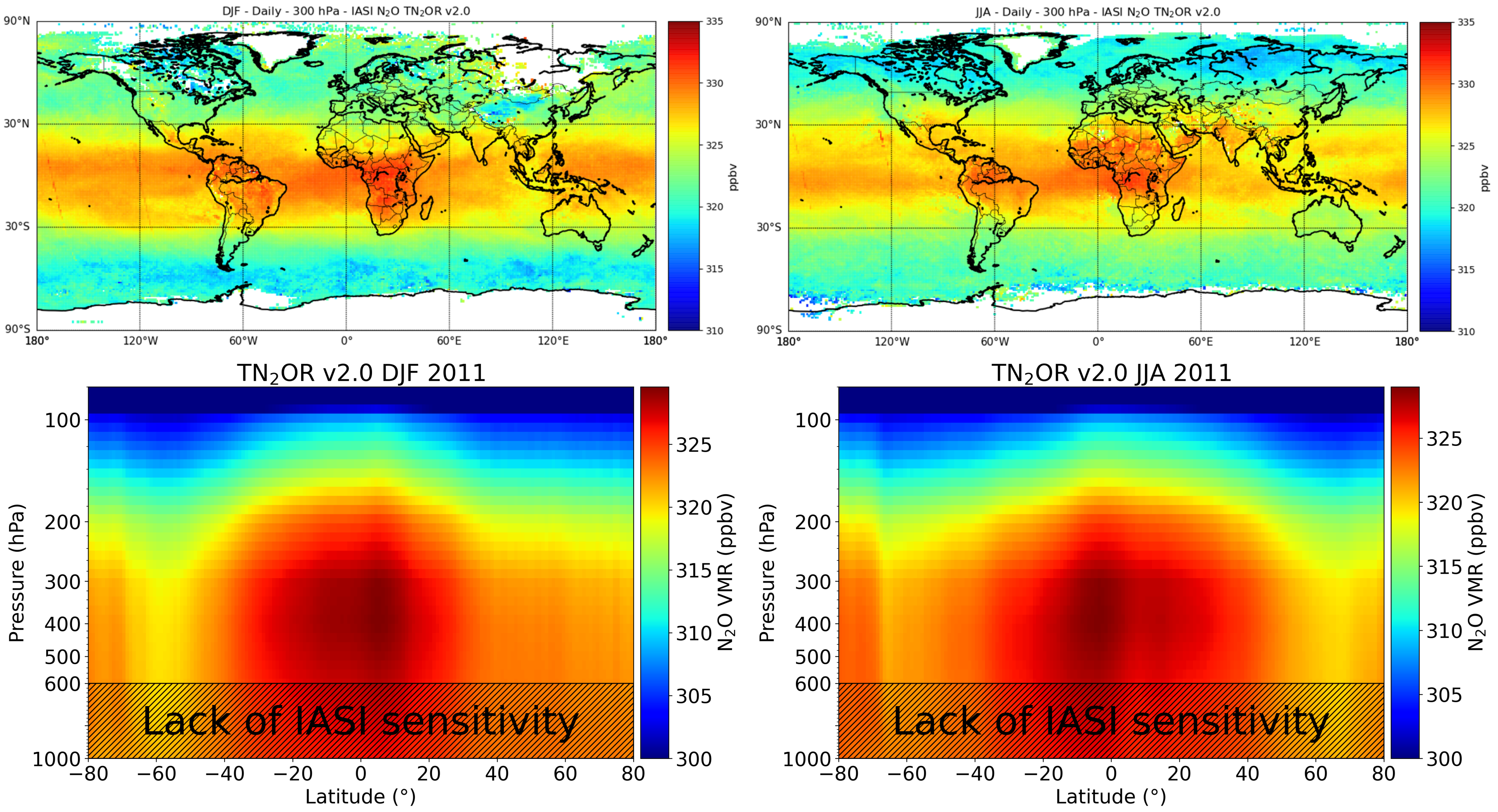
Differences between austral and boreal summers can be highlighted: (1) maxima of NO over South-Eastern USA in July 2011, and (2) maxima of NO over Australia in January 2011. The horizontal distributions of seasonally-averaged IASI NO estimated at 300 hPa in DJF and JJA 2011 at 1° × 1° horizontal resolution and the corresponding zonal cross sections are shown in Figure 14. We only consider these two seasons (winter and summer) to highlight the well marked differences in the NO distribution. Again, the general distribution of NO in the two seasons exhibits maxima in the tropics (around 330 ppbv) and minima in the high latitudes (315–318 ppbv). The maxima over equatorial Africa are systematically observed and then could be confirmed knowing that the tropical IASI NO is weakly low biased by (<−0.39 ppbv i.e., ∼0.1%) compared to aircraft observations (see Section 3). The African maximum was already studied in Ricaud et al. [10] and was attributed to the convergence of the Walker cells towards central Africa and to the strong upward transport associated with the deep convection bringing high surface NO emissions to the upper troposphere. Ricaud et al. [42] studied the distribution (July 2014) of chemical tracers such as carbon monoxide and aerosols between Africa and Southern America due to horizontal transport. Over the equatorial Atlantic Ocean in JJA, we show a tongue of NO maximum which can be likely explained by this horizontal transport. Local maxima of NO are also present over the Indian subcontinent and is slightly more intense in JJA when the Indian monsoon system pushes elevated amounts of NO from the surface to the upper troposphere to be trapped within the Asian Monsoon Anticyclone (see e.g., [8]). Over the tropics, we can note that there is systematically a minimum of NO over the Maritime Continent, the region encompassing Indonesia. Since this region represents one of the most efficient areas for transporting air masses from the surface to the upper troposphere (see e.g., [43,44]), the local minima observed at 300 hPa could be an imprint of NO-poor air masses in the lowermost troposphere over this area. In the middle latitudes, some local maxima over Mexico and the South East of the United States are depicted in JJA and, to a lesser extent, in SON (not shown). This is attributed to the presence of an anticyclone that traps NO-enriched air masses issued from the tropics (not shown). Finally the cross sections of zonal mean in Figure 14 clearly show the maximum of NO located more in the southern hemisphere in DJF and conversely more in the northern hemisphere in JJA following the location of the Intertropical Convergence Zone (ITCZ). Note also that the tropopause height is well marked with a maximum over the tropics and a minimum over high latitudes even if the IASI NO a priori is fixed with a tropopause height at 300 hPa (see Figure 3). This shows the impact of IASI measurements at this level. Conversely, there is a lack of sensitivity of IASI in the lowermost troposphere.
5. Conclusions
The Toulouse NO Retrieval Version 2.0 (TNOR v2.0) has been developed to especially retrieve NO profiles from the IASI spectral radiances. It is based on the RTTOV v12.3 model coupled to the Levenberg-Marquardt optimal estimation method. This enables also the simultaneous retrieval of CH, HO, temperature profiles together with surface temperature and emissivity within the 1240–1350 cm spectral window. The NO a priori vertical profile has been fixed over the time and location for the year 2011. This has the main advantage to state that any variation in the estimated IASI retrieval cannot be influenced by the impact of the a priori profile variation. The NO a priori profile is an average of several HIPPO profiles extrapolated by using LMDz-INCA model output. The NO a priori error was estimated at 0.8% from HIPPO aircraft data. The a priori vertical profiles of CH were taken from the MACC-II database at the closest location and time of the IASI observation. Our evaluation is focused on the upper-troposphere in which the retrieval level of 300 hPa has the most significant sensitivity. For one single retrieval, the total random error of IASI NO at 300 hPa has been found around 0.60% and also for 300–500 hPa in favorable conditions. The error decreases dramatically by averaging the data reaching 0.4 ppbv or 0.1% for a 1° × 1° box. The IASI NO data set has been evaluated against the aircraft NO observations from the HIPPO campaigns in 2009, 2010 and 2011 and the NOAA aircraft campaigns held in 2011, and also against the ground-based NO measurements from nine stations belonging to the NDACC network. We found values of global correlation coefficients of ∼0.77 between IASI and aircraft data. The bias between IASI and aircraft NO data is relatively small with ∼1.0 ppbv. We also found a similar bias at northern mid-latitudes of 0.97 ppbv and slightly higher at southern middle latitudes of 1.48 ppbv. At tropical latitudes, the bias is small but negative with values ranging between −0.4 and 0 ppbv. Finally, the estimated random error found with respect to the aircraft data is ∼2.3 ppbv (∼0.75%) similar to the total random error.
In the same way, the correlation between IASI and Northern Hemisphere NDACC stations (Kiruna, St Petersburg, Zugspitze, Jungfraujoch and Tenerife) is greater than 0.56 and could reach 0.85. The bias between IASI and NDACC data depends on the month but is generally small during summer for the northern hemisphere stations and quite constant over the year for the southern hemisphere stations (∼5 ppbv) except for Reunion island (∼7 ppbv). Moreover, the IASI variability is quite similar for Zugspitze and Jungfraujoch but usually twice less than the NDACC variability.
Finally, the distributions of IASI NO shown at 300 hPa at daily (0.2° × 0.2° horizontal resolution close to the IASI pixel size), monthly and seasonal time scale (1° × 1° horizontal resolution) exhibit maxima (>330 ppbv) over the tropics with hot spots over Central Africa and South America and minima (<318 ppbv) at high latitudes whatever the season and the time (day/night). A tongue of high NO over the equatorial Atlantic Ocean in JJA 2011 is likely attributed to horizontal transport between Africa and South America. Over the tropics, a minimum of NO is systematically observed over the Maritime Continent, the region encompassing Indonesia. In the middle latitudes, some local maxima over Mexico and the South East of the United States are depicted in JJA 2011 likely attributed to the presence of an anticyclone that traps NO-enriched air masses issued from the tropics. Differences between austral and boreal summers can also be highlighted by: (1) maxima of NO over South-Eastern USA in July 2011, and (2) maxima of NO over Australia in January 2011. In addition, the vertical structure of IASI NO shows a clear delimitation between the troposphere and the stratosphere despite a fixed a priori profile. Considering the rather weak random and systematic errors evaluated over the different continents, this new set of IASI NO data, with its realistic distribution, could be used for future on going research to retrieve the emission sources by model inversion.
Supplementary Materials
The following supporting information can be downloaded at https://www.mdpi.com/article/10.3390/rs14061403/s1. Figure S1: A priori () (blue) and retrieved () (red) radiance residuals for the 24 pixels observed in and presented in Table 1 and Figure 1. Figure S2: NO averaging kernels calculated with TNOR v2.0 over the 13-level retrieval grid selected for the 24 pixels measured and presented in Table 1 and Figure 1. Figure S3: Radiance perturbated by 1% of NO, CH, HO profiles and surface emissivity, and 1 K of temperature profile and surface temperature variation, parameters retrieved with TNOR v2.0, for the 24 pixels measured and presented in Table 1 and Figure 1. Figure S4: Vertical distribution of the measurement error (%, red), smoothing error (%, blue) and total error (%, black) of the NO retrieved with TNOR v2.0 for the 24 pixels selected and presented in Table 1 and Figure 1. Figure S5; Vertical distribution of the contamination factors induced of the parameters, other than NO, retrieved with TNOR v2.0 and affecting the NO retrieval for the 24 pixels selected and presented in Table 1 and Figure 1: Temperature (red), HO (blue), CH (green), surface temperature (orange) and surface emissivity (purple). Figure S6: Representative NO IASI (blue) and NDACC (red) a priori vertical profiles concerning the 9 NDACC stations presented in Table 4 and Figure 1 for specific months for each NDACC stations. Figure S7: Representative monthly-averaged NO averaging kernels of IASI computed with TNOR v2.0 (above) and NDACC FTIR instruments (below) above the 9 selected NDACC stations presented in Table 4 and Figure 1 for specific months for each NDACC stations.
Author Contributions
Conceptualization, R.C., J.-L.A. and P.R.; data curaction, R.C.; formal analysis, R.C.; funding acquisition, J.-L.A. and P.R.; investigation, R.C.; methodology, R.C.; project administration, J.-L.A. and P.R.; resources, J.V. and D.H.; software, R.C., J.V. and Y.K.; supervision, J.-L.A. and P.R.; validation, R.C., J.-L.A. and P.R.; visualization, R.T.; writing—original draft, R.C., J.-L.A. and P.R.; writing—review and editing, R.C., J.-L.A., P.R., Y.K. and J.V. All authors have read and agreed to the published version of the manuscript.
Funding
The TNOR project is funded by the Région Occitanie, the University of Toulouse, the Institut National des Sciences de l’Univers (INSU)/Centre National de la Recherche Scientifique (CNRS), Météo-France, the Centre National d’Etudes Spatiales (CNES), Airbus Defense and Space, and Sciences et technologies pour l’Aéronautique et l’Espace (STAE) foundation. RC’s PhD has been funded by Région Occitanie, Airbus Defense and Space, and STAE.
Data Availability Statement
The TNOR IASI NO data are available on request to J.-L. Attié and P. Ricaud.
Acknowledgments
We would like to thank C. Sweeney (National Oceanic and Atmospheric Administration (NOAA), Global Monitoring Laboratory, Earth System Research Laboratories; Boulder, CO 80305, USA) for providing us with NOAA Global Greenhouse Gas Reference Network (GGGRN) Aircraft data in 2011 as well as his valuable comments on the paper, the National Center for Atmospheric Research (NCAR) for the HIPPO data as open source (https://www.eol.ucar.edu/, accessed on 18 February 2022), EUMETSAT for the IASI level 1C and level 2 data as open source (https://www.eumetsat.int/iasi/, accessed on 18 February 2022), ECMWF for the CH MACC data as open source (https://apps.ecmwf.int/, accessed on 31 August 2021) and the NDACC for the NO FTIR data as open source (http://ndaccdemo.org/, accessed on 18 February 2022). We also thank the three anonymous reviewers for their encouraging and valuable comments that contribute to improve the paper.
Conflicts of Interest
The authors declare no conflict of interest.
References
- Prather, M.J.; Hsu, J.; DeLuca, N.M.; Jackman, C.H.; Oman, L.D.; Douglass, A.R.; Fleming, E.L.; Strahan, S.E.; Steenrod, S.D.; Søvde, O.A.; et al. Measuring and modeling the lifetime of nitrous oxide including its variability. J. Geophys. Res. Atmos. 2015, 120, 5693–5705. [Google Scholar] [CrossRef] [PubMed]
- Stocker, T. Climate Change 2013: The Physical Science Basis: Working Group I Contribution to the Fifth Assessment Report of the Intergovernmental Panel on Climate Change; Cambridge University Press: Cambridge, UK, 2014. [Google Scholar]
- Ravishankara, A.; Daniel, J.S.; Portmann, R.W. Nitrous oxide (N2O): The dominant ozone-depleting substance emitted in the 21st century. Science 2009, 326, 123–125. [Google Scholar] [CrossRef] [PubMed] [Green Version]
- Tian, H.; Xu, R.; Canadell, J.G.; Thompson, R.L.; Winiwarter, W.; Suntharalingam, P.; Davidson, E.A.; Ciais, P.; Jackson, R.B.; Janssens-Maenhout, G.; et al. A comprehensive quantification of global nitrous oxide sources and sinks. Nature 2020, 586, 248–256. [Google Scholar] [CrossRef] [PubMed]
- Bakker, D.C.; Bange, H.W.; Gruber, N.; Johannessen, T.; Upstill-Goddard, R.C.; Borges, A.V.; Delille, B.; Löscher, C.R.; Naqvi, S.; Omar, A.M.; et al. Air-sea interactions of natural long-lived greenhouse gases (CO2, N2O, CH4) in a changing climate. In Ocean-Atmosphere Interactions of Gases and Particles; Springer: Berlin/Heidelberg, Germany, 2014. [Google Scholar]
- Minschwaner, K.; Salawitch, R.; McElroy, M. Absorption of solar radiation by O2: Implications for O3 and lifetimes of N2O, CFCl3, and CF2Cl2. J. Geophys. Res. Atmos. 1993, 98, 10543–10561. [Google Scholar] [CrossRef]
- Xiong, X.; Maddy, E.S.; Barnet, C.; Gambacorta, A.; Patra, P.K.; Sun, F.; Goldberg, M. Retrieval of nitrous oxide from Atmospheric Infrared Sounder: Characterization and validation. J. Geophys. Res. Atmos. 2014, 119, 9107–9122. [Google Scholar] [CrossRef]
- Kangah, Y.; Ricaud, P.; Attié, J.L.; Saitoh, N.; Hauglustaine, D.A.; Wang, R.; El Amraoui, L.; Zbinden, R.; Delon, C. Summertime upper tropospheric nitrous oxide over the Mediterranean as a footprint of Asian emissions. J. Geophys. Res. Atmos. 2017, 122, 4746–4759. [Google Scholar] [CrossRef]
- García, O.E.; Schneider, M.; Ertl, B.; Sepúlveda, E.; Borger, C.; Diekmann, C.; Wiegele, A.; Hase, F.; Barthlott, S.; Blumenstock, T.; et al. The MUSICA IASI CH4 and N2O products and their comparison to HIPPO, GAW and NDACC FTIR references. Atmos. Meas. Tech. 2018, 11, 4171–4215. [Google Scholar] [CrossRef] [Green Version]
- Ricaud, P.; Attié, J.L.; Teyssèdre, H.; Amraoui, L.E.; Peuch, V.H.; Matricardi, M.; Schluessel, P. Equatorial total column of nitrous oxide as measured by IASI on MetOp-A: Implications for transport processes. Atmos. Chem. Phys. 2009, 9, 3947–3956. [Google Scholar] [CrossRef] [Green Version]
- Ricaud, P.; Sič, B.; El Amraoui, L.; Attié, J.L.; Zbinden, R.; Huszar, P.; Szopa, S.; Parmentier, J.; Jaidan, N.; Michou, M.; et al. Impact of the Asian monsoon anticyclone on the variability of mid-to-upper tropospheric methane above the Mediterranean Basin. Atmos. Chem. Phys. 2014, 14, 11427–11446. [Google Scholar] [CrossRef] [Green Version]
- García, O.E.; Sepúlveda, E.; Schneider, M.; Hase, F.; August, T.; Blumenstock, T.; Kühl, S.; Munro, R.; Gómez-Peláez, Á.J.; Hultberg, T.; et al. Consistency and quality assessment of the Metop-A/IASI and Metop-B/IASI operational trace gas products (O3, CO, N2O, CH4, and CO2) in the subtropical North Atlantic. Atmos. Meas. Tech. 2016, 9, 2315–2333. [Google Scholar] [CrossRef] [Green Version]
- Turquety, S.; Hadji-Lazaro, J.; Clerbaux, C.; Hauglustaine, D.; Clough, S.; Cassé, V.; Schlüssel, P.; Mégie, G. Operational trace gas retrieval algorithm for the Infrared Atmospheric Sounding Interferometer. J. Geophys. Res. Atmos. 2004, 109. [Google Scholar] [CrossRef]
- Kangah, K.G.Y. Mesure du Protoxyde D’azote (N2O) Depuis l’espace. Ph.D. Thesis, Université Paul Sabatier-Toulouse III, Toulouse, France, 2017. [Google Scholar]
- Barret, B.; Gouzenes, Y.; Le Flochmoen, E.; Ferrant, S. Retrieval of Metop-A/IASI N2O profiles and validation with NDACC FTIR data. Atmosphere 2021, 12, 219. [Google Scholar] [CrossRef]
- Hilton, F.; Armante, R.; August, T.; Barnet, C.; Bouchard, A.; Camy-Peyret, C.; Capelle, V.; Clarisse, L.; Clerbaux, C.; Coheur, P.F.; et al. Hyperspectral Earth observation from IASI: Five years of accomplishments. Bull. Am. Meteorol. Soc. 2012, 93, 347–370. [Google Scholar] [CrossRef]
- Pougatchev, N.; August, T.; Calbet, X.; Hultberg, T.; Oduleye, O.; Schlüssel, P.; Stiller, B.; Germain, K.S.; Bingham, G. IASI temperature and water vapor retrievals—Error assessment and validation. Atmos. Chem. Phys. 2009, 9, 6453–6458. [Google Scholar] [CrossRef] [Green Version]
- Rodgers, C.D. Inverse Methods for Atmospheric Sounding: Theory and Practice; World Scientific: Singapore, 2000; Volume 2. [Google Scholar]
- Dufour, G.; Eremenko, M.; Griesfeller, A.; Barret, B.; LeFlochmoën, E.; Clerbaux, C.; Hadji-Lazaro, J.; Coheur, P.F.; Hurtmans, D. Validation of three different scientific ozone products retrieved from IASI spectra using ozonesondes. Atmos. Meas. Tech. 2012, 5, 611–630. [Google Scholar] [CrossRef] [Green Version]
- Wofsy, S.C. HIAPER Pole-to-Pole Observations (HIPPO): Fine-grained, global-scale measurements of climatically important atmospheric gases and aerosols. Philos. Trans. R. Soc. A 2011, 369, 2073–2086. [Google Scholar] [CrossRef]
- Wofsy, S.C.; Daube, B.C.; Jimenez, R.; Kort, E.; Pittman, J.V.; Park, S.; Commane, R.; Xiang, B.; Santoni, G.; Jacob, D.; et al. HIPPO Merged 10-Second Meteorology and Atmospheric Chemistry and Aerosol Data (R_20121129). Philos. Trans. R. Soc. A 2012. [Google Scholar] [CrossRef]
- Hauglustaine, D.; Hourdin, F.; Jourdain, L.; Filiberti, M.A.; Walters, S.; Lamarque, J.F.; Holland, E. Interactive chemistry in the Laboratoire de Météorologie Dynamique general circulation model: Description and background tropospheric chemistry evaluation. J. Geophys. Res. Atmos. 2004, 109. [Google Scholar] [CrossRef]
- Kort, E.; Patra, P.; Ishijima, K.; Daube, B.; Jimenez, R.; Elkins, J.; Hurst, D.; Moore, F.; Sweeney, C.; Wofsy, S. Tropospheric distribution and variability of N2O: Evidence for strong tropical emissions. Geophys. Res. Lett. 2011, 38. [Google Scholar] [CrossRef] [Green Version]
- Sweeney, C.; Karion, A.; Wolter, S.; Newberger, T.; Guenther, D.; Higgs, J.A.; Andrews, A.E.; Lang, P.M.; Neff, D.; Dlugokencky, E.; et al. Seasonal climatology of CO2 across North America from aircraft measurements in the NOAA/ESRL Global Greenhouse Gas Reference Network. J. Geophys. Res. Atmos. 2015, 120, 5155–5190. [Google Scholar] [CrossRef]
- Sepúlveda, E.; Schneider, M.; Hase, F.; Barthlott, S.; Dubravica, D.; García, O.E.; Gomez-Pelaez, A.; González, Y.; Guerra, J.C.; Gisi, M.; et al. Tropospheric CH4 signals as observed by NDACC FTIR at globally distributed sites and comparison to GAW surface in situ measurements. Atmos. Meas. Tech. 2014, 7, 2337–2360. [Google Scholar] [CrossRef] [Green Version]
- Saunders, R.; Matricardi, M.; Brunel, P. An improved fast radiative transfer model for assimilation of satellite radiance observations. Q. J. R. Meteorol. Soc. 1999, 125, 1407–1425. [Google Scholar] [CrossRef]
- Saunders, R.; Hocking, J.; Turner, E.; Rayer, P.; Rundle, D.; Brunel, P.; Vidot, J.; Roquet, P.; Matricardi, M.; Geer, A.; et al. An update on the RTTOV fast radiative transfer model (currently at version 12). Geosci. Model Dev. 2018, 11, 2717–2737. [Google Scholar] [CrossRef] [Green Version]
- Hocking, J.; Rayer, P.; Rundle, D.; Saunders, R.; Matricardi, M.; Geer, A.; Brunel, P.; Vidot, J. RTTOV v11 Users Guide; Met-Office, ECMWF, Météo-France: Paris, France, 2015. [Google Scholar]
- Matricardi, M. An assessment of the accuracy of the RTTOV fast radiative transfer model using IASI data. Atmos. Chem. Phys. 2009, 9, 6899–6913. [Google Scholar] [CrossRef] [Green Version]
- Matricardi, M. The Generation of RTTOV Regression Coefficients for IASI and AIRS Using a New Profile Training Set and a New Line-by-Line Database; ECMWF Reading: Reading, UK, 2008. [Google Scholar]
- Saunders, R.; Hocking, J.; Rundle, D.; Rayer, P.; Havemann, S.; Matricardi, M.; Geer, A.; Lupu, C.; Brunel, P.; Vidot, J. RTTOV-12: Science and Validation Report; Met-Office, ECMWF, Météo-France: Paris, France, 2017. [Google Scholar]
- Chevallier, F.; Di Michele, S.; McNally, A.P. Diverse Profile Datasets from the ECMWF 91-Level Short-Range Forecasts; European Centre for Medium-Range Weather Forecasts: Reading, UK, 2006. [Google Scholar]
- Ricaud, P.; Attié, J.L.; Chalinel, R.; Pasternak, F.; Léonard, J.; Pison, I.; Pattey, E.; Thompson, R.L.; Zelinger, Z.; Lelieveld, J.; et al. The Monitoring Nitrous Oxide Sources (MIN2OS) satellite project. Remote Sens. Environ. 2021, 266, 112688. [Google Scholar] [CrossRef]
- Levenberg, K. A method for the solution of certain non-linear problems in least squares. Q. Appl. Math. 1944, 2, 164–168. [Google Scholar] [CrossRef] [Green Version]
- Marquardt, D.W. An algorithm for least-squares estimation of nonlinear parameters. J. Soc. Ind. Appl. Math. 1963, 11, 431–441. [Google Scholar] [CrossRef]
- Massart, S.; Agusti-Panareda, A.; Aben, I.; Butz, A.; Chevallier, F.; Crevoisier, C.; Engelen, R.; Frankenberg, C.; Hasekamp, O. Assimilation of atmospheric methane products into the MACC-II system: from SCIAMACHY to TANSO and IASI. Atmos. Chem. Phys. 2014, 14, 6139–6158. [Google Scholar] [CrossRef] [Green Version]
- Loveless, M.; Borbas, E.E.; Knuteson, R.; Cawse-Nicholson, K.; Hulley, G.; Hook, S. Climatology of the Combined ASTER MODIS Emissivity over Land (CAMEL) Version 2. Remote Sens. 2021, 13, 111. [Google Scholar] [CrossRef]
- Konda, M.; Imasato, N.; Nishi, K.; Toda, T. Measurement of the sea surface emissivity. J. Oceanogr. 1994, 50, 17–30. [Google Scholar] [CrossRef]
- Clarisse, L.; Coheur, P.F.; Prata, F.; Hadji-Lazaro, J.; Hurtmans, D.; Clerbaux, C. A unified approach to infrared aerosol remote sensing and type specification. Atmos. Chem. Phys. 2013, 13, 2195–2221. [Google Scholar] [CrossRef] [Green Version]
- Cuesta, J.; Eremenko, M.; Flamant, C.; Dufour, G.; Laurent, B.; Bergametti, G.; Höpfner, M.; Orphal, J.; Zhou, D. Three-dimensional distribution of a major desert dust outbreak over East Asia in March 2008 derived from IASI satellite observations. J. Geophys. Res. Atmos. 2015, 120, 7099–7127. [Google Scholar] [CrossRef] [Green Version]
- Rodgers, C.D.; Connor, B.J. Intercomparison of remote sounding instruments. J. Geophys. Res. Atmos. 2003, 108. [Google Scholar] [CrossRef] [Green Version]
- Ricaud, P.; Zbinden, R.; Catoire, V.; Brocchi, V.; Dulac, F.; Hamonou, E.; Canonici, J.C.; El Amraoui, L.; Massart, S.; Piguet, B.; et al. The GLAM Airborne Campaign across the Mediterranean Basin. Bull. Am. Meteorol. Soc. 2018, 99, 361–380. [Google Scholar] [CrossRef] [Green Version]
- Liu, C.; Zipser, E.J. Global distribution of convection penetrating the tropical tropopause. J. Geophys. Res. Atmos. 2005, 110. [Google Scholar] [CrossRef] [Green Version]
- Dion, I.A.; Ricaud, P.; Haynes, P.; Carminati, F.; Dauhut, T. Ice injected into the tropopause by deep convection—Part 1: In the austral convective tropics. Atmos. Chem. Phys. 2019, 19, 6459–6479. [Google Scholar] [CrossRef] [Green Version]
Figure 1.
Locations of the observations used to assess the quality of the IASI NO data: NDACC ground-based stations (orange stars), HIPPO airborne measurements in 2009 (red circles), 2010 (green circles) and 2011 (blue circles), and the NOAA airborne campaigns in 2011 (black and white stars). Also shown is the location of the 24 IASI pixels (red triangles for June, July or August and blue triangles for December, January or February 2011. Dates and times of observations are listed in Table 1.
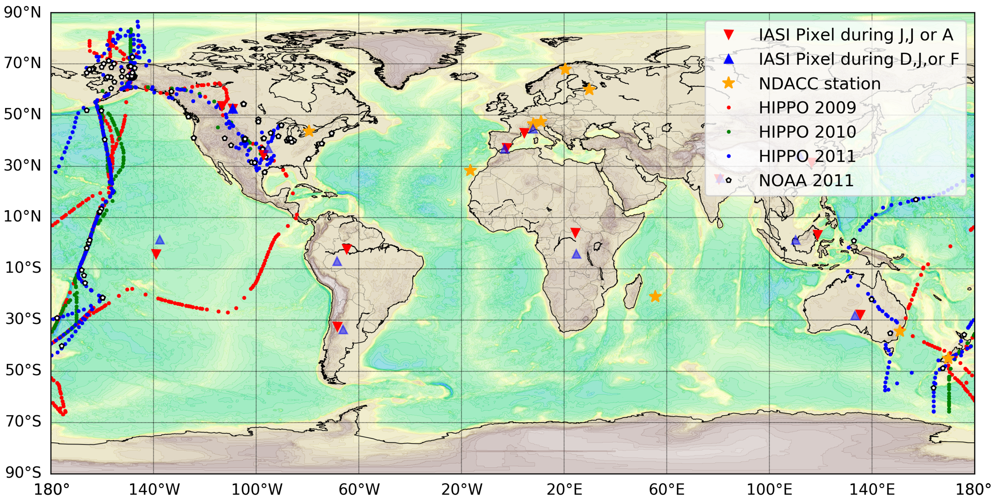
Figure 2.
Brightness temperature sensitivity defined as the absolute change in brightness temperature (BT|) for 1% change (left panel): HO (dark blue), CH (green), and NO (black) and (right panel): surface emissivity (purple) and for 1 K change in: temperature profile (red), surface temperature (orange) for one pixel selected over France in summer daytime. No data represent channels not selected. Note that the y axis is in logarithmic scale.
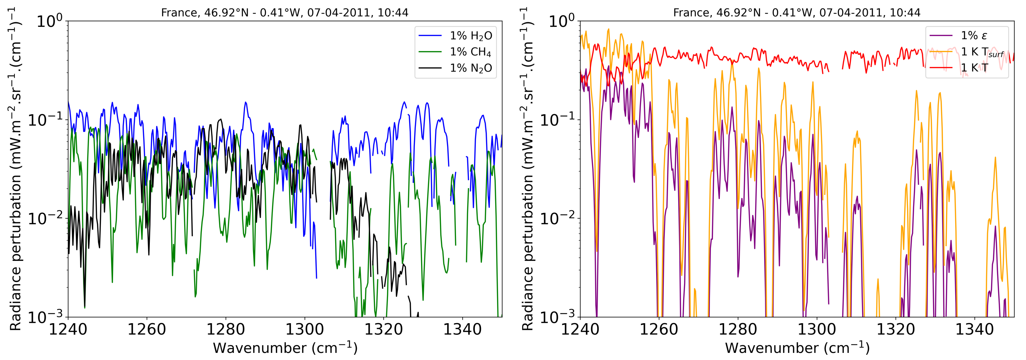
Figure 3.
(Left) N (N = 854) HIPPO NO vertical profiles measured during the 5 campaigns (2009–2011), together with its mean (black) and standard deviation (±1, red). (Right) A priori NO vertical profile used in TNOR v2.0 and its associated error (±0.8%, horizontal arrow) taken from the HIPPO mean and its associated standard deviation.
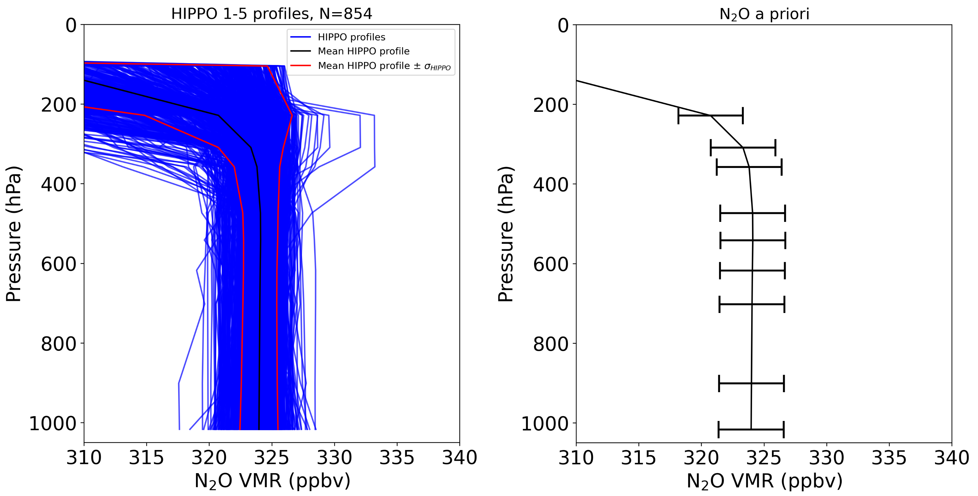
Figure 4.
A priori (blue) and retrieved (red) radiance residuals for 3 pixels observed over France (8 February 2011), Pacific Ocean (12 June 2011) and over USA (15 February 2011). The IASI spectral noise is represented by the 2 solid black lines. Missing data represent channels not selected.
Figure 4.
A priori (blue) and retrieved (red) radiance residuals for 3 pixels observed over France (8 February 2011), Pacific Ocean (12 June 2011) and over USA (15 February 2011). The IASI spectral noise is represented by the 2 solid black lines. Missing data represent channels not selected.

Figure 5.
Horizontal distribution of the Degrees of Freedom of Signal (DOFS) on a 1° × 1° grid obtained with TNOR v2.0 for: daytime and nighttime NO in left column and right column, respectively. DJF 2011 and (top) JJA 2011 (bottom). The pixels were selected with DOFS values greater than 0.9.
Figure 5.
Horizontal distribution of the Degrees of Freedom of Signal (DOFS) on a 1° × 1° grid obtained with TNOR v2.0 for: daytime and nighttime NO in left column and right column, respectively. DJF 2011 and (top) JJA 2011 (bottom). The pixels were selected with DOFS values greater than 0.9.
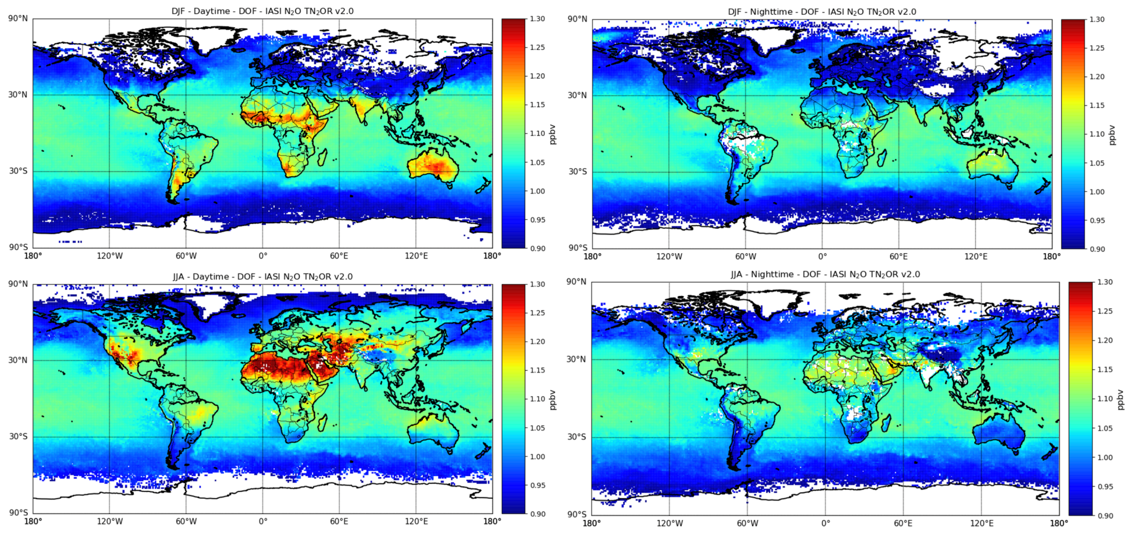
Figure 6.
Example of NO averaging kernels (left), errors in % (middle) and contamination factors in % (right) calculated with TNOR v2.0 on 13 retrieval levels over France during summer daytime (27 August 2011). The levels of the averaging kernels are defined by the different colors presented within the left panel. The retrieval noise (%, red) and smoothing errors (%, blue) are presented on the middle figure as well as the total random error (%, black) on one single retrieval. The contamination factors (%) affecting the NO retrievals induced by: HO (dark blue), CH (green), temperature (red), surface temperature (orange) and emissivity (purple) are shown.

Figure 7.
IASI NO distribution (left) and IASI NO total error (right) in ppbv at 300 hPa for 1 August 2011 within a box of 1° × 1°.
Figure 7.
IASI NO distribution (left) and IASI NO total error (right) in ppbv at 300 hPa for 1 August 2011 within a box of 1° × 1°.

Figure 8.
(Left): Scatter plot between aircraft NO observations from HIPPO and NOAA campaigns convolved with the appropriate averaging kernels vs IASI NO retrievals at 300 hPa covering the period from 2009 to 2011. The red and blue circles stands for the aircraft and IASI data, respectively. The correlation R, bias and standard deviations of IASI and aircraft observations are presented together with the standard deviation of the difference between IASI and aircraft for collocated profiles. (Right): Comparison between aircraft and IASI NO along the latitude for 300 hPa. The red × sign stands for the aircraft data and the blue + sign stands for IASI data averages over 30° latitudes. The red and blue curves represent a sinusoidal fit applied to aircraft and IASI data, respectively. The grey areas represent 95% C.I.

Figure 9.
Monthly NO evolution of IASI and aircraft data in ppbv for 2011 at 300 hPa. The red × sign stands for the aircraft data and the blue + sign stands for IASI data. The vertical bars represent the standard deviation for each monthly NO average. The purple bins represent the positive monthly bias and the golden bins represent the negative monthly bias. Note that the right axis shows the absolute value of the bias. The thin black line represents the value of the IASI NO fixed a priori.
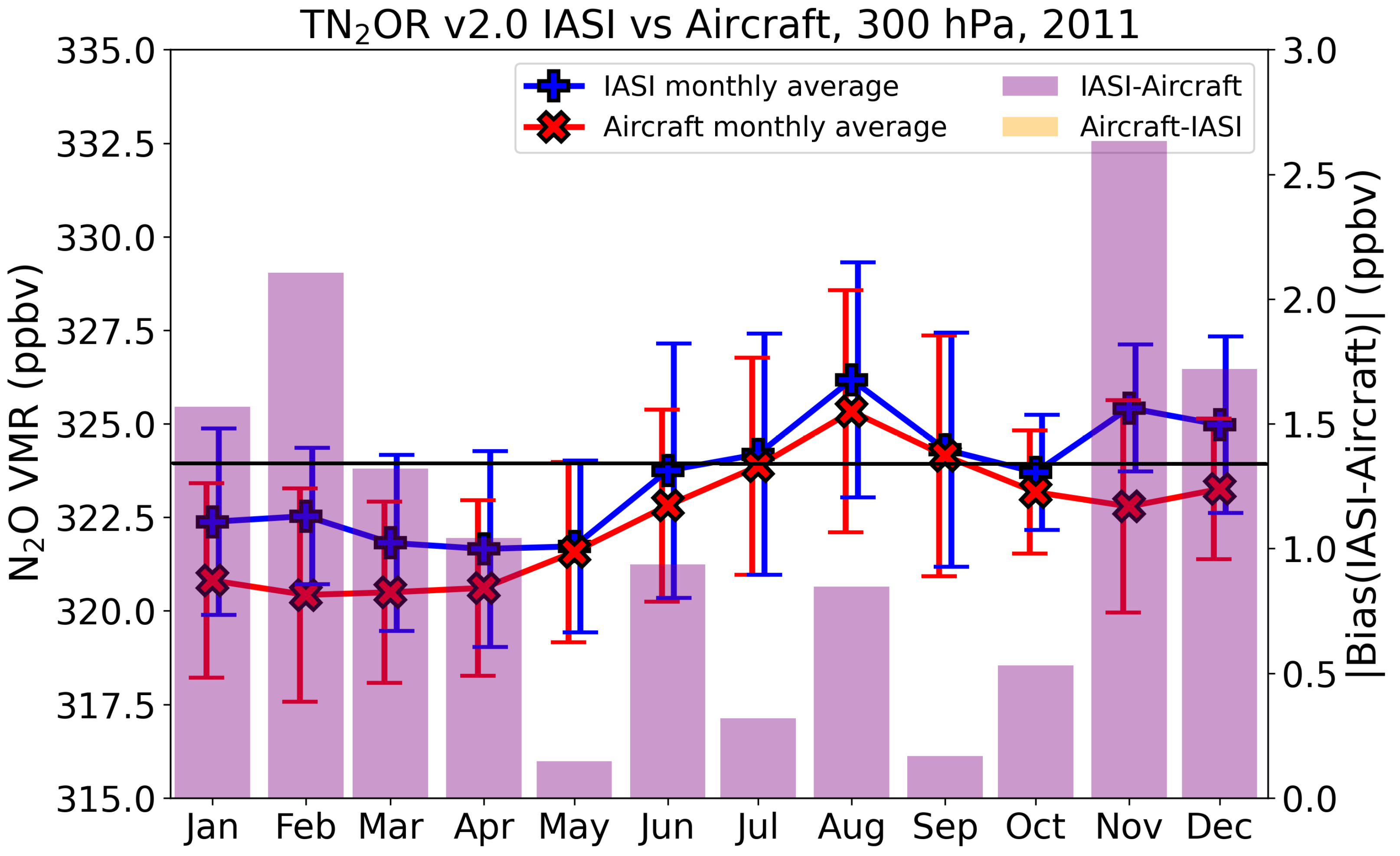
Figure 10.
(Top): Monthly-averaged NO averaging kernels in July 2011 above St Petersburg, Russia and Wollongong, Australia stations from the NDACC FTIR instruments. (Bottom): Same as top panels but for the corresponding IASI data.
Figure 10.
(Top): Monthly-averaged NO averaging kernels in July 2011 above St Petersburg, Russia and Wollongong, Australia stations from the NDACC FTIR instruments. (Bottom): Same as top panels but for the corresponding IASI data.

Figure 11.
Monthly evolution of NO above the selected NDACC FTIR stations over January–December 2011 at 300 hPa. Note that Equation (9) has been applied to NDACC NO data. The a priori used in the NDACC (dotted red) and IASI (dotted blue) retrievals are also shown. Vertical thick lines represent standard deviation on the monthly mean. The purple bins represent the positive monthly bias and the golden bins represent the negative monthly bias. Note that the right axis shows the absolute value of the bias which is between 0 to 20 ppbv.
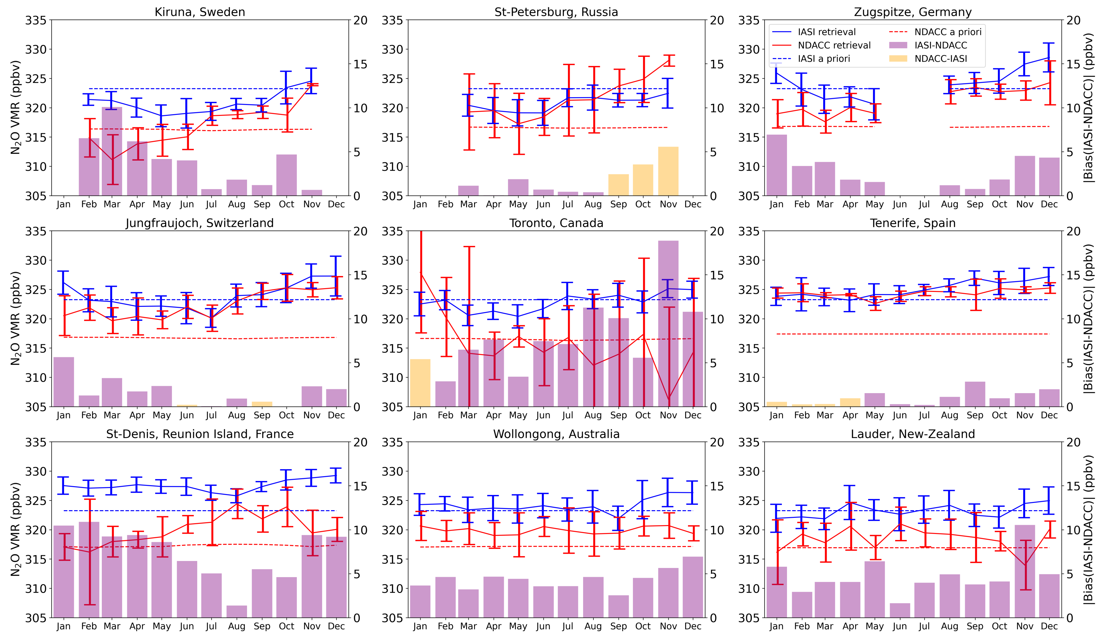
Figure 12.
Horizontal distribution of daily-averaged NO at 300 hPa from IASI on 1 August 2011 within 0.2° × 0.2° pixels.
Figure 12.
Horizontal distribution of daily-averaged NO at 300 hPa from IASI on 1 August 2011 within 0.2° × 0.2° pixels.
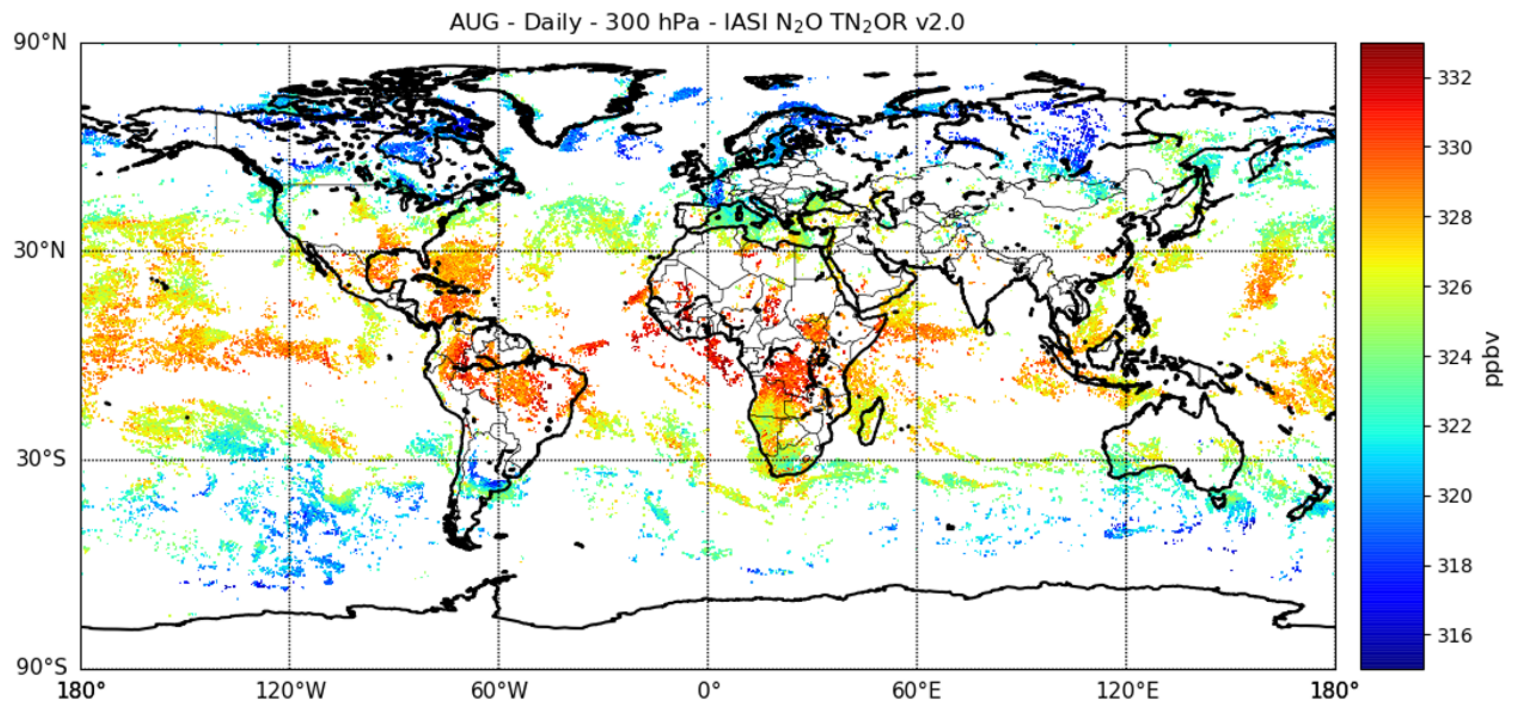
Figure 13.
Horizontal distribution of monthly-averaged NO (both daytime and nighttime) at 300 hPa from IASI in January 2011 (left) and in July 2011 (right) within a 1° × 1° box.
Figure 13.
Horizontal distribution of monthly-averaged NO (both daytime and nighttime) at 300 hPa from IASI in January 2011 (left) and in July 2011 (right) within a 1° × 1° box.

Figure 14.
Horizontal distribution of IASI NO from TNOR v2.0 at 300 hPa within 1° × 1° box and zonal mean vertical cross-section of NO for DJF (top left and bottom left) and JJA (top right and bottom right). The hatched area is an indication where the sensitivity profile of IASI is weak.
Figure 14.
Horizontal distribution of IASI NO from TNOR v2.0 at 300 hPa within 1° × 1° box and zonal mean vertical cross-section of NO for DJF (top left and bottom left) and JJA (top right and bottom right). The hatched area is an indication where the sensitivity profile of IASI is weak.

Table 1.
Location, latitude, longitude, date, time, and surface pressure of the 24 IASI pixels used in our study measured in different periods. The 24 IASI pixels are also shown in Figure 1.
Table 1.
Location, latitude, longitude, date, time, and surface pressure of the 24 IASI pixels used in our study measured in different periods. The 24 IASI pixels are also shown in Figure 1.
| Pixel # | Location | Latitude | Longitude | Date /2011 | Time /UT | Surface P. /hPa |
|---|---|---|---|---|---|---|
| 1 | Canada | 52.55°N | 109.13°W | 11 June | 17:04 | 934.7 |
| 2 | 53.48°N | 113.35°W | 24 December | 04:50 | 936.54 | |
| 3 | France | 46.92°N | 0.41°W | 4 July | 10:44 | 998.73 |
| 4 | 49.51°N | 1.89°E | 8 February | 11:04 | 1008.69 | |
| 5 | Spain | 36.94°N | 3.11°W | 25 August | 09:30 | 979.8 |
| 6 | 37.14°N | 2.41°W | 23 February | 09:17 | 939.8 | |
| 7 | USA | 37.09°N | 95.41°W | 15 June | 15:44 | 977.8 |
| 8 | 34.41°N | 97.23°W | 15 February | 17:08 | 984.37 | |
| 9 | China | 34.55°N | 111.68°E | 7 June | 01:39 | 944.15 |
| 10 | 31.46°N | 116.41°E | 2 December | 02:49 | 1005.02 | |
| 11 | India | 25.45°N | 80.92°E | 7 June | 05:04 | 977.2 |
| 12 | 24.99°N | 80.37°E | 26 February | 04:54 | 977.35 | |
| 13 | Congo Rainforest | 4.09°S | 24.77°E | 7 July | 08:14 | 943.86 |
| 14 | 4.11°N | 24.43°E | 16 February | 08:29 | 944.33 | |
| 15 | Indonesia | 1.28°N | 110.2°E | 24 August | 01:35 | 985.84 |
| 16 | 3.22°N | 118.82°E | 8 January | 12:53 | 1007.02 | |
| 17 | Pacific ocean | 1.45°N | 137.59°W | 12 June | 06:00 | 1010.93 |
| 18 | 4.28°S | 139.03°W | 5 December | 06:09 | 1012.0 | |
| 19 | Amazonia | 6.96°S | 68.43°W | 11 August | 14:36 | 1000.62 |
| 20 | 2.32°S | 64.77°W | 30 December | 13:29 | 1003.5 | |
| 21 | Australia | 28.2°S | 133.35°E | 31 August | 00:57 | 990.16 |
| 22 | 27.9°S | 135.42°E | 2 December | 23:24 | 992.41 | |
| 23 | Argentina | 33.62°S | 66.15°W | 22 August | 14:15 | 960.27 |
| 24 | 32.57°S | 68.4°W | 24 December | 14:01 | 948.56 |
Table 2.
A priori information and error for NO, CH, HO, and temperature (Temp) profiles, surface temperature (T) and emissivity (). The emissivity a priori is issued from the MEaSUREs CAMEL atlas for land surface [31] and from Konda et al. [38] for sea surface.
| Parameters | NO | CH | HO | Temp | T | |
|---|---|---|---|---|---|---|
| A priori | From HIPPO and LMDz-INCA | MACC-II | IASI | IASI | IASI | CAMEL (land) 0.984 (sea) |
| x | 0.8% | 1% | 10% | 0.5 K | 1.5 K | 15% |
Table 3.
Standard deviation of NO () in IASI and aircraft data sets, correlation R and bias (ppbv) between the IASI and aircraft data sets at 300 hPa as a function of latitude bands, together with the number of profiles (N) used in the statistics. Note that aircraft data have been convolved with the appropriate IASI averaging kernels.
| Latitudes | N | (ppbv) | (ppbv) | R | Bias (ppbv) |
|---|---|---|---|---|---|
| 60°S–30°S | 45 | 2.36 | 2.69 | 0.76 | 1.48 |
| 30°S–0° | 60 | 1.82 | 1.92 | 0.61 | −0.03 |
| 0°–30°N | 64 | 2.13 | 1.42 | 0.56 | −0.39 |
| 30°N–60°N | 328 | 2.91 | 2.63 | 0.71 | 0.97 |
| 60°N–90°N | 95 | 1.93 | 2.19 | 0.13 | 2.56 |
Table 4.
Location of the NDACC stations used to evaluate the quality of the IASI NO retrievals. Correlation coefficient R, bias (IASI NO-NDACC NO) between IASI and NDACC and their corresponding standard deviation for 300 hPa.
Table 4.
Location of the NDACC stations used to evaluate the quality of the IASI NO retrievals. Correlation coefficient R, bias (IASI NO-NDACC NO) between IASI and NDACC and their corresponding standard deviation for 300 hPa.
| Station | Lat | Lon | H (m amsl) | R | Bias (ppbv) | (ppbv) | |
|---|---|---|---|---|---|---|---|
| IASI | NDACC | ||||||
| Kiruna | 67.84°N | 20.41°E | 419 | 0.56 | 4.0 | 1.8 | 3.48 |
| St Petersburg | 59.9°N | 29.8°E | 20 | 0.85 | −0.78 | 1.17 | 3.25 |
| Zugspitze | 47.42°N | 10.98°E | 2964 | 0.69 | 3.01 | 2.45 | 2.19 |
| Jungfraujoch | 46.55°N | 7.98°E | 3580 | 0.7 | 1.56 | 2.16 | 2.16 |
| Toronto | 43.66°N | 79.40°W | 174 | −0.28 | 7.18 | 1.51 | 4.93 |
| Tenerife | 28.30°N | 16.48°W | 2367 | 0.56 | 0.7 | 1.32 | 0.68 |
| St-Denis | 20.9°S | 55.5°E | 85 | −0.16 | 7.51 | 0.94 | 2.45 |
| Wollongong | 34.41°S | 150.88°E | 30 | 0.38 | 4.33 | 1.2 | 0.61 |
| Lauder | 45.04°S | 169.68°E | 370 | 0.1 | 4.76 | 1.09 | 1.92 |
Publisher’s Note: MDPI stays neutral with regard to jurisdictional claims in published maps and institutional affiliations. |
© 2022 by the authors. Licensee MDPI, Basel, Switzerland. This article is an open access article distributed under the terms and conditions of the Creative Commons Attribution (CC BY) license (https://creativecommons.org/licenses/by/4.0/).
Share and Cite
MDPI and ACS Style
Chalinel, R.; Attié, J.-L.; Ricaud, P.; Vidot, J.; Kangah, Y.; Hauglustaine, D.; Thompson, R. Evaluation and Global-Scale Observation of Nitrous Oxide from IASI on Metop-A. Remote Sens. 2022, 14, 1403. https://doi.org/10.3390/rs14061403
AMA Style
Chalinel R, Attié J-L, Ricaud P, Vidot J, Kangah Y, Hauglustaine D, Thompson R. Evaluation and Global-Scale Observation of Nitrous Oxide from IASI on Metop-A. Remote Sensing. 2022; 14(6):1403. https://doi.org/10.3390/rs14061403
Chicago/Turabian StyleChalinel, Rémi, Jean-Luc Attié, Philippe Ricaud, Jérôme Vidot, Yannick Kangah, Didier Hauglustaine, and Rona Thompson. 2022. "Evaluation and Global-Scale Observation of Nitrous Oxide from IASI on Metop-A" Remote Sensing 14, no. 6: 1403. https://doi.org/10.3390/rs14061403
Note that from the first issue of 2016, this journal uses article numbers instead of page numbers. See further details here.