No-Reference Quality Assessment of Pan-Sharpening Images with Multi-Level Deep Image Representations

Abstract

The Pan-Sharpening (PS) techniques provide a better visualization of a multi-band image using the high-resolution single-band image. To support their development and evaluation, in this paper, a novel, accurate, and automatic No-Reference (NR) PS Image Quality Assessment (IQA) method is proposed. In the method, responses of two complementary network architectures in a form of extracted multi-level representations of PS images are employed as quality-aware information. Specifically, high-dimensional data are separately extracted from the layers of the networks and further processed with the Kernel Principal Component Analysis (KPCA) to obtain features used to create a PS quality model. Extensive experimental comparison of the method on the large database of PS images against the state-of-the-art techniques, including popular NR methods adapted in this study to the PS IQA, indicates its superiority in terms of typical criteria.

1. Introduction

Pan-sharpening (PS) is an approach to combine spatial details of a high-resolution panchromatic (PAN) image and low-resolution multi-spectral (MS) information of the same region, aiming to produce a high-resolution MS image through the sharpening of the MS bands [1]. PS methods improve the ability of human viewers to interpret satellite imagery. The basic idea of sharpening is to simultaneously preserve the spectral characteristics and the spatial resolution of the image in the obtained object. The acquired image quality differs depending on the used algorithms, as they provide different image sharpening qualities [2]. They can be divided into several categories based on the usage of component substitution (CS) [3,4], multiresolution analysis (MRA) [5], variational optimization (VO) [6], or deep-learning (DL) [7]. Among the PS approaches, the Hue Saturation Value (HSV) leads to the transformation of the R, G, and B bands of an MS image into HSV components. This process replaces a value of the component with a panchromatic image and performs an inverse transformation to gain an MS image with high spatial resolution [8]. One of the most common fusion techniques used for sharpening is the Intensity-Hue-Saturation (IHS) technique [4] that converts a color image to the IHS color space, replaces intensity information with PAN image, and returns to the RGB color space. In another algorithm, Ehlers Fusion (EF), image fusion is based on filtering in the Fourier domain [9]. The method aims to preserve the spectral characteristics of the lower resolution of MS images. In that work, PAN images are fused with Landsat TM and IKONOS multi-spectral data. The algorithm is based on the IHS transform and can be applied to sharpen hyperspectral images without changing their spectral behavior. The High Pass Filter (HPF) resolution [5] creates a PS image with great attention to detail and an accurate depiction of the spectral content of the original MS image. Here, the PAN image is convoluted using a high-pass filter. In further steps, it is combined with lower-resolution MS imagery. This technique is mostly applied for a large discrepancy in the pixel ratio between the PAN and MS images. In the PS method of Jing et al. [10], an image is synthesized of an image with minimum spectral distortion, considering haze. The method modifies several PAN modulation fusion approaches and generates high-quality synthetic outputs. The main goal of the study of Laben et al. [11] was to create a method that processes any number of bands at the same time. Additionally, it preserves spectral characteristics of the lower spatial resolution MS data in the higher spatial resolution by the Gram-Schmidt transformation on the simulated lower spatial resolution PAN image. The simulated lower spatial resolution image is employed as the first band in the Gram-Schmidt transformation. Another image fusion method that allows the use of any number of bands is the Principal Component Analysis (PCA) [3]. Its standard version is often used for dynamic analysis of multi-source or multi-temporal remote sensing data. Alparone et al. [12] introduced Quality with No Reference (QNR) in which complementary spatial and spectral distortion indices are fused. In its recent version, Hybrid Quality with No Reference (HQNR) method [13], the overall image quality is determined using the DS component of the QNR and spectral distortion metric [14]. A Universal Image Quality Index (Qq) is created by modeling an image distortion as a combination of loss of correlation, distortion of luminance, and contrast [15]. The Spectral Angle Mapper (SAM) technique is used in MS image analysis [16]. It operates on a spectral component and is used to compute the average variation of its angles. This technique has become a common tool for image color analysis or improvement of spatial resolution. In the method, spectral information is reflected by the hue and saturation and is slightly disturbed by a change of intensity. The method proposed by Alcaras et al. [17] considers automatic the PS process of VHR satellite images and the selection of the best of them. The approach of Zhang et al. [18], Object-based Area-To-Point Regression Kriging (OATPRK), fuses the MS and PAN images at the object-based scale. It is composed of image segmentation, object-based regression, and residual downscaling stages. An IQA method to support the visual qualitative analysis of pan-sharpened images by using the Natural Scene Statistics (NSS) is presented by Agudelo-Medina et al. [1]. In the approach, six PS methods are analyzed in the presence of blur and white noise. Since the method requires training a quality model, its development was preceded by the creation of a large PS image database with subjective scores assigned in tests with human observers.

Considering FR PS quality evaluation, the Root Mean Square Error (RMSE) is widely used for this purpose. It measures similarity between bands of original and combined images [19]. Erreur Relative Globale Adimensionalle de Synthèse (ERGAS) [20], in turn, takes into account the number of spectral bands, spatial resolutions of PAN and MS images, and RMSE between fused and original bands. The Edge-based image Fusion Metric (EFM) assesses the edge behavior of PS images and compares the obtained results with the input versions of PAN and MS images [21].

The quality assessment of PS images is a subject of open debate among researchers [7,22]. However, the IQA of natural or medical images is represented by a large diversity of approaches which, as shown in this study, can be adapted to the PS image domain. An NR or Blind Image Quality Assessment (BIQA) approach does not require access to the pristine reference image, which is beneficial since, in most applications, reference images are not available. Among IQA methods devoted to natural images, the BPRI uses as a reference a pseudo-reference image (PRI) and a PRI-based BIQA framework [23], estimating blockiness, sharpness, and noise. A CurveletQA, in turn, operates under a two-stage distortion classification, followed by an evaluation of the quality with a support vector machine (SVM) technique. GWH-GLBP is the NR-IQA method focused on predicting the quality of multiply distorted images, with the help of the weighted local binary pattern (LBP) histogram, calculated based on the gradient map [24]. In the deep learning-based MEON method, the learning process is divided into two stages, i.e., pre-training of the distortion identification subnetwork and quality prediction sub-network training, where the activation function is selected by generalized divisive normalization (GDN) [25]. Popular Blind/Referenceless Image Spatial Quality Evaluator (BRISQUE) extracts statistics of the local luminance signals and measures the naturalness of the image based on the distortion information [26]. A method inspired by the human visual system (HVS), NFERM, extracts image features and uses support vector regression (SVR) to predict image quality [27]. Among deep learning approaches, Blinder [28] extracts features from network architecture and uses the minimum and maximum values of feature maps as a feature vector for quality prediction with the SVR, while the approach of Stępień et al. [29] to IQA of magnetic resonance scans employs jointly trained several networks. In an approach to the IQA of remote sensing images presented by Ieremeiev et al. [30], a set of FR measures designed for natural images are combined using a neural network.

In this paper, a novel NR PS IQA method, Multi-Level Pan-Sharpening Images Evaluator (MLPSIE) technique, is introduced. The method, contrary to other approaches to the PS image evaluation uses deep learning to obtain quality scores correlated with human judgment. To the best knowledge of the authors, it is the first technique that uses deep learning architectures for assessing PS images. Also, contrary to other deep learning methods devoted to the assessment of images from other domains, it takes two complementary deep learning architectures and separately extracts high-dimensional features from their layers, performs layer-wise dimensionality reduction, and creates quality-aware multi-level image representations used to build the quality model.

Contributions of this study are as follows: (1) Application of deep learning to IQA of PS images, (2) Separate extraction and reduction of high-dimensional data from each layer of the networks to provide features for training a quality model, (3) Successful adaptation of IQA methods from different domains to perform the quality evaluation of PS images, (4) Conducting extensive experiments on a large PS image database.

The remainder of this paper is organized as follows. In Section 2, the method is introduced. Then, in Section 3, it is experimentally compared against related IQA methods, and the obtained results are reported and discussed. Finally, in Section 4, conclusions and possible directions of future work are presented.

2. Proposed Method

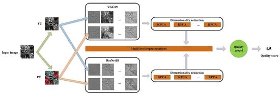
The proposed MLPSIE uses the two deep learning networks, ResNet18 [31] and VGG19 [32]. However, as it is shown in Section 3.5 (Ablation Tests) the proposed processing of multi-level data allows for obtaining features sensitive to distortions which can be applied to other network pairs or even single architectures, leading to acceptable results. It is worth noticing that the networks are not trained due to the size of the image database and the obtained promising performance of the approach. However, if needed, it is assumed that the released source code of the MLPSIE can be adapted to perform a fine-tuning of the networks to capture image characteristics of a specific problem. The source code is available at http://marosz.kia.prz.edu.pl/MLPSIE.html, accessed on 13 January 2022. As presented in Figure 1 with the block diagram, the PS image composed of the RGB and near-infrared (NIR) bands is used to create the true color (TC) RGB and pseudocolor (PC) NIR + RG inputs to the network pair. Then, high-dimensional network responses at each level are extracted (blue rectangles in the figure) and reduced using the Kernel PCA (KPCA) approach (brown rectangles) [33]. The reduction takes place for concatenated TC and PC information, represented by dashed lines. Finally, the reduced features are concatenated (longer brown block) and used by the quality model obtained with the SVR to predict the quality of the PS image (green circle).

2.1. Network Architectures

In this paper, ResNet18 and Vgg19 architectures are used for the PS IQA. The Visual Geometry Group Network (VGGNet) is a deep learning algorithm with a multi-layered operation [34]. It consists of 16 convolution layers and three fully-connected layers, where 3 × 3 convolutional layers are placed on the top to increase with depth level. In the first two convolutional layers, 64 kernels (3 × 3 filter size) and the same padding are included. In this network architecture, the input is of a fixed size of 224 × 224. The pre-processing is done by the subtraction of the mean value from each pixel and is calculated for the entire training set. Moreover, max-pooling is performed over a 2 × 2 pixel window. In the set of fully connected layers, the first two are of size 4096 and the third layer consists of 1000 channels, while the final layer is a SoftMax function. In ResNet18, to avoid two or three layers containing ReLU and batch normalization, the architecture uses shortcut connections. Additionally, it solves the problem of vanishing gradients which increase the training error with a growing number of layers. The shortcut connections that allow skipping the layers allow for the training of deeper networks. At an early stage, the architecture performs the convolution (7 × 7) and max pooling (3 × 3). As the last layers, the average pooling and fully-connected layer are used [31,35].

2.2. Multi-Level Features

Since networks are designed to work with three-band RGB images and the proposed approach should be able to produce a quality score based on two three-band images, the feature vector extracted from the l-th layer of the n-th network can be written as $V_l^n$, where $l=1,2,\cdots ,L_n$, and $L_n$ is the number of convolutional layers in the network. Hence, multi-level data extracted from the network can be written as $V_n=[V_1^n,V_2^n,\cdots ,V_{L_n}^n]$, and taking into account PC and TC images and both networks used in this study ($n=1$ for ResNet18 and $n=2$ for VGG19), the resulted representation of PS image is $V=[V_1\left(RGB\right),V_1(NIR+RG),V_2\left(RGB\right),V_2(NIR+RG)]$. Note that for example, the first layers of ResNet18 and VGG19 contain 802816 and 3211264 values, respectively. Therefore, to create quality models without discarding important information that is stored at various levels of the networks, in this study, each layer is processed independently by the KPCA to produce a compact and distinctive quality-aware vector. Since two networks of each deep learning backbone are used to extract features from the TC and PC images, they are concatenated together. Finally, the vector $\mathcal{V}=$$\left[KPCA\right([V_1^1\left(RGB\right),V_1^1(NIR+RG)],\cdots ,KPCA\left([V_{L_1}^1\left(RGB\right),V_{L_1}^1(NIR+RG)]\right),KPCA([V_1^2\left(RGB\right),V_1^2(NIR+RG)],\cdots ,$

$KPCA\left([V_{L_2}^2\left(RGB\right),V_{L_2}^2(NIR+RG)]\right)]$.

The KPCA implements classical PCA but it can be also used for non-linear problems or problems in which the number of components should be determined automatically [33,36]. It is employed in this work as it provides satisfactory output with ease of implementation.

Once feature vectors characterizing training images are obtained with the proposed method, a quality model can be trained. Here, the SVR is used due to its popularity and dominant position among similar solutions in the IQA literature [28]. The used $\epsilon$-SVR maps feature vector for an image ($\mathcal{V}$) into its subjective score (S). Given the training data $(\mathcal{V},S)$, where $\mathcal{V}$ denotes feature vectors of M training images (${\mathcal{V}}_1,{\mathcal{V}}_2,\cdots ,{\mathcal{V}}_M$) and S contains their subjective scores, i.e., Differential Mean Opinion Scores (DMOS), ($S_1,S_2,\cdots ,S_M$), a function $\mathfrak{f}\left(\mathcal{V}\right)=\langle$$\omega$, $\mathcal{V}$〉 + b is determined in which $\langle ·,·\rangle$, $\omega$, and b, are the inner product, weight vector, and a bias parameter, respectively. Once the slack variables ${\xi }_m$ and ${\xi }_m^{*}$ are introduced, the $\omega$ and b are the solution of the following optimization problem:

$$\begin{array}{cc}& \mathrm{minimize}\frac{1}{2}{∥\omega ∥}^2+C\sum _{m=1}^M({\xi }_m+{\xi }_m^{*})\hfill \\ \hfill & subjectto\left\{\begin{array}{c}〈\omega ,{\mathcal{V}}_m〉-(S_m-b)\le \epsilon +{\xi }_m\hfill \\ S_n-b-〈\omega ,{\mathcal{V}}_m〉\le \epsilon +{\xi }_m^{*}\hfill \\ {\xi }_m,{\xi }_m^{*}\ge 0,\hfill \end{array}\right.\hfill \end{array}$$

(1)

where C balances $\omega$, ${\xi }_m$, and ${\xi }_m^{*}$. The $\omega ={\sum }_{m=1}^M{t}_m{V}_m$, where $t_m$ is a combination coefficient. The $\mathcal{V}$ is mapped into $\Phi \left(\mathcal{V}\right)$,

$$\begin{array}{cc}\hfill \mathfrak{f}\left(\mathcal{V}\right)=& 〈\sum _{m=1}^M{t}_m\Phi \left({\mathcal{V}}_m\right),\Phi \left(\mathcal{V}\right)〉+b\hfill \\ \hfill =& \sum _{m=1}^M{t}_m〈\Phi \left({\mathcal{V}}_m\right),\Phi \left(\mathcal{V}\right)〉+b.\hfill \end{array}$$

(2)

For the RBF kernel,

$$\begin{array}{c}\hfill \mathfrak{f}\left(\mathcal{V}\right)=\sum _{m=1}^M{t}_{m}exp(-\gamma (|{\mathcal{V}}_m-{V\left|\right)}^2)+b,\end{array}$$

(3)

where, the $\gamma$ is the precision parameter.

3. Results

3.1. Ps Image Database

In experiments, an image database originated from the IKONOS satellite images and assessed by human observers in the study of Agudelo-Medina et al. [1] is used. In that work, five regions of interest were used. However, this study effectively uses only four of them since in its shared version only full sets of their images are associated with subjective scores. It is worth noticing that this dataset is the largest image collection of PS images assessed by human observers and can be employed to thoroughly compare PS methods as well as techniques used for their assessment. The dataset contains 171 PS images (TC and PC pairs) obtained from four reference images using six PS methods (IHS [4]—28, BDSD [37]—24, PCA [3]—28, MTF-GLP-CBD [38]—28, HPF [5]—28, and ATWT-M2 [39]—31) and one interpolation method (EXT [40]—4). Additionally, images are distorted with blur and additive white Gaussian noise [1]. The following regions are considered: Coliseum, Road, Urban, River, and Villa. However, due to low number of released Villa images, they are only used in the training subsets. Each region of 256 × 256 × 4 pixels for MS and 1024 × 1024 pixels for PAN was extracted from the image of the city of Rome. Subjective scores are assigned to the TC and PC images. Hence, to use both values for the training of a method on the PS images, their geometric mean is employed (DMOS-GM). The dataset also contains four undistorted PS images of the extracted IKONOS scenes. Exemplary undistorted and blurred TC and PC images of the IKONOS Roma Urban scene are presented in Figure 2.

3.2. Experimental Protocol

The proposed method is evaluated using a typical protocol used for the comparison of IQA approaches. In the protocol, four evaluation criteria are used: Spearman Rank-order Correlation Coefficient (SRCC), Kendall Rank Order Correlation Coefficient (KRCC), Pearson Linear Correlation Coefficient (PLCC), and Root Mean Square Error (RMSE) [41]. The criteria are calculated between predicted scores returned by a method and DMOS-GM. The higher correlation value and lower RMSE denote a better IQA method. It is worth noticing that the RMSE is often used to evaluate quality PS images, employed as an FR method. However, similarly to other IQA studies, it is used in this work to assess prediction accuracy, together with the PLCC. The SRCC and KRCC evaluate prediction monotonicity [41]. Since the MLPSIE requires training, images from the database are divided into training and testing subsets, and the evaluation criteria are reported as medians calculated for the testing subsets. Consequently, the methods that do not require training are only using test images in the experiments. Various experimental scenarios are considered, taking into account the number of reference images, random division of examples, or distortion types. To support the results, statistical significance tests are reported as well as a discussion on the capability of the best methods to sort outputs of PS approaches in comparison to quality scores of human observers (DMOS-GM).

3.3. Comparison of Nr Methods

The proposed method is experimentally compared with 17 state-of-the-art approaches with available source codes: BRISQUE [26], CurveletQA [42], FRIQUEE [43], GMLOG [44], GWH-GLBP [24], NFERM [27], NOREQI [45], Oracle [46], SCORER [47], SISBLIM [48], BPRI [23], SINDEX [49], dipIQ [50], Blinder [28], $Q_{oa}$ [1], ERGAS [20], and R50GR18 [29]. Since the $Q_{oa}$ is reported to outperform other PS IQA methods, the comparison covers also the FR ERGAS technique that yields promising results in many experiments. The $Q_{oa}$ is a training-based technique, similarly to MLPSIE, which allows for the comparison of the IQA capabilities of features used in both solutions. Among the remaining methods, R50GR15, dipIQ, and BLINDER are deep learning-based measures. However, only implementations of the R50GR15 and BLINDER can be trained while the dipIQ does not offer such functionality. Hence, it is evaluated on the testing images as other methods that do not require such a step (CurveletQA, BPRI, SINDEX, and ERGAS). All approaches that originate from the IQA of natural or medical images extract features from PC and TC images and after their concatenation appropriate regression models are trained to provide a quality prediction. Hence, in this work, popular IQA methods are adapted to the PS IQA. In the cases of CurveletQA, BPRI, SINDEX, and ERGAS, TC and PC images are evaluated and their scores are averaged to provide overall quality scores for PS images. The approaches are run in Matlab R2021a, Windows 10, on a PC with an i9-12900k CPU, 128 GB RAM, and an RTX 3090 graphic card. In the MLPSIE, the GPU extracts the features from the networks, while the CPU determines the multi-level image representations and predicts image quality. The SVR parameters of relevant methods are obtained using grid search.

Since there are four base PS scenes, i.e., Coliseum, Road, Urban, and River, in the first experimental scenario, all images that belong to one scene are used for testing while the remaining images train the NR methods. The median evaluation criteria from four tests are reported in

Table 1. Comparison of performance of approaches for different scenes.

Method	SRCC	KRCC	PLCC	RMSE
BRISQUE	0.9007	0.7473	0.9655	1.9523
CurveletQA	0.9443	0.8098	0.9720	1.6473
FRIQUEE	0.8183	0.6336	0.9124	3.2830
GMLOG	0.9200	0.7698	0.9653	2.1162
GWH-GLBP	0.8766	0.7121	0.9377	2.7140
NFERM	0.9373	0.7981	0.9698	1.8099
NOREQI	0.8779	0.7110	0.9511	2.5011
Oracle	0.7882	0.5879	0.4137	7.1081
SCORER	0.7955	0.5857	0.7728	4.6842
SISBLIM	0.8026	0.6135	0.8808	3.8421
BPRI	0.4599	0.2957	0.6107	5.8090
SINDEX	0.8749	0.6848	0.9118	3.1256
dipIQ	0.6204	0.4762	0.6821	5.6095
Blinder	0.9115	0.7647	0.9650	1.8550
R50GR18	0.8003	0.6257	0.8136	4.0225
$Q_{oa}$ *	0.8971	0.7307	0.9381	2.7947
ERGAS *°	0.9265	0.7796	0.9658	1.9560
MLPSIE *	0.9548	0.8295	0.9803	1.5797

Note: Three best results for each criterion are written in bold; Approach with ‘*’ is designed for the PS IQA, while ° denotes a FR-IQA method.

. As presented, the introduced MLPSIE outperforms other approaches by a large margin. It is followed by CurvletQA and NFERM. Interestingly, the CurvletQA does not require training which can be seen as an additional advantage. Taking into account IQA methods designed for the PS images, ERGAS outperforms $Q_{oa}$ for all evaluation criteria and is on par with other deep learning approaches trained on PS images (Blinder and R50GR18).

To provide a more thorough examination, similar to the scenario proposed by Agudelo-Medina et al. [1] along with the dataset, the entire image collection is randomly divided into disjoint training and testing samples (80%:20%), disregarding the scene of origin. The evaluation criteria are reported as the median values resulting from 1000 such divisions. The results for the compared methods can be seen in

Table 2. Comparison of methods using 1000 random database splits into training and testing samples.

Method	SRCC	KRCC	PLCC	RMSE
BRISQUE	0.9646	0.8610	0.9844	1.3989
CurveletQA	0.9092	0.7576	0.9488	2.5022
FRIQUEE	0.8921	0.7255	0.9105	3.2761
GMLOG	0.9326	0.7968	0.9556	2.3363
GWH-GLBP	0.9429	0.8146	0.9564	2.3137
NFERM	0.8946	0.7433	0.9435	2.6367
NOREQI	0.9670	0.8645	0.9826	1.4676
Oracle	0.7385	0.5401	0.6025	6.6669
SCORER	0.7328	0.5259	0.7706	5.0609
SISBLIM	0.6796	0.4866	0.7926	4.7989
BPRI	0.3563	0.2442	0.4792	6.9266
SINDEX	0.7792	0.5936	0.8426	4.2549
dipIQ	0.5568	0.4421	0.6565	5.9519
Blinder	0.9426	0.8075	0.9451	2.5781
R50GR18	0.9610	0.8431	0.9693	1.9243
$Q_{oa}$ *	0.9688	0.8681	0.9823	1.4568
ERGAS *°	0.6321	0.4688	0.7482	5.2766
MLPSIE *	0.9749	0.8895	0.9878	1.2359

Note: Three best results for each criterion are written in bold. Approach with ‘*’ is designed for the PS IQA, while ° denotes a FR-IQA method.

. In this scenario, the MLPSIE is the leading technique, with $Q_{oa}$ as the second approach, followed by NOREQI and BRISQUE. This experiment favors methods with powerful features and the capability of creating a quality model. Hence, a simpler ERGAS or deep learning model with pre-trained implementation (dipIQ) obtain inferior results in these tests. To provide additional insight and test whether the indicated differences among results are statistically significant, the Wilcoxon rank-sum test is conducted. This test is considered with a 5% significance level and measures the equivalence of the median value of the samples [51]. In the experiment, a method with a significantly higher SRCC median obtained a score of “1”, the worse “−1”, and indistinguishable “0”. Finally, the results are added to highlight the best approaches (Figure 3). As presented, the statistical significance tests confirm the results shown in Table 2, indicating the best performance of the MLPSIE and promising results for $Q_{oa}$.

The third experimental scenario considers the division of images based on distortion types, i.e., using images affected by two distortion types for training and the remaining distortion for testing. The results reported in

Table 3. Comparison of approaches considering different distortion types.

	UD				BLR				AWGN
Method	SRCC	KRCC	PLCC	RMSE	SRCC	KRCC	PLCC	RMSE	SRCC	KRCC	PLCC	RMSE
BRISQUE	0.9217	0.7619	0.9796	2.3142	0.8760	0.7062	0.9008	2.3757	0.7162	0.5321	0.8245	3.2687
CurveletQA	0.9398	0.8042	0.9787	2.3672	0.7885	0.5992	0.8490	2.8896	0.4229	0.3005	0.4579	5.1348
FRIQUEE	0.8331	0.6402	0.8953	5.1334	0.7508	0.5541	0.8179	3.1469	0.7809	0.6049	0.8799	2.7445
GMLOG	0.8610	0.7143	0.9640	3.0649	0.8610	0.6724	0.8913	2.4798	0.6262	0.4476	0.7821	3.6134
GWH-GLBP	0.9414	0.7989	0.9826	2.1427	0.7388	0.5445	0.8284	3.0633	0.4497	0.3130	0.5005	5.0004
NFERM	0.9119	0.7566	0.9649	3.0271	0.8203	0.6370	0.8559	2.8283	0.7691	0.5790	0.8584	2.9625
NOREQI	0.9562	0.8413	0.9847	2.0071	0.6737	0.4897	0.7672	3.5079	0.4743	0.3419	0.5609	4.7816
Oracle	0.5534	0.3810	0.4637	10.4433	0.5824	0.4196	0.6402	4.4801	0.4453	0.3492	0.1295	5.7758
SCORER	0.7203	0.5397	0.8650	5.7804	0.5395	0.4197	0.3034	5.2115	0.6417	0.4563	0.7331	3.9340
SISBLIM	0.6273	0.5026	0.9216	4.4724	0.7201	0.5155	0.7963	3.3087	0.4966	0.2887	0.6241	4.5131
BPRI	0.7493	0.5291	0.8227	6.5507	0.3381	0.2306	0.3901	5.0361	0.2397	0.1541	0.3680	5.3705
SINDEX	0.6678	0.5238	0.8563	5.9500	0.8389	0.6539	0.8465	2.9120	0.7285	0.5290	0.7894	3.5453
dipIQ	0.1779	0.1429	0.8000	6.9126	0.8445	0.6628	0.8777	2.6213	0.2110	0.1886	0.6949	4.1536
Blinder	0.9294	0.7778	0.9623	3.1339	0.7914	0.6072	0.8347	3.0119	0.8045	0.6369	0.8974	2.5483
R50GR18	0.9223	0.7884	0.9818	2.1880	0.7931	0.6129	0.8669	2.7264	0.7116	0.5290	0.7751	3.6495
$Q_{oa}$ *	0.9502	0.8307	0.9765	2.4809	0.8353	0.6636	0.8688	2.7112	0.7207	0.5266	0.8198	3.3079
ERGAS *°	0.5742	0.4286	0.8348	6.3432	0.5026	0.3561	0.6305	4.2450	0.3960	0.2838	0.6227	4.5193
MLPSIE *	0.9425	0.8307	0.9876	1.8124	0.9393	0.7891	0.9488	1.7280	0.7176	0.5313	0.7877	3.5586

Note: Three best results for each criterion are written in bold. Approach with ‘*’ is designed for the PS IQA, while ° denotes a FR-IQA method.

evidence that MLPSIE is among the three best methods in terms of evaluation criteria for undistorted and blurred images. However, its performance for images distorted with Additive White Gaussian Noise (AWGN) is on par with $Q_{oa}$, behind FRIQUEE, Blinder, or NFERM which by design take into account this distortion type, since it is common in natural images.

3.4. Computational Complexity

Table 4. Run-time comparison.

Method	Time(s)
BRISQUE	0.0057
CurveletQA	0.2457
FRIQUEE	1.7476
GMLOG	0.0053
GWH-GLBP	0.0076
NFERM	2.7032
NOREQI	0.0266
Oracle	0.0722
SCORER	0.0721
SISBLIM	0.1563
BPRI	0.1096
SINDEX	0.0048
dipIQ	0.7501
Blinder	0.6605
R50GR18	0.0079
$Q_{oa}$	0.2898
ERGAS	0.0006
MLPSIE	0.7117

shows the computational complexity measured in terms of the average running time needed for image quality assessment of an image in the database. It can be seen that the MLPSIE is of moderate complexity. The most computationally demanding step in MLPSIE is associated with dimensionality reduction. Note that some of its steps can be performed in parallel to further reduce its computation time. In this experiment, ERGAS is the leading technique, followed by SINDEX or GMLOG. However, despite shorter running times, their IQA efficiency is far behind the proposed approach.

3.5. Ablation Tests

Since in the MLPSIE the KPCA reduces the high-dimensional vectors, the influence of the dimensionality of the resulted feature vector on the performance of the method should be examined. Therefore, the experiment in which PS images are randomly split into training and testing samples 1000 times (see Table 2) is conducted with the dimensionality of vectors for networks’ layers ranging from 5 to 20 with the step of 5. As reported in Figure 4, the performance of the MLPSIE is stable for different values, and the employed dimensionality of 15 seems a reasonable choice.

The same experiment is also employed to show the distinctiveness of convolutional layers in exemplary network architecture. As presented in Figure 5 and Figure 6, most data extracted from layers and reduced by the KPCA is of high importance for the performance of the MLPSIE. The layers with lower SRCC values are likely to be appropriately weighted by the SVR while training the model. Nevertheless, even with single short vectors for layers, the method outperforms many compared techniques (cmp. Table 2). The usage of both networks in the fusion of their such multi-level image representations is responsible for their outstanding performance.

Since the MLPSIE uses two networks, their complementarity should be compared with those of other network alternatives. Therefore, the experiment with random dataset division is performed considering single networks of reasonably low complexity (VGG19, ResNet18, Alexnet, and SqueezeNet) and their combinations. As shown in

Table 5. Comparison of the performance of single and fused networks.

Method	SRCC	KRCC	PLCC	RMSE
VGG19	0.9742	0.8859	0.9852	1.3420
ResNet18	0.9759	0.8877	0.9860	1.2944
AlexNet	0.9697	0.8681	0.9779	1.6430
SqueezeNet	0.9728	0.8824	0.9863	1.3099
AlexNet + ResNet18	0.9746	0.8859	0.9866	1.2839
AlexNet + SqueezeNet	0.9740	0.8859	0.9866	1.2859
MLPSIE (ResNet18 + VGG19)	0.9749	0.8895	0.9878	1.2359

, the employed fusion of the VGG19 and ResNet18 is the most beneficial, in terms of almost all evaluation criteria. However, other network pairs or even single networks also exhibit promising performance. Interestingly, as the networks represent different approaches to deep-learning-based image processing and offer different features, their results are similar, justifying the introduced in this work way of creating and using multi-level image representations as reduced high-dimensional feature vectors extracted from the network layers. Such representations, disregarding the difference in architectures of deep-learning methods that are used to extract features, lead to superior results when compared with other IQA approaches used for the quality prediction of PS images.

The employed channel configuration in MLPSIE assumes that a PS image is transformed into PC and TC image pair, each characterized by three channels since the considered network architectures are devoted to processing RGB images. The used configuration is proposed by Alparone et al. [52] and used in subjective tests with human observers in the work of Agudelo-Medina et al. [1]. However, as presented in

Table 6. Influence of input channel configuration on the quality prediction performance of the MLPSIE. The pair (RGB, NIR + RG) is the default MLPSIE input configuration.

Channel Config.	SRCC	KRCC	PLCC	RMSE
RGB, NIR + RG	0.9749	0.8895	0.9878	1.2359
RGB, NIR + GB	0.9756	0.8895	0.9878	1.2273
RGB, NIR + RB	0.9756	0.8895	0.9879	1.2278
RGB, NIR + NIR + NIR	0.9743	0.8859	0.9871	1.2503

, the MLPSIE can be successfully used with other channel configurations. Here, the combination of the NIR channel with any of two RGB components provides promising results, while creating input composed of three copies of the NIR channel decreases the performance. Consequently, it can be assumed that the quality assessment of images that contain more than channels would be possible once the RGB components are mixed with non-RGB channels of such an image. This would also require the addition of more VGG19 and ResNet18 pairs. The promising results obtained for different combinations of channels, as well as various deep learning backbones (Table 5), allow assuming that the proposed would be suitable, directly or after adaptation and fine-tuning, for applications that require the processing of more channels or involve a fusion of multi-sensor data [53,54].

To show the capability of obtained multi-level image representations to distinguish images of different quality, two-dimensional t-SNE embeddings [55] of features are shown in Figure 7. The figure contains multi-level image representations of images in the dataset for separate (Figure 7b,c) and jointly (Figure 7a) considered networks. To facilitate the visualization with a limited palette of colors, the DMOS-GM scores are scaled. Presented scatter plots for all networks evidence that features allow for the distinction of images that belong to different locations (Coliseum, Road, Urban, and River). At this point in the image processing pipeline, image quality is not considered in the method, since the SVR responsible for the quality prediction is using these features. Hence, the clusters of images of similar quality, reflected by dots of the same or close color in the plots, confirm that the multi-level image representations are sensitive to image distortions and can be used for quality prediction. The t-SNE embeddings for the ResNet and VGG18 are different, and despite irregular cluster boundaries, in most cases, they can be easily differentiated. For the comparison, feature vectors of well-performing $Q_{oa}$ and BRISQUE are also presented. As reported, they have difficulties in clustering images of similar quality. However, in the visualization for the $Q_{oa}$, image clusters of different quality are better distinguished than it can be seen for the BRISQUE.

3.6. Ranking of Ps Methods

Previous tests consider large data quantities to determine the general performance of the methods. However, to support such tests, the ability of the best approaches to select the best PS method and rank their outputs similarly to human observers is also considered. In

Table 7. Subjective (DMOS-GM) and objective scores for IKONOS Rome Urban scene. The lower part of the table contains precedence images produced by PS methods.

	MLPSIE	Blinder	${\mathit{Q}}_{\mathbf{OA}}$	ERGAS	DMOS-GM
PCA	51.69	54.22	47.40	27.16	38.90
MTF-GLP-CBD	53.28	54.21	48.00	26.91	39.84
BDSD	53.1	54.13	49.08	27.34	39.93
IHS	51.96	54.24	49.41	26.12	40.69
HPF	54.55	54.96	51.33	34.70	49.84
ATWT-M2	57.82	55.83	49.81	45.74	60.21
EXP	63.02	56.64	58.97	55.40	71.38
PCA	PCA	BDSD	PCA	IHS
MTF-GLP-CBD	IHS	MTF-GLP-CBD	BDSD	MTF-GLP-CBD
BDSD	BDSD	PCA	ATWT-M2	PCA
IHS	MTF-GLP-CBD	IHS	IHS	BDSD
HPF	HPF	HPF	MTF-GLP-CBD	HPF
ATWT-M2	ATWT-M2	ATWT-M2	HPF	ATWT-M2
EXP	EXP	EXP	EXP	EXP
Number of scores consistent with DMOS	5	5	3	4

,

Table 8. Subjective (DMOS-GM) and objective scores for IKONOS Rome Road scene. The lower part of the table contains precedence images produced by PS methods.

	MLPSIE	Blinder	${\mathit{Q}}_{\mathbf{OA}}$	ERGAS	DMOS-GM
IHS	54.48	56.46	53.14	26.67	31.97
BDSD	55.06	55.56	49.04	25.93	32.53
PCA	54.09	55.92	53.01	27.89	33.19
MTF-GLP-CBD	55.44	55.73	48.97	25.78	35.50
HPF	56.89	56.36	55.36	32.06	42.37
ATWT-M2	60.31	57.45	60.97	42.40	53.83
EXP	64.47	58.13	66.90	52.90	64.98
IHS	PCA	BDSD	MTF-GLP-CBD	MTF-GLP-CBD
BDSD	IHS	MTF-GLP-CBD	BDSD	BDSD
PCA	BDSD	PCA	PCA	IHS
MTF-GLP-CBD	MTF-GLP-CBD	HPF	IHS	PCA
HPF	HPF	IHS	HPF	HPF
ATWT-M2	ATWT-M2	ATWT-M2	ATWT-M2	ATWT-M2
EXP	EXP	EXP	EXP	EXP
Number of scores consistent with DMOS	4	3	5	4

,

Table 9. Subjective (DMOS-GM) and objective scores for IKONOS Rome River scene. The lower part of the table contains precedence images produced by PS methods.

	MLPSIE	Blinder	${\mathit{Q}}_{\mathbf{OA}}$	ERGAS	DMOS-GM
PCA	55.36	53.95	34.89	25.14	40.14
BDSD	56.19	53.66	38.43	24.27	40.37
IHS	55.41	54.25	33.36	25.08	40.63
MTF-GLP-CBD	56.28	53.78	35.57	24.87	41.83
HPF	57.89	54.74	42.93	33.62	48.82
ATWT-M2	61.07	56.10	46.43	44.78	56.96
EXP	64.66	56.62	59.31	53.23	68.50
PCA	PCA	BDSD	IHS	BDSD
BDSD	IHS	MTF-GLP-CBD	PCA	MTF-GLP-CBD
IHS	BDSD	PCA	MTF-GLP-CBD	IHS
MTF-GLP-CBD	MTF-GLP-CBD	IHS	BDSD	PCA
HPF	HPF	HPF	HPF	HPF
ATWT-M2	ATWT-M2	ATWT-M2	ATWT-M2	ATWT-M2
EXP	EXP	EXP	EXP	EXP
Number of scores consistent with DMOS	5	3	3	4

and

Table 10. Subjective (DMOS-GM) and objective scores for IKONOS Rome Coliseum scene. The lower part of the table contains precedence images produced by PS methods.

	MLPSIE	Blinder	${\mathit{Q}}_{\mathbf{OA}}$	ERGAS	DMOS-GM
BDSD	60.43	55.99	49.29	35.33	34.07
PCA	59.17	56.54	56.30	47.13	34.26
IHS	59.70	56.67	53.10	37.25	34.74
MTF-GLP-CBD	60.64	56.06	51.64	37.29	34.81
HPF	61.28	57.09	56.50	40.35	44.65
ATWT-M2	63.64	58.47	60.34	50.00	53.64
EXP	66.82	59.16	63.67	56.96	62.91
BDSD	PCA	BDSD	BDSD	BDSD
PCA	IHS	MTF-GLP-CBD	MTF-GLP-CBD	IHS
IHS	BDSD	PCA	IHS	MTF-GLP-CBD
MTF-GLP-CBD	MTF-GLP-CBD	IHS	PCA	HPF
HPF	HPF	HPF	HPF	PCA
ATWT-M2	ATWT-M2	ATWT-M2	ATWT-M2	ATWT-M2
EXP	EXP	EXP	EXP	EXP
Number of scores consistent with DMOS	4	4	5	3

, scores returned by the best methods indicated in previous experiments, as well as subjective scores (DMOS-GM) and the resultant quality precedence are reported. Four distorted images are separately considered in this experiment. Blinder, MLPSIE, and $Q_{oa}$ were trained on three remaining scenes and their distorted equivalents. The precedence of images produced by different PS methods is shown and written in bold to facilitate analysis. The tables also contain the number of consistent scores obtained by IQA methods with subjective scores. It can be seen from tables that the MLPSIE correctly assessed the precedence of images placing them 18 out of 28 times. This test is particularly challenging since many images are similar according to the DMOS scores and their differentiation requires powerful quality-aware features and a quality model. Here, the $Q_{oa}$ is the second-best technique with 16 correctly placed images. The remaining methods, ERGAS and Blinder, were able to determine the correct position of 15 images. Interestingly, the MLPSIE and $Q_{oa}$ determined the best PS image only two times, and all techniques similarly identified the worst images.

To support the analysis, Table 9 is accompanied by TC images for IKONOS Rome River scene (Figure 8), with magnified selected parts of the images.

4. Conclusions

In this paper, a novel NR IQA method is proposed aimed at quality prediction of PS images. In the method, multi-level representations of PS images offered by two deep learning network architectures are employed as quality-aware features to provide a successful quality model. Since the extracted features from the networks are high-dimensional, they are reduced using the KPCA technique in a layer-wise manner, taking into account the joint reduction of information that describes TC and PC images. As the extensive experimental comparison with 17 approaches reveals, the proposed approach outperforms related methods as well as IQA approaches adapted in this work to the PS domain and can be used to rank PS techniques based on the quality of fused images.

Future work will be focused on the combination of deep learning and classical IQA methods for the IQA of PS images. An organization of subjective tests that include outputs of more PS methods compared to using several high-resolution satellite images, such as QuickBird or WorldView, is also considered.

The code of the introduced MLPSIE is available at http://marosz.kia.prz.edu.pl/MLPSIE.html, accessed on 13 January 2022.

References

- Agudelo-Medina, O.A.; Benitez-Restrepo, H.D.; Vivone, G.; Bovik, A. Perceptual Quality Assessment of Pan-Sharpened Images. Remote Sens. 2019, 11, 877. [Google Scholar] [CrossRef] [Green Version]
- Govind, N.R.; Rishikeshan, C.A.; Ramesh, H. Comparison of Different Pan Sharpening Techniques using Landsat 8 Imagery. In Proceedings of the 2019 IEEE 5th International Conference for Convergence in Technology (I2CT), Bombay, India, 29–31 March 2019; pp. 1–4. [Google Scholar] [CrossRef]
- Du, Q.; Gungor, O.; Shan, J. Performance evaluation for pan-sharpening techniques. In Proceedings of the 2005 IEEE International Geoscience and Remote Sensing Symposium (IGARSS), Seoul, Korea, 29–29 July 2005; pp. 4264–4266. [Google Scholar] [CrossRef]
- Tu, T.M.; Huang, P.S.; Hung, C.L.; Chang, C.P. A fast intensity-hue-saturation fusion technique with spectral adjustment for IKONOS imagery. IEEE Geosci. Remote Sens. Lett. 2004, 1, 309–312. [Google Scholar] [CrossRef]
- Jat, M.; Garg, P.; Dahiya, S. A comparative study of various pixel based image fusion techniques as applied to an urban environment. Int. J. Image Data Fusion 2013, 4, 197–213. [Google Scholar] [CrossRef]
- Ballester, C.; Caselles, V.; Verdera, J.; Rouge, B. A Variational Model for P+XS Image Fusion. Int. J. Comput. Vis. 2006, 69, 43–58. [Google Scholar] [CrossRef]
- Huang, W.; Xiao, L.; Wei, Z.; Liu, H.; Tang, S. A new pan-sharpening method with deep neural networks. IEEE Geosci. Remote Sens. Lett. 2015, 12, 1037–1041. [Google Scholar] [CrossRef]
- Kau, L.J.; Lee, T.L. An HSV Model-Based Approach for the Sharpening of Color Images. In Proceedings of the 2013 IEEE International Conference on Systems, Man, and Cybernetics, Manchester, UK, 13–16 October 2013; pp. 150–155. [Google Scholar] [CrossRef]
- Jawak, S.D.; Luis, A.J. A Comprehensive Evaluation of PAN-Sharpening Algorithms Coupled with Resampling Methods for Image Synthesis of Very High Resolution Remotely Sensed Satellite Data. Adv. Remote Sens. 2013, 2013, 332–344. [Google Scholar] [CrossRef] [Green Version]
- Jing, L.; Cheng, Q. Two improvement schemes of PAN modulation fusion methods for spectral distortion minimization. Int. J. Remote Sens. 2009, 30, 2119–2131. [Google Scholar] [CrossRef]
- Laben, C.A.; Brower, B.V. Process for Enhancing the Spatial Resolution of Multispectral Imagery Using Pan-Sharpening. U.S. Patent 6,011,875, 4 January 2000. [Google Scholar]
- Alparone, L.; Aiazzi, B.; Baronti, S.; Garzelli, A.; Nencini, F.; Selva, M. Multispectral and Panchromatic Data Fusion Assessment Without Reference. ASPRS J. Photogramm. Eng. Remote Sens. 2008, 74, 193–200. [Google Scholar] [CrossRef] [Green Version]
- Vivone, G.; Dalla Mura, M.; Garzelli, A.; Restaino, R.; Scarpa, G.; Ulfarsson, M.O.; Alparone, L.; Chanussot, J. A New Benchmark Based on Recent Advances in Multispectral Pansharpening: Revisiting Pansharpening With Classical and Emerging Pansharpening Methods. IEEE Geosci. Remote Sens. Mag. 2021, 9, 53–81. [Google Scholar] [CrossRef]
- Khan, M.; Alparone, L.; Chanussot, J. Pansharpening Quality Assessment Using the Modulation Transfer Functions of Instruments. Geosci. Remote Sens. IEEE Trans. 2009, 47, 3880–3891. [Google Scholar] [CrossRef]
- Wang, Z.; Bovik, A.C. A universal image quality index. IEEE Signal Process. Lett. 2002, 9, 81–84. [Google Scholar] [CrossRef]
- Vivone, G.; Alparone, L.; Chanussot, J.; Dalla Mura, M.; Garzelli, A.; Licciardi, G.A.; Restaino, R.; Wald, L. A Critical Comparison Among Pansharpening Algorithms. IEEE Trans. Geosci. Remote Sens. 2015, 53, 2565–2586. [Google Scholar] [CrossRef]
- Alcaras, E.; Parente, C.; Vallario, A. Automation of Pan-Sharpening Methods for Pleiades Images Using GIS Basic Functions. Remote Sens. 2021, 13, 1550. [Google Scholar] [CrossRef]
- Zhang, Y.; Atkinson, P.M.; Ling, F.; Foody, G.M.; Wang, Q.; Ge, Y.; Li, X.; Du, Y. Object-Based Area-to-Point Regression Kriging for Pansharpening. IEEE Trans. Geosci. Remote Sens. 2021, 59, 8599–8614. [Google Scholar] [CrossRef]
- Sarp, G. Spectral and spatial quality analysis of pan-sharpening algorithms: A case study in Istanbul. Eur. J. Remote Sens. 2014, 47, 19–28. [Google Scholar] [CrossRef] [Green Version]
- Kim, M.; Holt, J.; Madden, M. Comparison of Global- and Local-scale Pansharpening for Rapid Assessment of Humanitarian Emergencies. Photogramm. Eng. Remote Sens. 2011, 77, 51–63. [Google Scholar] [CrossRef]
- Javan, F.D.; Samadzadegan, F.; Reinartz, P. Spatial Quality Assessment of Pan-Sharpened High Resolution Satellite Imagery Based on an Automatically Estimated Edge Based Metric. Remote Sens. 2013, 5, 6539–6559. [Google Scholar] [CrossRef]
- Alimuddin, I.; Sumantyo, J.T.S.; Kuze, H. Assessment of pan-sharpening methods applied to image fusion of remotely sensed multi-band data. Int. J. Appl. Earth Obs. Geoinf. 2012, 18, 165–175. [Google Scholar]
- Min, X.; Gu, K.; Zhai, G.; Liu, J.; Yang, X.; Chen, C.W. Blind quality assessment based on pseudo-reference image. IEEE Trans. Multimed. 2017, 20, 2049–2062. [Google Scholar] [CrossRef]
- Li, Q.; Lin, W.; Fang, Y. No-Reference Quality Assessment for Multiply-Distorted Images in Gradient Domain. IEEE Signal Process. Lett. 2016, 23, 541–545. [Google Scholar] [CrossRef]
- Ma, K.; Liu, W.; Zhang, K.; Duanmu, Z.; Wang, Z.; Zuo, W. End-to-End Blind Image Quality Assessment Using Deep Neural Networks. IEEE Trans. Image Process. 2018, 27, 1202–1213. [Google Scholar] [CrossRef] [PubMed]
- Mittal, A.; Moorthy, A.K.; Bovik, A.C. No-Reference Image Quality Assessment in the Spatial Domain. IEEE Trans. Image Process. 2012, 21, 4695–4708. [Google Scholar] [CrossRef] [PubMed]
- Gu, K.; Lin, W.; Zhai, G.; Yang, X.; Zhang, W.; Chen, C.W. No-reference quality metric of contrast-distorted images based on information maximization. IEEE Trans. Cybern. 2016, 47, 4559–4565. [Google Scholar] [CrossRef]
- Gao, F.; Yu, J.; Zhu, S.; Huang, Q.; Tian, Q. Blind image quality prediction by exploiting multi-level deep representations. Pattern Recognit. 2018, 81, 432–442. [Google Scholar] [CrossRef]
- Stępień, I.; Obuchowicz, R.; Piórkowski, A.; Oszust, M. Fusion of Deep Convolutional Neural Networks for No-Reference Magnetic Resonance Image Quality Assessment. Sensors 2021, 21, 1043. [Google Scholar] [CrossRef]
- Ieremeiev, O.; Lukin, V.; Okarma, K.; Egiazarian, K. Full-Reference Quality Metric Based on Neural Network to Assess the Visual Quality of Remote Sensing Images. Remote Sens. 2020, 12, 2349. [Google Scholar] [CrossRef]
- Napoletano, P.; Piccoli, F.; Schettini, R. Anomaly Detection in Nanofibrous Materials by CNN-Based Self-Similarity. Sensors 2018, 18, 209. [Google Scholar] [CrossRef] [Green Version]
- Pires de Lima, R.; Marfurt, K. Convolutional Neural Network for Remote-Sensing Scene Classification: Transfer Learning Analysis. Remote Sens. 2020, 12, 86. [Google Scholar] [CrossRef] [Green Version]
- Wang, W.; Zhang, M.; Wang, D.; Jiang, Y. Kernel PCA feature extraction and the SVM classification algorithm for multiple-status, through-wall, human being detection. EURASIP J. Wirel. Commun. Netw. 2017, 2017, 151. [Google Scholar] [CrossRef] [Green Version]
- Kemker, R.; Salvaggio, C.; Kanan, C. Algorithms for Semantic Segmentation of Multispectral Remote Sensing Imagery using Deep Learning. arXiv 2018, arXiv:1703.06452. [Google Scholar] [CrossRef] [Green Version]
- Xie, S.; Girshick, R.; Dollár, P.; Tu, Z.; He, K. Aggregated Residual Transformations for Deep Neural Networks. arXiv 2017, arXiv:1611.05431. [Google Scholar]
- Licciardi, G.; Vivone, G.; Dalla Mura, M.; Restaino, R.; Chanussot, J. Multi-resolution analysis techniques and nonlinear PCA for hybrid pansharpening applications. Multidimens. Syst. Signal Process. 2016, 27, 807–830. [Google Scholar] [CrossRef]
- Vivone, G. Robust Band-Dependent Spatial-Detail Approaches for Panchromatic Sharpening. IEEE Trans. Geosci. Remote. Sens. 2019, 9, 6421–6433. [Google Scholar] [CrossRef]
- Jiao, J.; Wu, L.; Qian, K. A Segmentation-Cooperated Pansharpening Method Using Local Adaptive Spectral Modulation. Electronics 2019, 8, 685. [Google Scholar] [CrossRef] [Green Version]
- Li, J.; Hu, Q.; Ai, M. Multispectral and panchromatic image fusion based on spatial consistency. Int. J. Remote Sens. 2018, 39, 1017–1041. [Google Scholar] [CrossRef]
- Aiazzi, B.; Alparone, L.; Baronti, S.; Garzelli, A. Context-driven fusion of high spatial and spectral resolution images based on oversampled multiresolution analysis. IEEE Trans. Geosci. Remote Sens. 2002, 40, 2300–2312. [Google Scholar] [CrossRef]
- Sheikh, H.; Sabir, M.; Bovik, A. A Statistical Evaluation of Recent Full Reference Image Quality Assessment Algorithms. IEEE Trans. Image Process. 2006, 15, 3440–3451. [Google Scholar] [CrossRef]
- Ahmed, I.T.; Der, C.S. Enhancement of no-reference image quality assessment for contrast-distorted images using natural scene statistics features in Curvelet domain. In Proceedings of the 2017 7th IEEE International Conference on System Engineering and Technology (ICSET), Shah Alam, Malaysia, 2–3 October 2017; pp. 128–133. [Google Scholar] [CrossRef]
- Ghadiyaram, D.; Bovik, A.C. Perceptual Quality Prediction on Authentically Distorted Images Using a Bag of Features Approach. arXiv 2016, arXiv:1609.04757. [Google Scholar] [CrossRef]
- Abdul, R. New Learning Frameworks for Blind Image Quality Assessment Model. Ph.D. Thesis, University of Sheffield, Sheffield, UK, 2018. [Google Scholar]
- Oszust, M. No-reference image quality assessment using image statistics and robust feature descriptors. IEEE Signal Process. Lett. 2017, 24, 1656–1660. [Google Scholar] [CrossRef]
- Babonneau, F.; Beltran, C.; Haurie, A.; Tadonki, C.; Vial, J.P. Proximal-ACCPM: A versatile oracle based optimisation method. In Optimisation, Econometric and Financial Analysis; Springer: Berlin/Heidelberg, Germany, 2007; pp. 67–89. [Google Scholar] [CrossRef]
- Liu, T.J.; Liu, K.H. No-Reference Image Quality Assessment by Wide-Perceptual-Domain Scorer Ensemble Method. IEEE Trans. Image Process. 2018, 27, 1138–1151. [Google Scholar] [CrossRef]
- Gu, K.; Zhai, G.; Yang, X.; Zhang, W. Hybrid no-reference quality metric for singly and multiply distorted images. IEEE Trans. Broadcast. 2014, 60, 555–567. [Google Scholar] [CrossRef]
- Leclaire, A.; Moisan, L. No-reference image quality assessment and blind deblurring with sharpness metrics exploiting fourier phase information. J. Math. Imaging Vis. 2015, 52, 145–172. [Google Scholar] [CrossRef] [Green Version]
- Ma, K.; Liu, W.; Liu, T.; Wang, Z.; Tao, D. dipIQ: Blind image quality assessment by learning-to-rank discriminable image pairs. IEEE Trans. Image Process. 2017, 26, 3951–3964. [Google Scholar] [CrossRef] [PubMed] [Green Version]
- De Barros, R.S.M.; Hidalgo, J.I.G.; de Lima Cabral, D.R. Wilcoxon rank sum test drift detector. Neurocomputing 2018, 275, 1954–1963. [Google Scholar] [CrossRef]
- Alparone, L.; Wald, L.; Chanussot, J.; Thomas, C.; Gamba, P.; Bruce, L.M. Comparison of pansharpening algorithms: Outcome of the 2006 GRS-S data-fusion contest. IEEE Trans. Geosci. Remote Sens. 2007, 45, 3012–3021. [Google Scholar] [CrossRef] [Green Version]
- Ehlers, M.; Klonus, S.; Astrand, P.J.; Rosso, P. Multi-sensor image fusion for pansharpening in remote sensing. Int. J. Image Data Fusion 2010, 1, 25–45. [Google Scholar] [CrossRef]
- Kizel, F.; Benediktsson, J.A. Spatially Enhanced Spectral Unmixing Through Data Fusion of Spectral and Visible Images from Different Sensors. Remote Sens. 2020, 12, 1255. [Google Scholar] [CrossRef] [Green Version]
- Hinton, G.; Roweis, S. Stochastic Neighbor Embedding. In Proceedings of the 15th International Conference on Neural Information Processing Systems, Vancouver, BC, Canada, 9–14 December 2002; MIT Press: Cambridge, MA, USA, 2002; pp. 857–864. [Google Scholar]
Figure 1.
Block diagram of the method. Features extracted from both networks for the PC and TC images of input PS image (represented by blue rectangles) are reduced using KPCA (brown blocks) and concatenated for quality prediction by the trained SVR (green circle).
Figure 2.
True color (a,c) and pseudo color (b,d) images of undistorted (a,b) and blurred (c,d) IKONOS Roma Urban scene.
Figure 3.
Results of statistical significance tests.
Figure 4.
Median PLCC values for the MLPSIE with different dimensionality of reduced vectors.
Figure 5.
Performance of features in convolutional layers of the ResNet18 network in terms of the SRCC criterion.
Figure 6.
Performance of features in convolutional layers of the VGG19 network in terms of the SRCC criterion.
Figure 7.
Scatter plots with two-dimensional t-SNE embeddings of MLPSIE multi-level features for the PS images of four categories in the dataset (a), VGG19 (b), and ResNet18 (c). Embeddings for the BRISQUE (d) and (e) are also shown. Colors indicate scaled DMOS-GM scores for images.
Figure 8.
TC images obtained with PS methods compared with the reference (Ref) for IKONOS Rome River scene.