
Exploring the Spatiotemporal Coverage of Terrestrial Snow Mass Using a Suite of Satellite Constellation Configurations


1
Civil and Environmental Engineering, University of Maryland, College Park, MD 20742, USA
2
NASA Goddard Space Flight Center, Greenbelt, MD 20771, USA
*
Author to whom correspondence should be addressed.
Remote Sens. 2022, 14(3), 633; https://doi.org/10.3390/rs14030633
Submission received: 5 January 2022
/
Accepted: 24 January 2022
/
Published: 28 January 2022
(This article belongs to the Special Issue Remote Sensing in Snow and Glacier Hydrology)
Abstract
:Terrestrial snow is a vital freshwater resource for more than 1 billion people. Remotely-sensed snow observations can be used to retrieve snow mass or integrated into a snow model estimate; however, optimally leveraging remote sensing observations of snow is challenging. One reason is that no single sensor can accurately measure all types of snow because each type of sensor has its own unique limitations. Another reason is that remote sensing data is inherently discontinuous across time and space, and that the revisit cycle of remote sensing observations may not meet the requirements of a given snow applications. In order to quantify the feasible availability of remotely-sensed observations across space and time, this study simulates the sensor coverage for a suite of hypothetical snow sensors as a function of different orbital configurations and sensor properties. The information gleaned from this analysis coupled with a dynamic snow binary map is used to evaluate the efficiency of a single sensor (or constellation) to observe terrestrial snow on a global scale. The results show the efficacy achievable by different sensors over different snow types. The combination of different orbital and sensor configurations is explored to requirements of remote sensing missions that have 1-day, 3-day, or 30-day repeat intervals. The simulation results suggest that 1100 km, 550 km, and 200 km are the minimum required swath width for a polar-orbiting sensor to meet snow-related applications demanding a 1-day, 3-day, and 30-day repeat cycles, respectively. The results of this paper provide valuable input for the planning of a future global snow mission.

1. Introduction
Snow is an important component of global freshwater storage. It provides freshwater supply for more than 1 billion people [1,2,3]. Snow-covered terrain serves as a natural reservoir that slowly attenuates freshwater runoff during the snow ablation season [4]. Snow albedo also plays an important role in energy balance and climate change. For example, atmospheric warming could reduce the seasonal snow cover and, hence, increase shortwave absorption at the land surface, which could introduce a positive feedback [5].
Snow storage estimation is increasingly important as the virtual reservoir of snow is threatened by global warming and climate change [6,7,8]. Earlier snowmelt due to global warming could exacerbate severe floods and droughts [9,10,11]. As a result, the vulnerability of snow storage has attracted considerable interest from the hydrologic community to monitor the equivalent amount of liquid water contained within the snowpack (a.k.a snow water equivalent or SWE) so that this vital resource may be better managed and preserved.
1.1. Limitations of Existing Spaceborne Snow Products
Spaceborne remote sensing is the only viable technique to detect SWE across the globe in a timely manner [12] when considering the large spatial extent of snow and the difficulties in collecting in-situ measurements over such large regions. Despite the extensive efforts of researchers to provide accurate SWE retrievals, current SWE products using passive microwave (PMW) remote sensing observations still do not meet the accuracy requirements (±15%) needed to support operational decision-making at a continental or global scale [13,14]. One main reason is the knowledge gap in coupling precise physical emission models (i.e., radiative transfer models (RTMs)) of snowpacks to remotely-sensed observations [12].
A general approach for using PMW observations is the spectral polarization difference (SPD) [15] employing the Chang algorithm [16] and its modification for forested areas (Foster 1997); this approach uses PMW spectral difference, i.e., the difference in brightness temperature between two microwave frequency channels. This technique is effective in some regions e.g., dry, shallow snow on flat terrain, but is unable to detect thin snow due to a low signal-to-noise ratio, or accurately retrieve deep snow due to signal saturation, or snow with overlying vegetation due to vegetation attenuation [12,17]. To help overcome the problems of PMW observations across regional or continental scales, some studies have fused satellite data with ground-based snow measurements to better estimate SWE [18,19].
There has never been a dedicated satellite mission for snow mass (SWE) detection. Existing spaceborne sensors used to estimate snow mass have typically been designed for a different purpose [20]. With the above limitations, most operational, stand-alone passive microwave SWE products produced using the spectral difference method are far from optimal. Typically, these products are inconsistent with independent reanalysis data and ground-based measurements from meteorological stations and snow courses [10,21], particularly in deep snow, wet snow, snow in complex terrain, or snow with overlying vegetation [10,17,22].
Analogously, the Moderate Resolution Imaging Spectroradiometer (MODIS), a passive visible and thermal infrared radiometer, was designed to view the spatial extent of snow rather than the mass of snow within that snow-covered extent. Thus, MODIS is limited in skill in terms of snow mass estimation although it does an good job of viewing where snow is found on the ground in the absence of dense forest [9,23]. More recently, active microwave (AMW) synthetic aperture radar (SAR) has been employed for global snow mass detection [24,25], but two issues remain unsolved: one is the limited repeat overpass (relative to Advanced Microwave Scanning Radiometer (AMSR) or MODIS), and the other is that C-band microwave radiation on, e.g., Sentinel-1, is not as sensitive to snow volume scattering as compared to X-band or as skilled in the detection of shallow snow as compared to Ku-band [26,27], although recent studies showed its potential at mapping snow mass in mountainous regions [28]. Suffice it to say that the development of such sensors for purposes other than terrestrial snow mass limits the skill of these sensors in the application to global SWE estimation. As a result, the snow science community is discussing the prospect of a future, dedicated spaceborne snow mission which would be the first of its kind [29,30].
1.2. Limitations of Remote Sensing Snow Techniques
The complexity of snow further confounds the retrieval of snow properties using remotely-sensed observations such that no single technique can work for all types of snow. One significant source of uncertainty in retrieving snow mass comes from the sensitivity of remotely-sensed observations to other snow-related variables, such as snow microstructure (e.g., grain size), snow stratigraphy, the amount of liquid water content coating the snow grains, overlying vegetation, complex topography, and atmospheric and cloud conditions [17]. Microwave radiation, in general, is sensitive to the snow liquid water content (SLWC) such that even a small amount of liquid water in the snowpack greatly alters the dielectric constant and, hence, the emissivity and absorptivity of the snowpack. SLWC, which is relatively large during the melting season, often introduces large uncertainties into SWE retrievals from both PMW and AMW retrievals [31]. Snow density, snow grain size, and snow grain shape are other variables that influence the snow emissivity and scattering characteristics and, as a result, the corresponding electromagnetic response of the snowpack [12]. The variability in these snow characteristics can result in a strong correlation between the PMW signals and snow mass for some years, but not for other years. Additionally, the complex microstructure of a snowpack due to variations in depth hoar, internal ice layering, and vertical heterogeneity increase the spatial and temporal variability of the snowpack [12]. Overlying vegetation further complicates snow remote sensing by attenuating microwave emission from the snowpack, while simultaneously contributing its own signal as measured by the spaceborne radiometer. Findings have shown that PMW SWE retrievals tend to underestimate SWE in forested areas [32]. Complex terrain, such as in mountains, also reduces the efficacy of coarse-resolution sensors, such as PMW radiometers or AMW scatterometers [17,33,34]. All of these uncertainties are exacerbated by the coarse-scale resolution of these measurements that cannot adequately capture the true spatial variability of SWE [35,36]. To overcome this problem, recent studies improved large-scale patterns of snow mass estimation by merging PMW observations with ground-based measurements [19,28].
In the context of spaceborne LiDAR, which is another option for retrieving snow depth and snow mass, a major limitation is the relatively narrow swath width of LiDAR [37] (~10 km) as compared to SAR (~100 km) or PMW radiometry (~1000 km). The individual LiDAR beams typically obtain tracks with widths of 100 meters or less. Using multiple LiDAR beams as part of a sampling strategy, the swath width of a spaceborne LiDAR retrieval is typically around 6 km [38,39]. Furthermore, the optical signal used by a snow LiDAR cannot penetrate optically-thick clouds [40]; hence, the snow under the clouds remains unobserved. LiDAR is an effective tool for retrieving snow depth, but that effectiveness is severely curtailed when considering swath width limitations and cloud attenuation.
In short, no single spaceborne sensor will adequately measure all types of snow under all conditions required for global snow monitoring. Rather, a mixture of observations from different sensors, each with its own strengths and weaknesses, is needed to yield the best estimate of global snow mass [37].
1.3. Snow Mass Mission Trade-Offs
To make global snow mass estimation even more complicated, a future snow mission will face a trade-off between sensor design, spatial resolution, and revisit frequency. For example, a different orbital configuration (largely as a function of inclination angle and satellite altitude) changes the nadir track, which directly influences which portions of the globe are, or are not, observed. Similarly, a wider swath width for a given sensor increases the revisit frequency but likely results in larger errors along the swath periphery due to slant range geometry effects or significant reductions in backscatter, e.g., associated with changes in forward scattering characteristics as the sensor looks increasingly off-nadir [41]. An increase in satellite altitude or changes in orbital parameters could impact the spatial resolution, as well as the frequency with which the globe is viewed. However, both the fine spatial resolution and short revisit interval are of interest in SWE estimation considering the strong spatiotemporal dynamics of the snow [42,43]. Additional concerns about this trade-off include non-uniform distribution of snow cover and diversity of snow types or snow features. The majority of snow occurrence is distributed in the high-latitude or high-altitude regions. Consideration of the different suitable remote sensing techniques to capture the different types of snow, such as tundra, taiga, or ephemeral snow, adds even more complexity to the task of global snow mass estimation.
Given the difficulties listed above, along with the general lack of uptake of PMW estimates of SWE into hydro-meteorology and hydro-climatology applications [35], the research presented here aims to study the efficacy of different orbital configurations and sensor characteristics on snow mass detection from the perspective of maximizing the global snow coverage to be viewed. The goal of this exercise is to facilitate the mission planning process and enhance the future potential of snow remote sensing, e.g., PMW, LiDAR, and SAR.
The first challenge is to link and combine the prediction ability of different satellite orbits and estimation of snow dynamic extent. The sensor’s viewing extent is estimated under various orbital configurations coupled with a snow cover climatology as a function of different snow classes. The goal, hence, is not to quantify global snow mass (which is to be pursued in a follow-up study) but, rather, to explore the different options to quantify snow mass, as well as how best to maximize global coverage (in space and time) en route to estimating global snow mass.
This paper is structured as follows. In Section 2, we introduce the methods to simulate the sensor’s viewing extent given a particular orbital configuration and proposed metrics to analyze the coverage in space and time. We then apply this method to orbital configurations for five different sensors, as well as four different constellations, in Section 3, and then evaluate their effects on snow observability. Section 4 and Section 5 provide a discussion and conclusion on the findings.
2. Methodology
The snow mass detection capability of sensors (and sensor constellations by construct) is limited by the sensors’ viewing extent, the distribution of snow in space and time, and the sensors’ efficacy to specific snow conditions (e.g., ability to retrieve deep snow, wet snow, snow overlain by vegetation). This section introduces the methods to analyze these three factors, including the methodology used to simulate the sensor viewing extent, different scenarios for simulations, application of a dynamic snow mask, and metrics for use in evaluating observation efficacy.
2.1. Simulation of Sensor Viewing Extent
In order to simulate the viewing extent of the single sensor, we use the Trade-space Analysis Tool for Constellations (TAT-C) simulator to explore the ground track of the sensor orbit under different orbital configurations. The module for simulating the sensor orbits in TAT-C has been employed to investigate the nadir position track of a variety of different satellite sensors [44]. The second step in simulating the viewing extent of a single sensor is to adjust the sensor swath width to enhance the hypothetical sensor coverage for this study. Specifically, the satellite viewing extent is generated by extending the ground track in the cross-track direction to a given swath width of interest. The viewing extent simulation is ultimately expressed as a binary map marking the global surface as viewed (or not) in the absence of clouds. The viewing extent simulation is conducted at a 0.01° spatial resolution in this study, and subsequently aggregated in space to match relatively coarse-scale geophysical retrievals in the following analysis. Finally, a realistic cloud mask is convolved with the viewing extent to explore the effects of cloud attenuation on terrestrial snow observability.
2.2. Orbital Configuration and Sensor Type
In short, the orbital configuration mainly depends on satellite altitude and inclination angle. Orbital configuration and swath width determine the repeat cycle of the sensor viewing extent. To represent typical (i.e., polar-orbiting, sun-synchronous) configurations, six different sensors are selected here to represent a range of hypothetical instruments including PMW radiometers, SARs, and LiDARs.
2.2.1. Passive Microwave Radiometer
The first evaluated sensor is an AMSR2-like PMW radiometer [45]. It has a wide swath and relatively high revisit frequency but typically has a coarse spatial resolution (~10 km). PMW radiometers have served as stalwarts for snow mass estimation over the last 30+ years [12] and have demonstrated considerable skill as estimating relatively dry, shallow snow mass in relatively flat terrain and in the absence of dense vegetation [10].
2.2.2. Synthetic Aparture RADAR
The second hypothetical sensor is a Ku/Ka dual-band SAR similar to the Terrestrial Snow Mass Mission (TSMM) that is currently under consideration by the Canadian Space Agency (CSA) [20]. A Ku/Ka dual-band SAR is expected to have a better response to snow mass than other existing spaceborne SARs. The third evaluated sensor is a Sentinel-1-like C-band SAR [46]. It represents an existing SAR instrument that is currently used for snow mass detection even though the scattering characteristics of C-band radiation in dry or shallow snow can be of limited value [26]. However, given that Sentinel-1 is currently operational now and into the future, it is considered here as a viable snow information source that should be included in this current study. Two C-band SAR instruments are included here to mimic the Sentinel-1 A/B constellation. The two C-band SARs share the same orbital plane but with a 180° phase difference.
2.2.3. LiDAR Altimetry
The fourth hypothetical sensor is a wide-swath (imaging) LiDAR with a 20 km swath width. This specific configuration (and the assumed instrument errors) for use in space may not be achievable given the engineering requirements of today, but this aspirational sensor is considered here as a feasible part of a future, hypothetical snow constellation configuration and, as such, is explored in this study. The fifth evaluated sensor is an ICESat-2-like narrow-swath LiDAR [47]. It has a similar orbit as ICESat-2, but with better spatial coverage assuming the use of a hypothetical 6 km continuous swath width to replace the original ICESat-2 observations that are sampled by six laser beams, each with a 10-meter footprint across a 6 km field of view. The sixth evaluated sensor is a GEDI-like (Global Ecosystem Dynamics Investigation onboard the International Space Station) low-inclination angle LiDAR [38]. As a low-inclination angle platform, it only views regions within ±51.6° latitude. Although it loses the ability to monitor snow over high latitudes, it yields a higher revisit frequency in low latitude areas of snow. The orbital configurations for each of these sensors are provided in Table 1.
Among the existing spaceborne altimetry and LiDAR instruments, ICESat-2 has a 6 km total swath width [48], and GEDI has a total swath width of 6.5 km [49]. Therefore, the assigned swath width of the hypothetical LiDAR is set to 6 km in order to appropriately represent the current, state-of-the-art technology. The swath width of the hypothetical “wide-swath” LiDAR is assigned as 20 km. Even though such a spaceborne LiDAR does not currently exist, it is worth conducting this experiment to consider the added value associated with a hypothetical increase in swath width relative to that which is currently operational.
2.2.4. Orbital Parameters
Sensor IDs 1-3 (Table 1) have orbital configurations that are polar and sun-synchronous, which means the local overpass time at the equator will be similar from one day to the next. A consistent overpass time is critical for microwave-based remote sensing, be it active or passive in nature, because the presence (or absence) of liquid water can drastically change the snow dielectric constant that could in turn affect the observed signals and, therefore, introduce additional errors or uncertainties in the snow retrievals. To further reduce the diurnal variations of the observations in sensor IDs 1-3, only one overpass direction representing the nighttime overpass is used here in order to minimize wet snow effects. By contrast, both ascending and descending observations are used for sensor IDs 4, 5, and 6 since the snow depth measured by LiDAR is less impacted (related to microwave sensors) by snow wetness or snow temperature.
2.2.5. Constellations
In addition, the performance of four hypothetical constellations (i.e., mixtures of different sensors) is also considered. Four specific constellations were selected from a near-infinite number of possible configurations as the focus of the paper to make the analysis tractable. The combinations explored here include (see Table 2):
- (a)
- sensors of PMW radiometer, two C-band SARs, Narrow LiDAR;
- (b)
- sensors of PMW radiometer, Ku-band SAR, narrow LiDAR;
- (c)
- sensor IDs PMW radiometer, Ku-band SAR, wide LiDAR; and
- (d)
- sensor IDs PMW radiometer, Ku-band SAR, two C-band SARs, wide LiDAR, narrow LiDAR.
The different constellations represent: (a) currently available techniques for snow remote sensing (C1), e.g., the two C-band SARs represents the Sentinel-1 A/B constellation; (b) proxies of sensors feasibly applied in the near future (C2); (c) incorporate the additive value of a wide swath LiDAR (C3); and (d) represent what could be achieved if all sensors are simultaneously spaceborne (C4). The selection of these different sensors within each constellation does not consider a likely cost cap to sensor deployment. Rather, the selection of these different sensors aims to explore what could be viewed assuming the financial resources were available to deploy such a configuration.
2.3. Dynamic Snow Mask
To help investigate the space-time coverage of terrestrial snow, we use the Interactive Multisensor Snow and Ice Mapping System (IMS) snow cover [50] for the years 2001–2020 to serve as a reasonable proxy for binary (yes or no) snow coverage, as well as a determinant for a dynamic snow mask. Since the vast majority of the terrestrial snow cover is located in the northern hemisphere—about 40 million (km2 [51] compared to less than 1 million (km2) in the southern hemisphere [52]—only terrestrial snow over the northern hemisphere is explored here in order to minimize computational expense.
The IMS snow mask is leveraged here to empirically describe the snow coverage extent. We compute the daily snow-covered probability through statistics of snow occurrence within each 0.04-degree grid from historical data to estimate the maximum likelihood of snow cover. For the pixels with a probability larger than 0.5, it is marked as snow. Otherwise, it is considered as snow-free. The binary snow map is computed as:
where refers to the pixel location in space, refers to the day of year, and represents the total number of years used during the analysis.
This snow cover extent approximates the climatological space-time occurrence of snow as prior knowledge for simulation. It is eventually convolved with the sensor viewing area (see Section 2.1) to estimate the viewed snow cover extent, which is a necessary precursor to study remotely-sensed snow mass. This current study focuses on the viewed snow extent as a means of further exploring the snow mass in a follow-up study.
2.4. Dynamic Cloud Mask
In order to consider the impacts of clouds on the snow retrievals observations obtained via LiDAR, a daily cloud mask is employed to simulate the cloud cover distribution. The cloud mask is extracted from the quality flag (i.e., Coarse Resolution Internal Cloud Mask) of the 0.05-degree MODIS Aqua daily reflectance collection 6 product (MYD09CMG, https://ladsweb.modaps.eosdis.nasa.gov/filespec/MODIS/6/MYD09CMG accessed on 20 December 2021) [53]. The 0.05-degree cloud mask is then interpolated to 0.01-degree grid using the nearest-neighbor algorithm. The cloud mask is not available during the nighttime-only polar winter given the passive (optical) nature of the MODIS sensor. Therefore, a gap filling strategy is adopted to simulate the cloud distribution when the data is missing. A set of gap-free cloud masks collected during the polar summer (i.e., from March 22 to September 20) is employed. When cloud retrievals are missing during the polar winter (i.e., from 22 September to 21 March), the gap-free cloud masks from the summer are used as a reasonable surrogate to estimate the impact of cloud attenuation on optical sensor retrievals collected from space. Even though this method does not exactly reproduce the cloud conditions that existed, the filled cloud map serves as a reasonable proxy to represent the true cloud variability across space and time.
2.5. Evaluation Metrics
Three different metrics are employed to evaluate the sensors’ viewability of terrestrial snow: (1) viewed snow coverage percentage, (2) viewed snow classification coverage percentage, and (3) viewing repeat interval for each terrestrial snow class. These metrics help to quantitatively assess the sensor/constellation efficacy in observing snow across space and time, while also considering differences in regional snow climatology.
2.5.1. Viewed Snow Coverage Percent
The first metric is the snow coverage percent within a certain interval of time, i.e. 1-day, 3-day, and 30-day periods. The three different periods represent time to respond to the daily, synoptic scale, and seasonal variations, respectively [54]. To investigate the viewing effectiveness, as a single sensor or part of a sensor constellation, we calculated the normalized snow coverage percentage that is viewed () over the northern hemisphere terrestrial environment as:
where refers to the dynamic snow-covered terrestrial area during the study period (defined by IMS), is the terrestrial area that is viewed by the sensor i, and is the total snow-covered area for a given day in space () and time (t). The symbol denotes the union of areas viewed by satellites from 1 to n that compose a given constellation. The symbol ∩ represents the intersection.
2.5.2. Viewing of Snow Classification Coverage Percentage
In addition to the total viewed snow coverage, the second metric explores the efficacy of each sensor configuration to view a specific snow classification as:
where refers the area of snow class j, and is the percentage of the viewed snow-covered area of the j-th class. represents the weight of the efficacy of a given sensor i on the snow class j. The snow classification system proposed by Reference [55] is employed here (see Figure 1). Snow is categorized into six different classes based on the physical properties and includes: (1) tundra, (2) taiga, (3) alpine, (4) maritime, (5) ephemeral, and (6) prairie classes; ice is not discussed in this paper. Table 3 shows the assigned weight matrix used in this study. It provides a first-order estimate of the sensor efficacy on specific snow classification according to the assumptions as follows: (1) PMW sensors do not work well for snow under dense forest (taiga), deep snow (maritime), and snow over complex terrain (alpine) [12,17]; (2) SAR sensors do not work effectively for snow under dense forest (taiga); and (3) LiDAR sensors are affected by cloud attenuation [40]. The situation in the real world is complex; hence, the weight applied here is somewhat subjective over large areas for each class. However, these values are useful in specifying a reasonable estimation of each sensor’s efficacy and allow for a relatively transparent understanding of the assumptions made.
2.5.3. Temporal Repeat Interval
The third metric employed here is the temporal repeat interval for each terrestrial snow class. Compared to the snow coverage percentage, the temporal repeat interval better reflects the orbital overlap, which is a strong function of latitude when using a polar-orbiting sensor. The repeat interval, , is calculated as:
where is space; T refers to a certain period in units of days; is the number of repeat times during period T considering the sensor efficacy weight shown in Table 3; and refers to the repeat interval in units of days since last viewed.
3. Results
3.1. Sensor Simulation of Viewing Extent
Figure 2 illustrates the viewing extent simulation steps described in Section 2.1. Figure 2a shows the nadir points of a single sensor, e.g., Ku-band SAR in Table 1, as simulated by TAT-C tool for a 1-day period of integration. These nadir points are then extended to the swath width coverage, as shown in Figure 2b.
Similarly, Figure 3 shows the sensor ground track from TAT-C and 1-day set of results of viewing extent for each of the sensors introduced in Section 2.1.
The viewed area depends on the sensor’s swath width, as well as the orbital configuration. The narrow swath sensors generally have larger gaps in coverage across space and time and, hence, longer revisit intervals relative to the wide swath sensors.
3.2. Dynamic Snow Mask Estimation
Figure 4 shows a viewing example for a C-band SAR, along with the coincident snow-covered area (based on the IMS snow product) for a single day near peak snow accumulation. The overlap between the blue and the green represents the snow-covered terrain as viewed by the sensor. Since both the snow-covered terrain and viewing area are a function of space and time, the variation of the overlay distribution is complex. This process is repeated over multiple snow seasons for each individual sensor type (Section 3.3), as well as for a mixture of different sensors (Section 3.4). The goal of this exercise is to determine the spatiotemporal viewing capability of each sensor on its own, as well as in coordination with other sensors. In addition, the use of the relative weights of each sensor can help discern how best to coordinate these hypothetical sensors in a follow-up study with direct applicability to global snow mass estimation.
3.3. Evaluation of Single Sensor
3.3.1. Viewed Snow Coverage Percentage Analysis
To quantitatively assess the seasonal variation of the viewed snow area, the total snow area and viewed snow area by each individual sensor over different periods is illustrated in Figure 5. The total snow cover area in the northern hemisphere varies as a function of season and reaches a peak of about (5.4 × 10⁷ km2) during February with a minimum value of about (0.2 × 10⁷ km2) during August. As a result, the spatial coverage for snow varies correspondingly, and yields the largest difference between different sensors during peak snow accumulation. For example, a single PMW sensor could observe more than 80% of the snow-covered terrain in a single day in February, while a single SAR sensor could observe between 20% and 40%, depending on the swath width. A single LiDAR sensor views less than 5% of the snow-covered terrain area in a single day.
When the integration time increases to three days, a PMW radiometer can view all of the terrestrial snow across the northern hemisphere. However, a single LiDAR sensor coverage is still limited to less than 15%. For a 30-day integration period, the wide-swath LiDAR could cover more than 50% of terrestrial snow in the northern hemisphere, while the narrow-swath LiDAR views approximately 38%. In short, a single PMW sensor views most of the northern hemisphere snow-covered terrain in a 1-day period; a single SAR sensor views most of the snow-covered area in a 3-day period; and a 20-km swath width LiDAR sensor cannot view most of the snow-covered terrain even in a 30-day period.
The difference between their coverage mainly results from the swath width configurations of each sensor. Figure 6 highlights the viewed snow percentage as a function of swath width. This result is computed using an inclination angle of 97° and a 510 km altitude as a function of swath widths ranging from 50 km to 1500 km. The increase in viewed snow cover percentage is nearly linear as the swath width increased during a 1-day integration period. The growth rate of percent coverage is asymptotic when the swath width is large for a 3-day or 30-day integration period due to the successive overlaps between different days. When arbitrarily drawing a line of 80% of snow-covered percentage, the swath width required is about 1100 km, 550 km, and 200 km for a 1-day, 3-day, and 30-day integration period, respectively. This result provides a useful benchmark of snow mission demands when considering daily, synoptic, and seasonal variations of snow. This analysis assumes a peak snow period. For other days of the year, the extent of low-latitude snow decreases.
We employ the effective coverage as presented in Section 2.5.2 to reflect the effect of sensor efficacy on different snow classes, along with consideration of cloud attenuation. The effective coverage not only indicates the snow extent viewed by the sensor(s) but also shows the skill of each sensor to detect the snow in different snow classes.
The simulated results for effective snow coverage percentage are shown in Table 4. It shows poor percent coverage for all sensors over taiga since we assume only LiDAR sensors, whose swath widths are limited, work well for this class. The PMW sensor provides considerable viewing for the tundra, ephemeral, and prairie classes within one day. The SAR sensors cover most areas of these classes when the integration period is increased to three days, which helps mitigate the PMW sensor’s limitations in areas, such as maritime and alpine snow. The LiDAR sensors represent the smallest viewing percentage. Even over a 30-day period, the viewed percentage can not meet a near-global requirement, per se, but does view relatively large amounts of most snow classes. These results suggest a wider swath width is likely required for LiDAR sensors or that more than one LiDAR will be required in the assessment of northern hemisphere snow.
The assumed weight of sensor efficacy listed in Table 3 is to be improved. For example, defining the PMW sensor’s efficacy as zero over taiga regions is arguable [12,32,56]. Alternatively, Pulliainen et al. [19] showed there could be a significant correlation between PMW-observed SPD and SWE in a typical boreal forest region. In order to account for a range of feasible efficacies, we apply values ranging from 0.1 to 0.5 with an increment of 0.1. The results shown in Table 5 highlight how the effective coverage of PMW radiometry within taiga snow regions increases with increasing efficacy. During a 1-day integration period, the percentage increases linearly from 9.8% to 49%. During a 3-day or 30-day integration period, the effective coverage is similar to the 1-day integration period because of the relatively large swath width of the PMW radiometer. However, the efficacy of PMW varies in time and space considerably due to the variation of snow properties, such as snow depth, snow wetness, snow density, and snow grain size. This paper only provides a first-order estimate of the approximated efficacy; a dynamic efficacy (in space and time) is likely required in a follow-up study in order to improve model performance.
3.3.2. Repeat Interval Analysis
The results of the repeat interval analysis are presented in Table 6. The repeat interval represents an averaged viewing of sensors across space and time as computed from a simulation of an entire year and averaged across the northern hemisphere by each individual snow class. The repeat interval reflects how frequently an observation could be obtained for each sensor. In addition to the taiga snow class, the ephemeral snow class is relatively difficult to view given the lower-latitude position of these snow classes when viewed using polar-orbiting sensor configuration. Even with a 500 km wide swath, the Ku-band SAR does not fully view the ephemeral snow class at a synoptic scale (i.e., approximately 3-day period). The narrow-swath LiDAR takes a long time to revisit a given location, especially for locations at low latitudes. Compared to a polar-orbiting LiDAR, the low inclination LiDAR views the snow classes at low latitudes (e.g., ephemeral snow) more frequently but less so for snow classes at high latitudes (e.g., tundra snow). The wide-swath LiDAR requires over 50 days to revisit the same location depending on the latitude and cloud conditions. This suggests a LiDAR with a swath width larger than 20 km or a constellation with several LiDARs would be required in order to achieve a monthly (or less) repeat interval across the northern hemisphere. All variations of LiDAR explored here have a longer interval to revisit maritime snow as compared to other snow classes because cloud attenuation is more prevalent over maritime snow.
3.4. Evaluation of Constellations
The results from the individual sensor experiments illustrate how no single sensor can adequately measure all types of snow at all locations across the hemisphere. That is, it is clear that a constellation of different sensors is required to achieve this goal. Table 7, therefore, illustrates the effective coverage of the tested constellation cases.
The shortcomings of any single sensor are compensated for by the other sensors in the constellation. For example, the PMW sensor obtains a regular, short duration repeat of observations of the tundra, prairie, and ephemeral snow classes, while the SAR sensors can collect information regarding maritime and alpine snow. Further, the LiDAR sensors help provide important information about snow with overlaying vegetation. Although the viewable area is limited, the LiDAR information could potentially help cross-calibrate other sensor retrievals in other areas. The comparison between constellation (a) and (b) shows the impact on viewing coverage by replacing two C-band SARs with one Ku-band SAR. The constellation containing two C-band SARs achieves more coverage within a 1-day integration period but less coverage within 3-day and 30-day integration periods as compared to the constellation containing one Ku-band SAR. The difference in viewing coverage between the constellations are not significant, but the higher quality and relatively fine-resolution observations from the Ku-band SAR could potentially improve the snow retrieval quality of the tundra, prairie, and ephemeral snow classes. With a wide-swath LiDAR, constellation (c) viewed a larger portion of snow in the taiga regions relative to constellation (b). In constellation (d), all candidate sensors are introduced; hence, the viewing coverage is maximized.
4. Discussion
What observations are needed to study terrestrial snow across the northern hemisphere? Mission planners want to maximize the scientific value given a fixed budget. However, the exact approach to maximize snow science remains an open question. This research is designed to assist researchers and mission planners weighing the different trade-offs based on sensor selection and orbital configurations. In addition, this study explores a range of snow researchers’ requirements (in terms of temporal integration periods) for remote sensing snow observations.
This study also provides key information relevant to a future observing system simulation experiments (OSSE) to be conducted in a follow-up study. An OSSE serves to mimic nature and help quantitatively explore the impact of different hypothetical observing systems (such as the snow sensors explored here) on conditional (a.k.a. updated) snow model results. Furthermore, this study provides a slew of sensor coverage simulations with various sensor swath widths and orbital configurations. The results from this study will be applied in a data assimilation experiment in a similar manner as Reference [57], which was only applied to LiDAR remote sensing of snow. For researchers who are interested in similar topics, the simulated sensor viewing coverage of the hypothetical sensors in this study are published on DRUM at the University of Maryland (https://drum.lib.umd.edu/handle/1903/27610) (accessed on 25 December 2021) and available for public access.
This study has several aspects that should be refined in the future regarding the simulation method and the metrics for the use of coverage evaluation. First, snow that is viewed does not necessarily mean that it can be retrieved accurately. There is a complex, nonlinear calculation going from the sensor observations to snow retrievals. The increase of viewing extent only represents the upper-bound on the quantity of observations, not what the retrievals will actually see. Meanwhile, the increase in the number of observations does not guarantee an improvement in snow retrieval quality. To avoid introducing more noise due to information related to something other than snow mass (e.g., snow grain size, snow wetness), efficacy weights are used to reflect the sensor skill as a function of different snow classes. Another limitation is that snow is assumed to be uniform within a given snow class. The weight matrix in Table 3 is used to describe sensor efficacy as a first-order estimate. However, sensor efficacy depends on the specific snow conditions (e.g., dry versus wet snow, shallow versus deep snow). Besides, the skill of LiDAR to retrieve snow depth is adversely impacted by clouds in a complex, nonlinear manner. When LiDAR’s efficacy over cloudy regions is set to zero in Table 3, it is a first-order estimate without direct consideration of the cloud optical thickness. That is, even though cloud cover may be present, optically-thin clouds (e.g., cirrus clouds) may still allow for snow retrieved using LiDAR.
Additionally, the geophysical retrievals from each sensor are assumed to be mutually unbiased. As a result, constellation case (a) yields an overly optimistic view of snow-covered terrain. This particular constellation scenario represents a constellation composed of existing sensors. However, there are relatively few studies investigating the conjoined use of these sensors because the observations from each sensor are inherently uncertain and posses their own unique error characteristics. It is difficult to first merge these disparate information sources prior to evaluating their additive value relative to one another. Another factor is then needed to carefully consider each sensor’s spatial resolution. Before jointly using the different sensor observations, they must be first integrated into a unified product via data assimilation or some other merging strategy.
5. Conclusions
This study explores a suite of existing and hypothetical sensors in the viewing of snow-covered terrain as a function of sensor orbital configuration and sensor efficacy. The research explores the viewing of a series of sensors, and constellations of sensors, with the distribution of coincident terrestrial snow. The results help quantify the demands on sensor swath width and orbital configuration for the requirement of 1-day, 3-day, and 30-day integration periods. Viewing extent simulations show that sensors with swath widths of 1100 km, 550 km, and 200 km could meet the demands of 1-day, 3-day, and 30-day repeat intervals, respectively. However, the effective coverage when considering sensor efficacy and cloud attenuation suggests a single sensor cannot observe all snow classes at all locations in the northern hemisphere during all times of the year. Constellations composed of different sensors could better compensate for the shortage of a single sensor in a specific snow class. The combination of the PMW and SAR sensors could perform well for all the snow cover classes except taiga, while the LiDAR sensors could potentially provide some key information of snow with overlaying vegetation. In a future study, we plan to apply the results of this study within a snow OSSE to quantify the expected model improvements as a function of orbital configuration and sensor type. The results of the snow OSSE combined with a cost analysis could help mission planners decide how to get the most snow-related scientific bang for the scientific buck.
Author Contributions
Conceptualization, E.K.; Funding acquisition, B.A.F.; Investigation, L.W.; Methodology, B.A.F. and E.K.; Visualization, L.W.; Writing—original draft, L.W.; Writing—review and editing, B.A.F. and E.K. All authors have read and agreed to the published version of the manuscript.
Funding
This research was funded by National Aeronautics and Space Administration. Grant number 80NSSC20K0210.
Institutional Review Board Statement
Not applicable.
Informed Consent Statement
Not applicable.
Data Availability Statement
Not applicable.
Conflicts of Interest
The authors declare no conflict of interest.
References
- Foster, J.; Tedesco, S.N.M.; Riggs, G.; Hall, D.; Eylander, J. A global snowmelt product using visible, passive microwave and scatterometer satellite data. Int. Arch. Photogramm. Remote Sens. Spatial Inf. Sci. Commission VIII WG 2008, 8, B8. [Google Scholar]
- Kundzewicz, Z.W.; Mata, L.; Arnell, N.W.; Döll, P.; Jimenez, B.; Miller, K.; Oki, T.; Şen, Z.; Shiklomanov, I. The implications of projected climate change for freshwater resources and their management. Hydrol. Sci. J. 2008, 53, 3–10. [Google Scholar] [CrossRef]
- Sturm, M.; Goldstein, M.A.; Parr, C. Water and life from snow: A trillion dollar science question. Water Resour. Res. 2017, 53, 3534–3544. [Google Scholar] [CrossRef]
- Pavelsky, T.M.; Sobolowsk, S.; Kapnick, S.B.; Barnes, J.B. Changes in orographic precipitation patterns caused by a shift from snow to rain. Geophys. Res. Lett. 2012, 39, 1–6. [Google Scholar] [CrossRef]
- Thackeray, C.W.; Fletcher, C.G. Snow albedo feedback: Current knowledge, importance, outstanding issues and future directions. Prog. Phys. Geogr. 2016, 40, 392–408. [Google Scholar] [CrossRef]
- Wipf, S.; Stoeckli, V.; Bebi, P. Winter climate change in alpine tundra: Plant responses to changes in snow depth and snowmelt timing. Clim. Chang. 2009, 94, 105–121. [Google Scholar] [CrossRef] [Green Version]
- Coppola, E.; Raffaele, F.; Giorgi, F. Impact of climate change on snow melt driven runoff timing over the Alpine region. Clim. Dyn. 2018, 51, 1259–1273. [Google Scholar] [CrossRef]
- Stewart, I.T.; Cayan, D.R.; Dettinger, M.D. Changes in snowmelt runoff timing in western North America under a “business as usual” climate change scenario. Clim. Chang. 2004, 62, 217–232. [Google Scholar] [CrossRef]
- Dietz, A.J.; Kuenzer, C.; Conrad, C. Snow-cover variability in central Asia between 2000 and 2011 derived from improved MODIS daily snow-cover products. Int. J. Remote. Sens. 2013, 34, 3879–3902. [Google Scholar] [CrossRef]
- Tedesco, M.; Narvekar, P.S. Assessment of the NASA AMSR-E SWE product. IEEE J. Sel. Top. Appl. Earth Obs. Remote. Sens. 2010, 3, 141–159. [Google Scholar] [CrossRef]
- Wehner, M.F.; Arnold, J.R.; Knutson, T.; Kunkel, K.E.; LeGrande, A.N. Droughts, floods, and wildfires. Clim. Sci. Spec. Rep. Fourth Natl. Clim. Assess. 2017, I, 231–256. [Google Scholar]
- Clifford, D. Global estimates of snow water equivalent from passive microwave instruments: History, challenges and future developments. Int. J. Remote. Sens. 2010, 31, 3707–3726. [Google Scholar] [CrossRef]
- Brown, R.; Tapsoba, D.; Derksen, C. Evaluation of snow water equivalent datasets over the Saint-Maurice river basin region of southern Québec. Hydrol. Process. 2018, 32, 2748–2764. [Google Scholar] [CrossRef] [Green Version]
- Larue, F.; Royer, A.; De Sève, D.; Langlois, A.; Roy, A.; Brucker, L. Validation of GlobSnow-2 snow water equivalent over Eastern Canada. Remote. Sens. Environ. 2017, 194, 264–277. [Google Scholar] [CrossRef] [PubMed] [Green Version]
- Ashcroft, P.; Wentz, F.J. AMSR Level 2A Algorithm; Rep. 121599B-1; Remote Sensing System: Santa Rosa, CA, USA, 2000. [Google Scholar]
- Chang, A.; Foster, J.L.; Hall, D.K. Nimbus-7 SMMR derived global snow cover parameters. Ann. Glaciol. 1987, 9, 39–44. [Google Scholar] [CrossRef] [Green Version]
- Frei, A.; Tedesco, M.; Lee, S.; Foster, J.; Hall, D.K.; Kelly, R.; Robinson, D.A. A review of global satellite-derived snow products. Adv. Space Res. 2012, 50, 1007–1029. [Google Scholar] [CrossRef] [Green Version]
- Takala, M.; Ikonen, J.; Luojus, K.; Lemmetyinen, J.; Metsämäki, S.; Cohen, J.; Arslan, A.N.; Pulliainen, J. New snow water equivalent processing system with improved resolution over Europe and its applications in hydrology. IEEE J. Sel. Top. Appl. Earth Obs. Remote. Sens. 2016, 10, 428–436. [Google Scholar] [CrossRef]
- Pulliainen, J.; Luojus, K.; Derksen, C.; Mudryk, L.; Lemmetyinen, J.; Salminen, M.; Ikonen, J.; Takala, M.; Cohen, J.; Smolander, T.; et al. Patterns and trends of Northern Hemisphere snow mass from 1980 to 2018. Nature 2020, 581, 294–298. [Google Scholar] [CrossRef]
- Derksen, C.; Lemmetyinen, J.; King, J.; Belair, S.; Garnaud, C.; Lapointe, M.; Crevier, Y.; Burbidge, G.; Siqueira, P. A Dual-Frequency Ku-Band RADAR Mission Concept for Seasonal Snow. In Proceedings of the IGARSS 2019-2019 IEEE International Geoscience and Remote Sensing Symposium, Yokohama, Japan, 28 July–2 August 2019; pp. 5742–5744. [Google Scholar]
- Mortimer, C.; Mudryk, L.; Derksen, C.; Luojus, K.; Brown, R.; Kelly, R.; Tedesco, M. Evaluation of long-term Northern Hemisphere snow water equivalent products. Cryosphere 2020, 14, 1579–1594. [Google Scholar] [CrossRef]
- Vuyovich, C.M.; Jacobs, J.M.; Daly, S.F. Comparison of passive microwave and modeled estimates of total watershed SWE in the continental United States. Water Resour. Res. 2014, 50, 9088–9102. [Google Scholar] [CrossRef] [Green Version]
- Hall, D.K.; Riggs, G.A.; Salomonson, V.V.; DiGirolamo, N.E.; Bayr, K.J. MODIS snow-cover products. Remote. Sens. Environ. 2002, 83, 181–194. [Google Scholar] [CrossRef] [Green Version]
- Conde, V.; Nico, G.; Catalao, J.; Kontu, A.; Gritsevich, M. Wide-area mapping of snow water equivalent by Sentinel-1&2 data. In Proceedings of the19th EGU General Assembly, Vienna, Austria, 3–8 May 2020; EGU General Assembly Conference Abstracts. p. 9580. [Google Scholar]
- Macelloni, G.; Brogioni, M.; Montomoli, F.; Lemmetyinen, J.; Pulliainen, J.; Rott, H.; Voglmeier, K.; Hajnsek, I.; Scheiber, R.; Rommen, B. On the synergic use of Sentinel-1 and CoreH2O SAR data for the retrieval of snow water equivalent on land and glaciers. In Proceedings of the Living Planet Symposium, Edenburgh, UK, 9–13 September 2013. [Google Scholar]
- Tsai, Y.L.S.; Dietz, A.; Oppelt, N.; Kuenzer, C. Remote Sensing of Snow Cover Using Spaceborne SAR: A Review. Remote. Sens. 2019, 11, 1456. [Google Scholar] [CrossRef] [Green Version]
- Storvold, R.; Malnes, E.; Larsen, Y.; Høgda, K.A.; Hamran, S.E.; Müller, K.; Langley, K.A. SAR remote sensing of snow parameters in Norwegian areas-Current status and future perspective. In Proceedings of the PIERS 2006 Cambridge—Progress in Electromagnetics Research Symposium, Proceedings, Cambridge, MA, USA, 26–29 March 2006; pp. 182–186. [Google Scholar] [CrossRef] [Green Version]
- Lievens, H.; Demuzere, M.; Marshall, H.P.; Reichle, R.H.; Brucker, L.; Brangers, I.; de Rosnay, P.; Dumont, M.; Girotto, M.; Immerzeel, W.W.; et al. Snow depth variability in the Northern Hemisphere mountains observed from space. Nat. Commun. 2019, 10, 1–12. [Google Scholar] [CrossRef] [PubMed]
- Kim, E.; Gatebe, C.; Hall, D.; Newlin, J.; Misakonis, A.; Elder, K.; Marshall, H.P.; Hiemstra, C.; Brucker, L.; De Marco, E.; et al. NASA’s SnowEx campaign: Observing seasonal snow in a forested environment. In Proceedings of the2017 IEEE International Geoscience and Remote Sensing Symposium (IGARSS), Fort Worth, TX, USA, 23–28 July 2017; pp. 1388–1390. [Google Scholar]
- Derksen, C.; King, J.; Belair, S.; Garnaud, C.; Vionnet, V.; Fortin, V.; Lemmetyinen, J.; Crevier, Y.; Plourde, P.; Lawrence, B.; et al. Development of the Terrestrial Snow Mass Mission. In Proceedings of the 2021 IEEE International Geoscience and Remote Sensing Symposium IGARSS, Brussels, Belgium, 11–16 July 2021; pp. 614–617. [Google Scholar]
- Drobot, S.D.; Barber, D.G. Towards development of a snow water equivalence (SWE) algorithm using microwave radiometry over snow covered first-year sea ice. Photogramm. Eng. Remote. Sens. 1998, 64, 415–423. [Google Scholar]
- Foster, J.L.; Sun, C.; Walker, J.P.; Kelly, R.; Chang, A.; Dong, J.; Powell, H. Quantifying the uncertainty in passive microwave snow water equivalent observations. Remote. Sens. Environ. 2005, 94, 187–203. [Google Scholar] [CrossRef]
- Li, D.; Durand, M.; Margulis, S.A. Potential for hydrologic characterization of deep mountain snowpack via passive microwave remote sensing in the Kern River basin, Sierra Nevada, USA. Remote. Sens. Environ. 2012, 125, 34–48. [Google Scholar] [CrossRef]
- Tong, J.; Dery, S.J.; Jackson, P.L.; Derksen, C. Testing snow water equivalent retrieval algorithms for passive microwave remote sensing in an alpine watershed of Western Canada. Can. J. Remote. Sens. 2010, 36, S74–S86. [Google Scholar] [CrossRef]
- Saberi, N.; Kelly, R.; Flemming, M.; Li, Q. Review of snow water equivalent retrieval methods using spaceborne passive microwave radiometry. Int. J. Remote. Sens. 2020, 41, 996–1018. [Google Scholar] [CrossRef]
- Takala, M.; Luojus, K.; Pulliainen, J.; Derksen, C.; Lemmetyinen, J.; Kärnä, J.P.; Koskinen, J.; Bojkov, B. Estimating northern hemisphere snow water equivalent for climate research through assimilation of space-borne radiometer data and ground-based measurements. Remote. Sens. Environ. 2011, 115, 3517–3529. [Google Scholar] [CrossRef]
- Kim, E.; Forman, B.A.; Wang, L.; Lemoigne-Stewart, J.; Nag, S.; Kumar, S.; Vuyovich, C.; Blair, B.; Hofton, M. Space-Time Coverage Scenarios for A Global Snow Satellite Constellation. In Proceedings of the IGARSS 2019—2019 IEEE International Geoscience and Remote Sensing Symposium, Yokohama, Japan, 28 July–2 August 2019; pp. 5614–5616. [Google Scholar]
- Dubayah, R.; Blair, J.B.; Goetz, S.; Fatoyinbo, L.; Hansen, M.; Healey, S.; Hofton, M.; Hurtt, G.; Kellner, J.; Luthcke, S.; et al. The Global Ecosystem Dynamics Investigation: High-resolution laser ranging of the Earth’s forests and topography. Sci. Remote. Sens. 2020, 1, 100002. [Google Scholar] [CrossRef]
- Kwok, R.; Cunningham, G.; Markus, T.; Hancock, D.; Morison, J.; Palm, S.; Farrell, S.; Ivanoff, A. ATLAS/ICESat-2 L3A Sea Ice Freeboard, Version 3 ed; National Snow and Ice Data Center: Boulder, CO, USA, 2020; Volume 10, p. 5067. [Google Scholar]
- Liang, S. Comprehensive Remote Sensing; Elsevier: Amsterdam, The Netherlands, 2017. [Google Scholar]
- Sayer, A.; Hsu, N.; Bettenhausen, C. Implications of MODIS bow-tie distortion on aerosol optical depth retrievals, and techniques for mitigation. Atmos. Meas. Tech. 2015, 8, 5277–5288. [Google Scholar] [CrossRef] [Green Version]
- Bormann, K.J.; Westra, S.; Evans, J.P.; McCabe, M.F. Spatial and temporal variability in seasonal snow density. J. Hydrol. 2013, 484, 63–73. [Google Scholar] [CrossRef]
- Sturm, M.; Benson, C. Scales of spatial heterogeneity for perennial and seasonal snow layers. Ann. Glaciol. 2004, 38, 253–260. [Google Scholar] [CrossRef] [Green Version]
- Nag, S.; Hughes, S.P.; Le Moigne, J. Streamlining the design tradespace for Earth imaging constellations. In Proceedings of the AIAA SPACE 2016, Long Beach, CA, USA, 13–16 September 2016; p. 5561. [Google Scholar]
- Oki, T.; Imaoka, K.; Kachi, M. AMSR instruments on GCOM-W1/2: Concepts and applications. In Proceedings of the 2010 IEEE International Geoscience and Remote Sensing Symposium, Honolulu, HI, USA, 25–30 July 2010; pp. 1363–1366. [Google Scholar]
- Attema, E.; Bargellini, P.; Edwards, P.; Levrini, G.; Lokas, S.; Moeller, L.; Rosich-Tell, B.; Secchi, P.; Torres, R.; Davidson, M.; et al. Sentinel-1—The RADAR mission for GMES operational land and sea services. ESA Bull. 2007, 131, 10–17. [Google Scholar]
- Abdalati, W.; Zwally, H.J.; Bindschadler, R.; Csatho, B.; Farrell, S.L.; Fricker, H.A.; Harding, D.; Kwok, R.; Lefsky, M.; Markus, T.; et al. The ICESat-2 laser altimetry mission. Proc. IEEE 2010, 98, 735–751. [Google Scholar] [CrossRef]
- Brunt, K.M.; Neumann, T.A.; Walsh, K.M.; Markus, T. Determination of local slope on the Greenland Ice Sheet using a multibeam photon-counting LiDAR in preparation for the ICESat-2 Mission. IEEE Geosci. Remote. Sens. Lett. 2013, 11, 935–939. [Google Scholar] [CrossRef] [Green Version]
- Qi, W.; Dubayah, R.O. Combining TanDEM-X InSAR and simulated GEDI LiDAR observations for forest structure mapping. Remote. Sens. Environ. 2016, 187, 253–266. [Google Scholar] [CrossRef]
- Helfrich, S.R.; McNamara, D.; Ramsay, B.H.; Baldwin, T.; Kasheta, T. Enhancements to, and forthcoming developments in the Interactive Multisensor Snow and Ice Mapping System (IMS). Hydrol. Process. Int. J. 2007, 21, 1576–1586. [Google Scholar] [CrossRef]
- Robinson, D.A.; Frei, A. Seasonal variability of Northern Hemisphere snow extent using visible satellite data. Prof. Geogr. 2000, 52, 307–315. [Google Scholar] [CrossRef]
- Foster, J.; Hall, D.; Kelly, R.; Chiu, L. Seasonal snow extent and snow mass in South America using SMMR and SSM/I passive microwave data (1979–2006). Remote. Sens. Environ. 2009, 113, 291–305. [Google Scholar] [CrossRef] [Green Version]
- Vermote, E.; Kotchenova, S.; Ray, J. MODIS surface reflectance user’s guide. In MODIS Land Surface Reflectance Science Computing Facility, Version; National Aeronautics and Space Administration: Washington, DC, USA, 2011; Volume 1. [Google Scholar]
- Lau, N.C.; Crane, M.W. Comparing satellite and surface observations of cloud patterns in synoptic-scale circulation systems. Mon. Weather. Rev. 1997, 125, 3172–3189. [Google Scholar] [CrossRef]
- Sturm, M.; Taras, B.; Liston, G.E.; Derksen, C.; Jonas, T.; Lea, J. Estimating snow water equivalent using snow depth data and climate classes. J. Hydrometeorol. 2010, 11, 1380–1394. [Google Scholar] [CrossRef]
- Jiuliang, L.; Zhen, L. Temporal series analysis of snow water equivalent of satellite passive microwave data in northern seasonal snow classes (1978–2010). In Proceedings of the 2013 IEEE International Geoscience and Remote Sensing Symposium-IGARSS, Melbourne, Australia, 21–26 July 2013; pp. 3606–3609. [Google Scholar]
- Kwon, Y.; Yoon, Y.; Forman, B.A.; Kumar, S.; Wang, L. Synthetic Study of Spaceborne LiDAR Snow Depth Retrieval Assimilation within the NASA Land Information System. In AGU Fall Meeting Abstracts; American Geophysical Union: Washington, DC, USA, 2018. [Google Scholar]
Figure 1.
Map of snow cover classification based on Reference [55].
Figure 1.
Map of snow cover classification based on Reference [55].
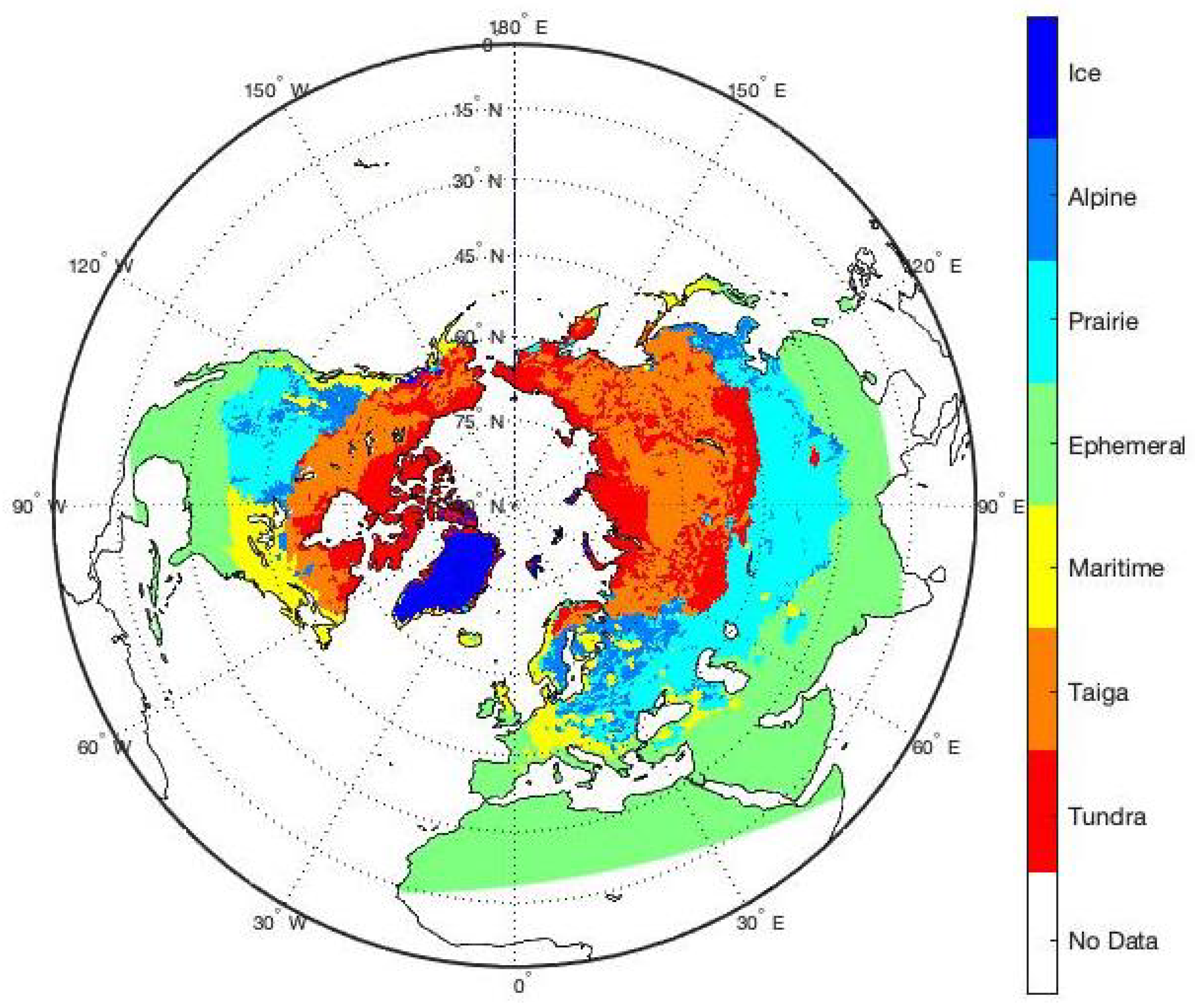
Figure 2.
Satellite viewing extent simulation of the hypothetical Ku-band SAR in Table 1 for (a) nadir points for the ascending pass during a 1-day integration period; and (b) viewing extent for the ascending pass during a 1-day integration period.
Figure 2.
Satellite viewing extent simulation of the hypothetical Ku-band SAR in Table 1 for (a) nadir points for the ascending pass during a 1-day integration period; and (b) viewing extent for the ascending pass during a 1-day integration period.
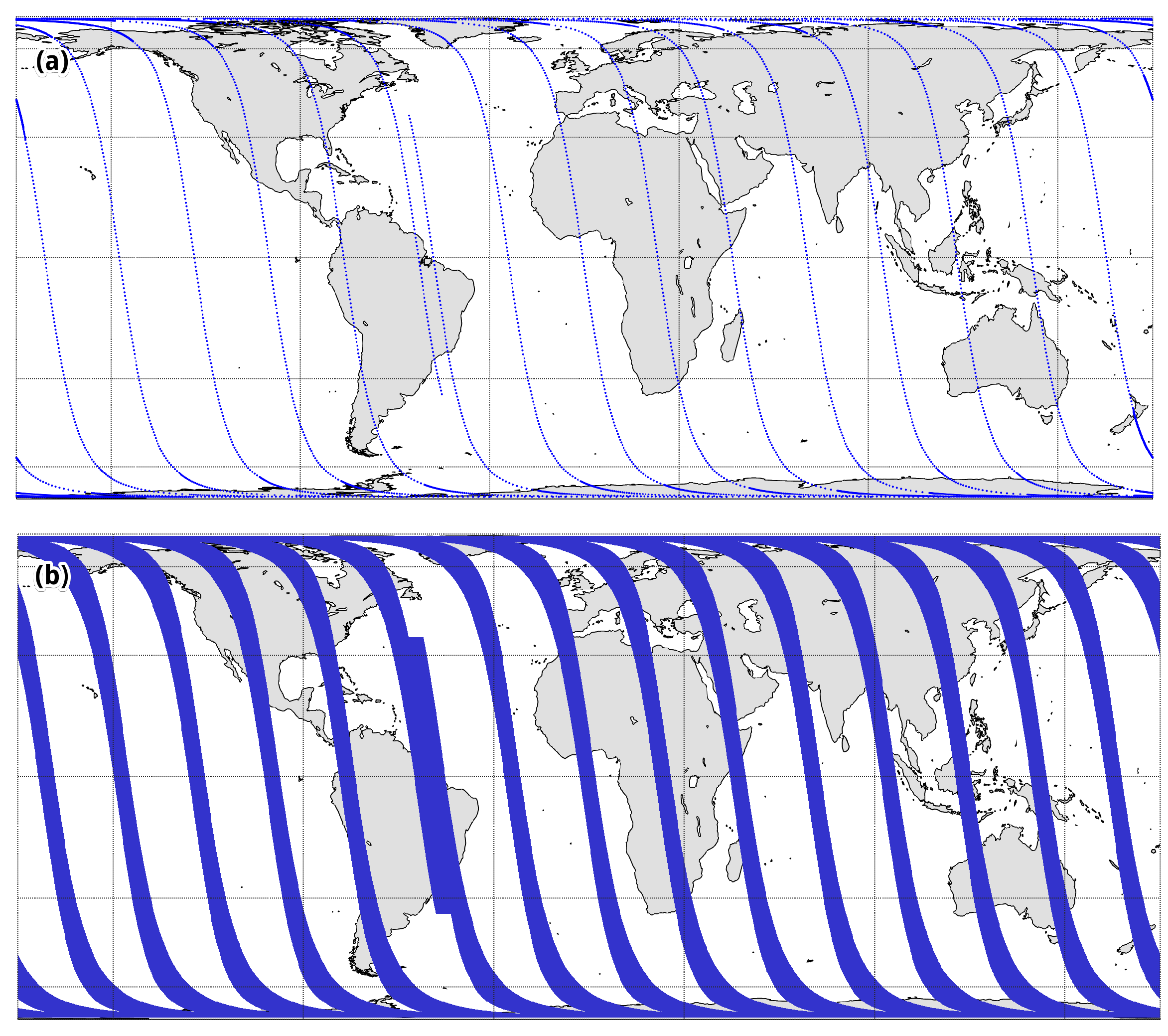
Figure 3.
Example of daily viewing extent of sensors listed in Table 1.
Figure 3.
Example of daily viewing extent of sensors listed in Table 1.

Figure 4.
Viewing example for a single day using a C-band SAR (No.3 in Table 1) overlying the snow-covered area via IMS; blue is sensor coverage; green is snow-covered terrian according to IMS.
Figure 4.
Viewing example for a single day using a C-band SAR (No.3 in Table 1) overlying the snow-covered area via IMS; blue is sensor coverage; green is snow-covered terrian according to IMS.
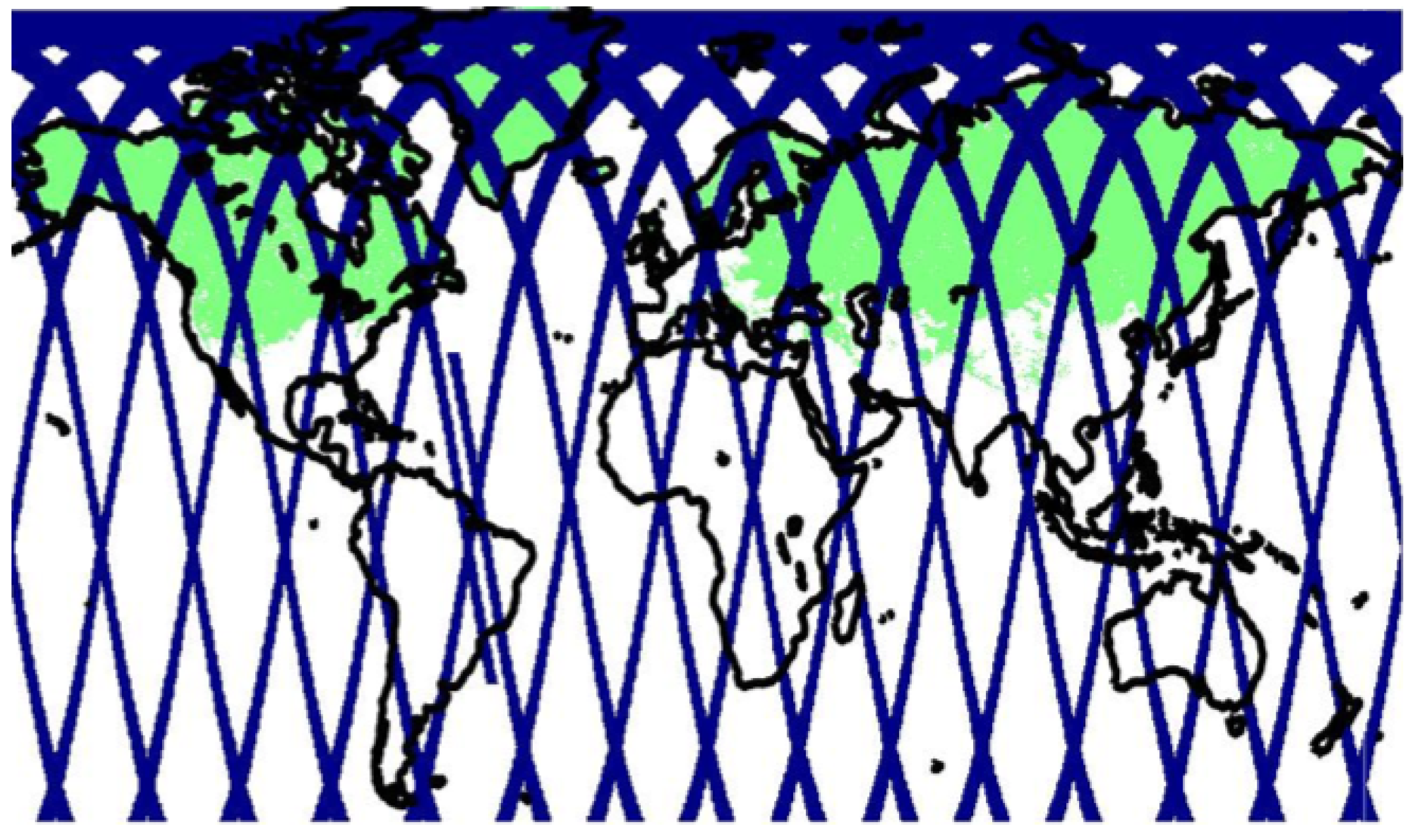
Figure 5.
Seasonal variation in viewed terrestrial snow area for different types of existing and hypothetical sensors. Subplot (a) shows coverage based on a 1-day integration period; (b) shows a 3-day integration period; (c) shows a 30-day integration period.
Figure 5.
Seasonal variation in viewed terrestrial snow area for different types of existing and hypothetical sensors. Subplot (a) shows coverage based on a 1-day integration period; (b) shows a 3-day integration period; (c) shows a 30-day integration period.
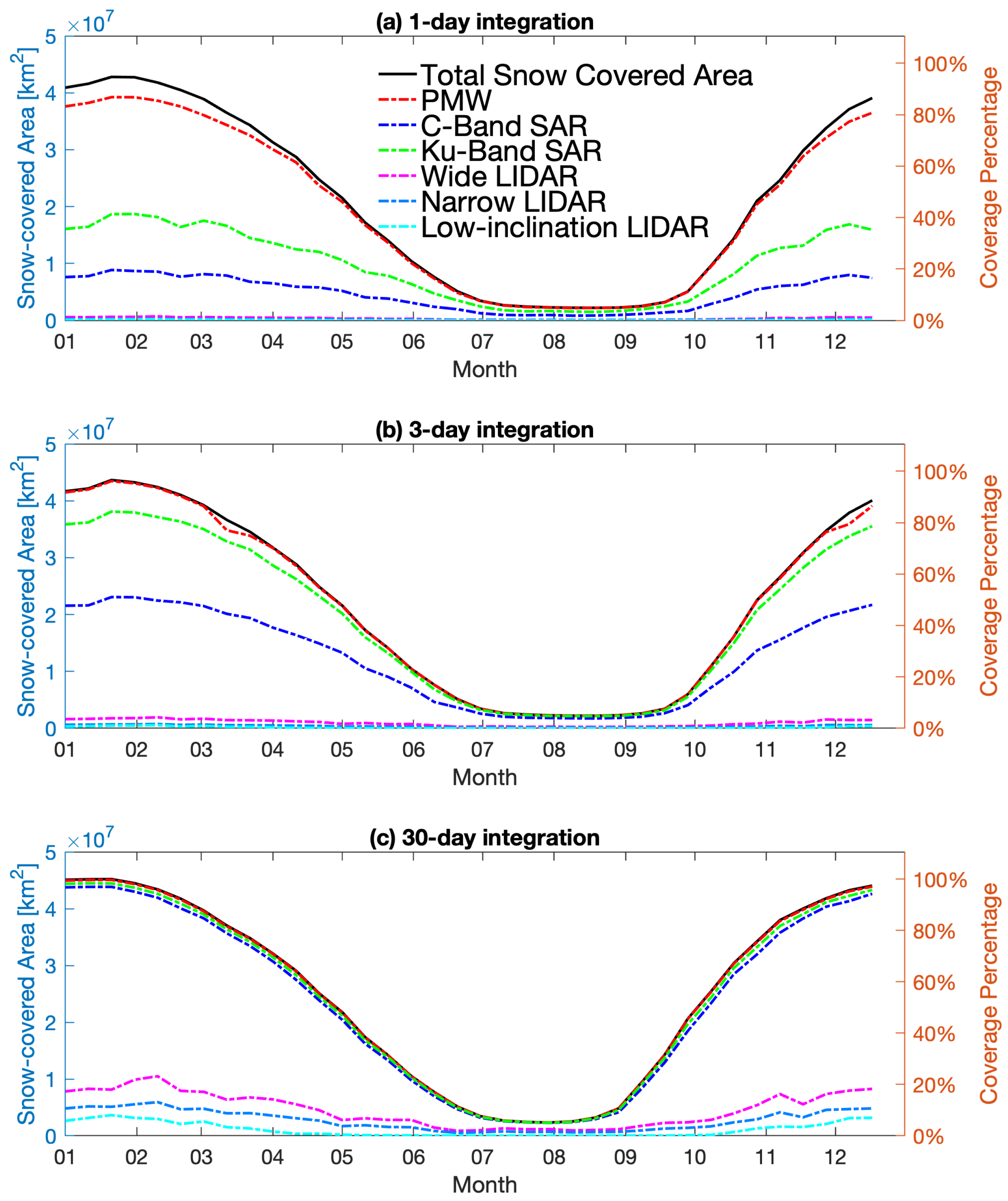
Figure 6.
Viewed snow coverage percentage as a function of orbit swath width for 1-day, 3-day, and 30-day integration periods during the month of February near peak accumulation of snow in the northern hemisphere. The dot-dashed line represents 80% viewed snow coverage.
Figure 6.
Viewed snow coverage percentage as a function of orbit swath width for 1-day, 3-day, and 30-day integration periods during the month of February near peak accumulation of snow in the northern hemisphere. The dot-dashed line represents 80% viewed snow coverage.


Table 1.
Orbital configurations of the tested sensors. The sensor prototype and its status (existing or hypothetical) is marked in “Prototype” column.
Table 1.
Orbital configurations of the tested sensors. The sensor prototype and its status (existing or hypothetical) is marked in “Prototype” column.
| ID | Sensor Type | Orbit Altitude [km] | Inclination Angle [°] | Swath Width [km] | Prototype (Status) |
|---|---|---|---|---|---|
| 1 | PMW Radiometer | 510 | 97 | 1450 | AMSR2 (Existing) |
| 2 | Ku-band SAR | 705 | 98 | 500 | TSMM (Hypothetical) |
| 3 | C-band SAR | 705 | 98 | 250 | Sentinel-1 A/B (Existing) |
| 4 | Wide LiDAR | 481 | 92 | 20 | ICESat-2 (Hypothetical) |
| 5 | Narrow LiDAR | 481 | 92 | 6 | ICESat-2 (Existing) |
| 6 | Low-inclination LiDAR | 415 | 51.6 | 6.5 | GEDI (Existing) |
PMW = passive microwave; SAR = synthetic aperture RADAR; LiDAR = light detection and ranging; AMSR2 = Advanced Microwave Scanning Radiometer 2 (AMSR2); TSMM = Terrestrial Snow Mass Mission; ICESat-2 = Ice, Cloud and land Elevation Satellite-2; GEDI = Global Ecosystem Dynamics Investigation
Table 2.
Sensor makeup of hypothetical snow constellation configurations.
| Constellation ID | Sensor Marks | Sensor Mixture |
|---|---|---|
| C1 | ✠★★\ | PMW & two C-band SARs & narrow LiDAR |
| C2 | ✠✮\ | PMW & Ku-band SAR & narrow LiDAR |
| C3 | ✠✮  | PMW & Ku-band SAR & wide LiDAR |
| C4 | ✠★★✮\ | PMW & two C-band SARs & Ku-band SAR & |
| narrow LiDAR & wide LiDAR |
✠ = PMW sensor; ★ = C-band SAR; ✮ = Ku-band SAR; \ = narrow LiDAR; ![Remotesensing 14 00633 i001]() = wide LiDAR.
= wide LiDAR.
= wide LiDAR.
Table 3.
Assumed weight of sensor efficacy, , for snow mass estimation in each snow class, j. Individual weights are subjective but serve as an effective skill estimate for each sensor relative to one another.
Table 3.
Assumed weight of sensor efficacy, , for snow mass estimation in each snow class, j. Individual weights are subjective but serve as an effective skill estimate for each sensor relative to one another.
| Tundra | Taiga | Maritime | Ephemeral | Prairie | Alpine | |
|---|---|---|---|---|---|---|
| Radiometer | 1 | 0 | 0 | 1 | 1 | 0 |
| SAR | 1 | 0 | 1 | 1 | 1 | 1 |
| LiDAR (cloud-free) | 1 | 1 | 1 | 1 | 1 | 1 |
| LiDAR (cloud-covered) | 0 | 0 | 0 | 0 | 0 | 0 |
0 = contains no skill; 1 = contains skill.
Table 4.
Effective coverage of sensors (in units of percent) for different snow classes with integration periods of 1 day, 3 days, and 30 days. Values greater than 80% are in bold font.
Table 4.
Effective coverage of sensors (in units of percent) for different snow classes with integration periods of 1 day, 3 days, and 30 days. Values greater than 80% are in bold font.
| Snow Class | |||||||
|---|---|---|---|---|---|---|---|
| Sensor ID | Tundra | Taiga | Maritime | Ephemeral | Prairie | Alpine | |
| 1-day | PMW | 98.8 | 0.00 | 0.00 | 67.1 | 77.0 | 0.00 |
| Ku-band SAR | 55.2 | 0.00 | 34.5 | 22.1 | 25.2 | 33.5 | |
| C-band SAR | 29.3 | 0.00 | 17.5 | 10.2 | 12.5 | 17.9 | |
| Wide LiDAR | 1.88 | 1.83 | 0.795 | 0.802 | 0.768 | 1.61 | |
| Narrow LiDAR | 0.686 | 0.374 | 0.316 | 0.344 | 0.346 | 0.447 | |
| Low-inclination LiDAR | 0.0901 | 0.105 | 0.211 | 0.522 | 0.158 | 0.163 | |
| 3-day | PMW | 100 | 0.00 | 0.00 | 93.7 | 95.8 | 0.00 |
| Ku-band SAR | 93.8 | 0.00 | 80.5 | 58.5 | 63.7 | 75.8 | |
| C-band SAR | 68.6 | 0.00 | 47.4 | 30.6 | 35.7 | 46.1 | |
| Wide LiDAR | 5.20 | 3.71 | 2.08 | 2.44 | 2.07 | 2.73 | |
| Narrow LiDAR | 1.92 | 1.14 | 0.832 | 1.04 | 0.911 | 0.913 | |
| Low-inclination LiDAR | 0.269 | 0.303 | 0.597 | 1.17 | 1.23 | 0.519 | |
| 30-day | PMW | 100 | 0.00 | 0.00 | 98.2 | 97.8 | 0.00 |
| Ku-band SAR | 97.7 | 0.00 | 96.0 | 93.3 | 90.3 | 94.3 | |
| C-band SAR | 94.9 | 0.00 | 91.5 | 87.7 | 82.2 | 88.9 | |
| Wide LiDAR | 18.3 | 13.8 | 8.84 | 11.4 | 9.22 | 9.70 | |
| Narrow LiDAR | 10.6 | 7.80 | 5.18 | 7.00 | 5.32 | 5.18 | |
| Low-inclination LiDAR | 2.00 | 2.12 | 3.60 | 8.20 | 7.30 | 3.01 | |
Table 5.
Percent effective viewing coverage in taiga snow regions using PMW radiometers in conjunction with efficacies ranging from 0.1 to 0.5. The different rows represent different integration periods.
Table 5.
Percent effective viewing coverage in taiga snow regions using PMW radiometers in conjunction with efficacies ranging from 0.1 to 0.5. The different rows represent different integration periods.
| Integration Period | Efficacy | ||||
|---|---|---|---|---|---|
| 0.1 | 0.2 | 0.3 | 0.4 | 0.5 | |
| 1-day | 9.8 | 20 | 29 | 39 | 49 |
| 3-day | 9.9 | 20 | 30 | 40 | 50 |
| 30-day | 10 | 20 | 30 | 40 | 50 |
Table 6.
Domain-average repeat intervals (in units of days) for different snow sensors as a function of snow class and sensor efficacy (see Table 3).
Table 6.
Domain-average repeat intervals (in units of days) for different snow sensors as a function of snow class and sensor efficacy (see Table 3).
| Snow Class | ||||||
|---|---|---|---|---|---|---|
| Sensor ID | Tundra | Taiga | Maritime | Ephemeral | Prairie | Alpine |
| PMW | 1.03 | - | - | 1.54 | 1.31 | - |
| Ku-band SAR | 2.12 | - | 3.40 | 4.61 | 3.92 | 3.07 |
| C-band SAR | 4.15 | - | 6.76 | 9.11 | 7.77 | 6.08 |
| Wide LiDAR | 64.1 | 61.3 | 179 | 75.1 | 93.1 | 85.0 |
| Narrow LiDAR | 172 | 159 | 450 | 172 | 221 | 210 |
| Low-inclination LiDAR | 390 | 400 | 332 | 136 | 138 | 292 |
Table 7.
Effective viewing coverage (in units of percent) of constellations for different snow classes with 1-day, 3-day, and 30-day integration periods. Values greater than 80% are in bold font.
Table 7.
Effective viewing coverage (in units of percent) of constellations for different snow classes with 1-day, 3-day, and 30-day integration periods. Values greater than 80% are in bold font.
| Snow Class | |||||||
|---|---|---|---|---|---|---|---|
| Constellation ID | Tundra | Taiga | Maritime | Ephemeral | Prairie | Alpine | |
| 1-day | (a) | 97.8 | 0.710 | 34.5 | 77.1 | 90.9 | 25.6 |
| (b) | 98.8 | 0.710 | 29.0 | 72.7 | 91.4 | 32.1 | |
| (c) | 98.7 | 1.83 | 29.6 | 72.9 | 91.4 | 33.8 | |
| (d) | 98.7 | 2.54 | 47.6 | 78.3 | 93.4 | 42.0 | |
| 3-day | (a) | 100 | 2.00 | 68.9 | 98.0 | 99.0 | 67.4 |
| (b) | 100 | 2.00 | 74.2 | 98.0 | 99.2 | 81.4 | |
| (c) | 100 | 5.19 | 74.7 | 98.1 | 99.2 | 81.8 | |
| (d) | 100 | 7.14 | 87.3 | 98.4 | 99.3 | 87.0 | |
| 30-day | (a) | 100 | 19.7 | 95.9 | 98.9 | 99.0 | 98.4 |
| (b) | 100 | 19.7 | 96.8 | 98.8 | 99.1 | 99.0 | |
| (c) | 100 | 44.5 | 96.9 | 98.9 | 99.1 | 99.0 | |
| (d) | 100 | 49.2 | 97.8 | 99.2 | 99.2 | 99.2 | |
Publisher’s Note: MDPI stays neutral with regard to jurisdictional claims in published maps and institutional affiliations. |
© 2022 by the authors. Licensee MDPI, Basel, Switzerland. This article is an open access article distributed under the terms and conditions of the Creative Commons Attribution (CC BY) license (https://creativecommons.org/licenses/by/4.0/).
Share and Cite
MDPI and ACS Style
Wang, L.; Forman, B.A.; Kim, E. Exploring the Spatiotemporal Coverage of Terrestrial Snow Mass Using a Suite of Satellite Constellation Configurations. Remote Sens. 2022, 14, 633. https://doi.org/10.3390/rs14030633
AMA Style
Wang L, Forman BA, Kim E. Exploring the Spatiotemporal Coverage of Terrestrial Snow Mass Using a Suite of Satellite Constellation Configurations. Remote Sensing. 2022; 14(3):633. https://doi.org/10.3390/rs14030633
Chicago/Turabian StyleWang, Lizhao, Barton A. Forman, and Edward Kim. 2022. "Exploring the Spatiotemporal Coverage of Terrestrial Snow Mass Using a Suite of Satellite Constellation Configurations" Remote Sensing 14, no. 3: 633. https://doi.org/10.3390/rs14030633
Note that from the first issue of 2016, this journal uses article numbers instead of page numbers. See further details here.