Post-Fire Forest Vegetation State Monitoring through Satellite Remote Sensing and In Situ Data

Abstract

Wildfires have significant environmental and socio-economic impacts, affecting ecosystems and people worldwide. Over the coming decades, it is expected that the intensity and impact of wildfires will grow depending on the variability of climate parameters. Although Bulgaria is not situated within the geographical borders of the Mediterranean region, which is one of the most vulnerable regions to the impacts of temperature extremes, the climate is strongly influenced by it. Forests are amongst the most vulnerable ecosystems affected by wildfires. They are insufficiently adapted to fire, and the monitoring of fire impacts and post-fire recovery processes is of utmost importance for suggesting actions to mitigate the risk and impact of that catastrophic event. This paper investigated the forest vegetation recovery process after a wildfire in the Ardino region, southeast Bulgaria from the period between 2016 and 2021. The study aimed to present a monitoring approach for the estimation of the post-fire vegetation state with an emphasis on fire-affected territory mapping, evaluation of vegetation damage, fire and burn severity estimation, and assessment of their influence on vegetation recovery. The study used satellite remotely sensed imagery and respective indices of greenness, moisture, and fire severity from Sentinel-2. It utilized the potential of the landscape approach in monitoring processes occurring in fire-affected forest ecosystems. Ancillary data about pre-fire vegetation state and slope inclinations were used to supplement our analysis for a better understanding of the fire regime and post-fire vegetation damages. Slope aspects were used to estimate and compare their impact on the ecosystems’ post-fire recovery capacity. Soil data were involved in the interpretation of the results.

1. Introduction

Forest disturbance cycles are associated with exacerbating responses to climate change [1]. Forest fires have been more frequent and severe in recent decades, especially in areas that have experienced climate change pressures for an extended period of time [2]. Due to climate change, high-temperature anomalies continue to occur, which leads to frequent forest fires [3]. The International Panel on Climate Change (IPCC) puts the Mediterranean and its adjacent lands as amongst the most vulnerable regions to the effects of global warming worldwide [4]. The models issued by IPCC agreed on a clear trend of the thermal regime based on a scenario from 1980–2000. An increase in average surface temperatures, ranging between 2.2 °C and 5.1 °C, for the period 2080–2100 was prognosed. For the same period, the models indicated pronounced rainfall regime changes showing that precipitation over lands might decrease by about 4% to 27%. Studies performed by the Department of Meteorology at the National Institute of Meteorology and Hydrology at the Bulgarian Academy of Sciences (NIMH-BAS) predicted an increase in the annual air temperature by more than 1.8 °C for the coming decades in Bulgaria. This fact increases the risk of forest fire frequency and intensity [5]. During the last two decades in Bulgaria, as well as in other countries of the Mediterranean region, many wildfires occurred and had a significant economic, political, social, and ecological impact [6,7,8,9].

In recent years, high resolution (HR) and very high resolution (VHR) optical remote sensing has become widespread concerning monitoring needs, and these strategies provide affordable multitemporal and multispectral pictures of the considered phenomena at different scales. Satellite sensors allow measurement of the impact of fires by comparing pre- and post-fire information. Applications of remote sensing technology related to fire ecology, including fire risk mapping, fuel mapping, burn severity assessment, and post-fire vegetation recovery, are widely discussed and accepted [10,11,12,13,14,15]. These technologies provide a low-cost, multi-temporal means for conducting local, regional, and global-scale fire ecology research. Moreover, the development of new technologies and techniques resulted in their rapid evolution, thus increasing the accuracy and efficiency of earth observation studies and applications [16,17]. Space and airborne sensors have been used to map burned areas, quantify the impact of fire on vegetation over large areas, and characterize post-fire ecological effects [18,19,20]. Emphasis has been given to the roles of multispectral sensors, lidar, and emerging Unmanned Aerial System (UAS) technologies [14]. Depending on the purpose of post-fire vegetation recovery observation and study, the assessment is performed based on groups of methods, such as image classification, vegetation indices (VIs), spectral mixture analysis (SMA) [21,22], etc. Remote sensing imagery offers an opportunity for obtaining land use and land cover information through image interpretation and classification. Spectral responses are used in image classification to identify the healthy vegetation in individual pixels [14]. Spectra-based classification approaches are conceptually simple and easy to implement [23]. The type or condition of surface features and their dynamics can be assessed by multi-temporal imaging. This type of analysis is fundamental in remote sensing and is typically called change detection [24]. VIs are the most commonly used method for assessments of vegetation state, including vegetation recovery after natural or anthropogenic disturbances [17,25,26].

Post-fire-related conditions are important for forest vegetation recovery. In this context, mapping of the burned area, representing the burn severity, is a standard technique for monitoring the post-fire effects and forest recovery patterns [17,27,28,29]. It was found that the differenced Normalized Burn Ratio (dNBR) and its relative form (relative differenced Normalized Burn Ratio (RdNBR)) derived from Landsat data correlate with field measurements of burn severity [30]. NBR is also used for monitoring post-fire regeneration over burned areas in ecosystems. Results showed that as vegetation regenerates, the differences between the burns and the reference area for the vegetation index decrease with time [31]. Detailed studies showed that the NIR-based vegetation indices are most appropriate for accurately assessing vegetation recovery [32]. The NDVI is found to be the most used for post-fire recovery studies, as it could be calculated alone without additional field data collection [26,33,34]. However, due to reaching saturation levels before the point where an ecosystem fully recovers its maximum biomass after disturbance, the forest recovery rate could be overestimated when using NDVI [35,36]. For estimations of variations in chlorophyll content and its changes in vegetation after a fire event, the Modified Chlorophyll Absorption Ratio Index (MCARI2) is used [37]. A quantitative analysis of forest degradation resulting from forest fires is performed by introducing the Normalized Differential Greenness Index (NDGI) [38]. The remotely sensed Moisture Stress Index (MSI) is used for canopy stress analysis and is suitable for monitoring coniferous forests and assessing specific damages that cannot be detected using NIR/R vegetation indices [39]. Spectral indices are also used to estimate other ecological parameters related to vegetation recovery. Such parameters are the Leaf Area Index (LAI) [40], the Forest Recovery Index (FRI), and Fractional Vegetation Cover (FVC) [29].

However, differences in fire severity provoke contrasting plant cover and floristic composition when ecosystems recover after forest fires. A multitude of factors such as climate, initial plant mortality, soil characteristics, the topography of the region, and vegetation composition determine the rate of recovery [41,42]. Moreover, vegetation response to fire and post-fire recovery processes differ in the various biogeographical regions and depend on vegetation type and pre-fire vegetation state [43]. For that reason, post-fire vegetation recovery is a complicated process that cannot be assessed by the application of a single, unified spectral index. Despite the advantages of spectral indices for monitoring post-fire vegetation recovery, there is still no single spectral index suitable for assessment of post-fire disturbances or vegetation recovery processes in every ecosystem, scale, and time-lag condition [44]. Even the NBR and its derivative indices developed specifically for fire-affected areas show varying accuracy under different conditions. The NBR and dNBR are considered advantageous for immediate post-fire monitoring, but their accuracy decreases with increasing temporal distance from the fire event and with the progress of vegetation recovery [45]. On the other hand, the Disturbance Index (DI) [46] is effective in monitoring forest disturbances of different origins and their temporal dynamics [47,48]. Due to the involvement of a larger range of spectral information, the DI is considered more accurate in assessing the recovery of undergrowth in forest ecosystems compared to standard monitoring methods using VIs [19,47]. The DI is based on a linear orthogonal transformation of multispectral satellite images [49,50], which increases its ability to differentiate the three main components: soil, vegetation, and moisture [51]. As a result of a fire, these three components are altered to the greatest extent. The DI more precisely separates the unvegetated spectral signatures closely linked to the stand-replacing disturbance from all other forest signatures [46]. This feature makes the DI particularly suitable for monitoring the dynamics of post-fire vegetation recovery.

This paper dissects the forest vegetation recovery stages during a period of six years after a wildfire in the Ardino region in Bulgaria. The study aims to present the potential for exploiting remotely sensed imagery and respective indices of greenness, moisture, and fire severity from Sentinel-2 to support post-fire observation and forest management with an emphasis on fire-affected territory mapping, vegetation damage assessment, fire and burn severity assessment, and their influence on the ability of vegetation to recover. The study used two groups of spectral indices for monitoring the area affected by the wildfire. The first group encompassed VIs using individual spectral bands for their calculation, and the second group included indices utilizing a larger range of spectral information through the orthogonalization of multispectral data. The Normalized Difference Vegetation Index (NDVI), the Modified Chlorophyll Absorption Ratio Index (MCARI2), and the Moisture Stress Index (MSI) are the indices that belong to the first group, and the Normalized Differential Greenness Index (NDGI), the Normalized Differential Wetness Index (NDWNI), and the Disturbance Index (DI) are the indices from the second group. The study took into account the landscape characteristics of the area influencing the processes occurring in fire-affected forest ecosystems and their post-fire recovery dynamics. Ancillary data about pre-fire vegetation state and slope inclinations were used to supplement our analysis for a better understanding of the fire regime and post-fire vegetation damages. Slope aspects were used to estimate and compare their impact on the ecosystems’ resilience, vulnerability, and post-fire recovery capacity. Soil data were involved in the interpretation of the results.

2. Materials and Methods

2.1. Study Area

The study area was situated in the southeastern part of the Rhodope Mountains, near Ardino town. The X and Y coordinates of the centroid were calculated to be 25°6′7″E and 41°34′30″N. A significant fire took place on 29 July 2016 in the study area (Figure 1). 2016 was the year with the highest wind speed during the summer months of the study period (2016–2021). The average wind speed in the summer of 2016 ranged between 4.7 m/s (in September) and 6.1 m/s (in August), and the average maximum wind speed was between 7.4 m/s (in September) and 8.1 m/s (in July) [52]. Generally, based on hourly weather simulations over the past 30 years in the study area, the maximum wind speed was observed in March (reaching up to 20 m/s average value) and the minimum windspeed was in September (starting from 3 m/s average value). Days with wind speeds above 12 m/s predominated between February and September, and days with wind speeds above 5 m/s predominated between October and January. The wind direction was mainly from the north and northwest [53].

The area affected by the forest fire was 100 ha. The main tree species were Scots pine (Pinus sylvestris L.) and Black pine (Pinus nigra Arn.). The endemic vegetation in the region refers to the Thracian province of the European deciduous forest area with the main tree species being Quercus frainetto and Q.cerris. On karst terrains, Q. frainetto, Q. cerris, and Q.pubescens, mixed with Carpinus orientalis, Fraxinus ornus, Syringa vulgaris, Cotinus coggygria, and Ostrya carpinifolia can be found [54]. However, because of erosion processes in the 1950s and the expansion of bare lands, massive afforestation with coniferous species has been performed.

Lithogenic diversity was represented by pre-Paleozoic and Paleozoic metamorphic rocks and phyllitoids covered by a Paleogene volcanogenic–sedimentary complex [54]. The terrain was hilly with steep slopes (>15°). It influenced the fire regime and is also considered a condition for the development of water erosion. Approximately 70% of the area contained slopes above 15°. The mean value of the slopes was 16° and the maximum was 27°. The slopes predominantly had east, southeast, and south exposures and define warm and dry conditions for vegetation development. The soils were shallow Lithosols mixed with Rendzinas [54].

The study area has a Continental Mediterranean climate with hot summers and mild winters. The minimum amount of precipitation is in summer, and the maximum amount is in winter. Over the last 40 years, a clear trend towards an increase in both average air temperature and precipitation sum has been observed. The average air temperature change showed a linear trend with an increase of 2.2 °C, starting from 10.2 °C in 1979 and reaching up to 12.4 °C in 2021. Summer is getting hotter, with temperatures in July and August consistently higher for the past 16 years. On the other hand, the precipitation sums in the summer months decreased, especially in August, showing a persistent negative tendency during the last 14 years. The winter is getting warmer too. February has been distinguished by sustained higher average air temperatures since 2012. The precipitation sum has also increased during the winters. Overall, there has been an increase (by 126 mm) in precipitation sum over the past 40 years. This increase is primarily due to increased winter precipitations [53]. The indicated climate changes have led to the transition of the studied area from a Warm-summer Mediterranean climate (Csb), according to the Köppen climate classification, to a Hot-summer Mediterranean climate (Csa). In addition, the slopes in the area, which predominantly had east, southeast, and south exposures, determined warm and dry conditions for the development of vegetation. The observed trends significantly increase the risk of fires in the area, loss of biological diversity, and degradation of ecosystems.

2.2. Characteristics of Climatic Anomalies Observed during the Period of 2016–2021

Figure 2 shows the mean air temperature and precipitation sum anomalies for the period of 2016–2021 on an annual basis and for the summer months (July, August, and September). As a reference, the period between 1981 and 2010 was used.

In terms of mean air temperature, 2019 was the year with the highest positive anomaly (+1.4 °C). Amongst the summer months, August was with positive anomalies only. The highest anomalous value (+1.6 °C) was recorded in 2017. The highest anomalous value for the summers between 2016 and 2021 was recorded in September 2020 (+2.6 °C). Three of the years during the period of 2016–2021 were characterized by positive anomalies in all three summer months. Overall for the three summer months, 2020 was with the highest positive anomaly (+4.7°C). The lowest positive anomaly, overall for the three summer months, was recorded in 2018 (+0.3°C). The mean air temperature in July 2018 was 1 °C lower in comparison with the reference period (Figure 2a) [52].

Higher sums of annual precipitation were observed during the period of 2016–2021. The wettest year was 2021, which had a 36% higher precipitation sum in comparison with the reference period. There was no definite trend in the distribution of precipitation during the summer months. All three summer months of 2016 and 2020 had lower precipitation. In 2020, the total precipitation for the summer was 106% lower in comparison with the reference period. In September 2020 only, the precipitation sum was lower by 83%. The wettest summer was in 2019. In that summer, the total amount of precipitations was 366% higher in comparison with the reference period (Figure 2b) [52].

2.3. Data

2.3.1. In Situ Data

In situ data included climatic data, soil data, and field observations.

The climatic data were based on measurements at the Kardzhali meteorological station (331 m.a.s.l) situated 21 km from Ardino [53] and on hourly weather simulations with 30 km spatial resolution over the past 30 years [52]. The in situ climatic data included mean air temperature and precipitation sum for a period between 1979 and 2021 as well as data about the mean air temperature and precipitation sum anomalies for the period of 2016–2021 on an annual basis and for the summer months (July, August, and September) [53]. In addition, ERA5 model data, which combined satellite and in situ historical observation, were used to outline how climate change has already affected the Ardino region in the last 40 years [52].

The soil data included soil types [54], soil chemical composition, and organic matter content, which were measured in a pine-dominated mixed woodland (790 m.a.s.l) situated near Ardino in 2015 [55]. Soil field data is part of LUCAS 2015 Topsoil datasets, which is freely available through the European Soil Data Centre (ESDAC) of the Joint Research Centre [55]. Because the soil data refer to the pre-fire period and the soil samples were not taken from the affected area specifically, they were used only for result interpretation as auxiliary data.

Interactive three-dimensional panoramas were used as a means of field observations. They were acquired via Google Street View technology in the summer of 2021. These were used to generate high-quality photographs of eight locations affected by the fire [56].

2.3.2. Satellite Data

Satellite data acquired from Sentinel-2A and Sentinel-2B multispectral sensors of the European Space Agency Program for Earth Observation “Copernicus” [57] were used to assess post-fire vegetation recovery. The temporal resolution of every individual Sentinel-2 satellite is ten days, and their combined resolution is five days. More detailed information about the spectral and spatial resolution of the Sentinel-2 satellites can be found in

Table A1. Spectral (in microns) and spatial (in meters) resolution of Sentinel-2 sensor.

Band	Spectral Resolution	Spatial Resolution
B1	0.443	60
B2	0.49	10
B3	0.56	10
B4	0.665	10
B5	0.705	20
B6	0.74	20
B7	0.783	20
B8	0.842	10
B8a	0.865	20
B9	0.94	60
B10	1.375	60
B11	1.61	20
B12	2.19	20

[57].

The Sentinel-2 image acquired on 10 July 2016 was representative for the period before the fire event (29 July 2016), and the images acquired on 24 August 2017 and 2018, 14 August 2019, 02 September 2020, and 23 August 2021 were used for assessment of the forest vegetation state after the fire.

High-resolution forest layers (HRLs), which are freely available through the Copernicus Land Monitoring Service [58], were used in the validation process. The layers included Tree Cover Density (TCD) and Forest Type (FTY) products. The TCD product represents the level of tree cover density in a range from 0–100% for 2012, 2015, and 2018 reference years. The Forest Type product represents the dominant leaf type with a Minimum Map Unit (MMU) of 0.5 ha. Both products are pixel-based, and the minimum mapping width is 20 m. The forests’ HRLs in 2015 were verified for the territory of Bulgaria using in situ data [59]. The verification procedure was performed on three levels, including the highly recommended quantitative verification. According to the results obtained by Tepeliev et al. [59], the HRLs used in the present study are generally correctly mapped for the territory of Bulgaria. Hence, we assumed that they could be used as independent reference data in the validation procedure.

A Digital Elevation Model (DEM) with a spatial resolution of 25 m was used to obtain slopes and slopes’ aspects. The dataset is freely available through the Copernicus Land Monitoring Service [60].

2.4. Methods

The proposed approach for monitoring post-fire vegetation state and estimating its dynamics included the following basic steps. First, spectral indices for the period between 2016 and 2021 were calculated to assess forest vegetation recovery dynamics. Second, statistical regression analyses using three of the spectral indices as variables were performed. The indices involved in the linear regression analyses were DI, MCARI2, and MSI. These indices are representative of key post-fire characteristics of the affected territories. The DI was used for the assessment of disturbance of forest ecosystems, burn severity, and vegetation damage. MCARI2 is representative for vegetation regrowth, and MSI shows stress in ecosystems caused by moisture deficiency. The third step considered differences in landscapes and the conditions for forest recovery they create, which is predetermined by the impact of slope exposures and their influence on the heat–moisture ratio. The assessment of the slope exposure factor was based on a differentiated evaluation of indices dynamics and their interpretation. The final step consisted of the validation of obtained results using statistical regression analyses involving the forest HRLs as independent reference data. Interactive three-dimensional panoramas from Google Street View were also used in the validation process. The interactive panoramas were used to generate photographs in different directions in order to demonstrate the state of various ecosystems. X and Y coordinates and altitude of the point locations of the photographs were extracted. The obtained point locations were georeferenced and digitized to be used in overlay analyses with the indices’ rasters. The eight locations affected by the fire that were observed via this technology were linked to the obtained results as a means for field observation. For each location, indices values were extracted by taking into account the observed perspective and the distance of the objects from the point of capture.

Spectral Indices Selected for Assessment of Post-Fire Vegetation Recovery

The spectral indices presented in

Table 1. Spectral indices calculated in this study.

Index	Abbreviation	Formula
Normalized Difference Vegetation Index [61]	NDVI	$NDVI=\frac{\rho NIR-\rho RED}{\rho NIR+\rho RED}$ (1)
Modified Chlorophyll Adsorption Ratio Index [62]	MCARI2	$MCAR{I}_2=\frac{1.5\left[2.5\left({\rho }_{800}-{\rho }_{670}\right)-1.3\left({\rho }_{800}-{\rho }_{550}\right)\right]}{\sqrt{{\left(2{\rho }_{800}+1\right)}^2-\left(6{\rho }_{800}-5\sqrt{{\rho }_{670}}\right)}-0.5}\hspace{1em}\left(2\right)$
Moisture Stress Index [63]	MSI	$MSI=\frac{SWIR1}{NIR}$ (3)
Normalized Differential Wetness Index [38,64,65]	NDWNI	$NDWNI=\frac{W_n\left(t_2\right)-W_n\left(t_1\right)}{\left|W_n\left(t_2\right)\right|+\left|W_n\left(t_1\right)\right|},$ (4) $W_n\left(t\right)=\frac{W\left(t\right)-E\left\{W\left(t\right)\right\}}{St.Dev.\left[W\left(t\right)\right]},$ (5)
Normalized Differential Greenness Index [38]	NDGI	$NDGI=\frac{G{R}_n\left(t_2\right)-G{R}_n\left(t_1\right)}{\left|G{R}_n\left(t_2\right)\right|+\left|G{R}_n\left(t_1\right)\right|},$ (6) $G{R}_n\left(t\right)=\frac{GR\left(t\right)-E\left\{GR\left(t\right)\right\}}{St.Dev.\left[GR\left(t\right)\right]},$ (7)
Disturbance Index [46]	DI	DI = nBR − (nGR + nW) (8)

were selected and calculated to assess the post-fire vegetation state.

The most well-known and used vegetation index for quantifying green vegetation in the near-infrared wavelength region and chlorophyll absorption in the red wavelength region is the NDVI. The NDVI strongly correlates with climate variations and their impact on plant growth. That makes this index especially suitable for estimations of climate-related vegetation changes. Moreover, changes in NDVI values correlate with the de Martonne aridity index [19].

The MCARI has been proposed to estimate variations in chlorophyll content and its concentration changes. Unlike MCARI, the newly designed MCARI2 is less sensitive to chlorophyll concentration variations but has a high linear relationship with near-infrared canopy reflectance and high linearity with the green LAI. The LAI is an important variable used to estimate the biophysical processes of different vegetation types and predict their growth and productivity [21,62]. Both the NDVI and MCARI2 range between −1 and +1. The highest values indicate dense and “healthy” vegetation, and the lowest values indicate dead plants or inanimate objects.

The remotely sensed MSI is used for canopy stress analysis, productivity prediction, and biophysical modeling. It detects plant water stress for these plants only, which are able to tolerate low leaf water content through cellular adjustments. In the current study, the MSI is especially suitable for monitoring coniferous forests and assessing specific damages that cannot be detected using NIR/R vegetation indices [39]. Considering coniferous vegetation, the differences in the MSI between damaged and undamaged stands are not necessarily related to differences in the LAI. The MSI ranges from 0 to more than 3. Higher values indicate greater moisture stress.

Additionally, a quantitative analysis of forest degradation resulting from forest fires was performed by introducing the NDGI and the NDWNI. Both indices are based on satellite image orthogonalization. In the process of orthogonalization, three differentiable classes (soil brightness, greenness, and wetness axes) related to the main components of the Earth’s surface (soil, vegetation, and water) are obtained. The NDGI uses the greenness component, which corresponds to vegetation’s spectral reflectance characteristics (SRC), and the NDWNI uses the wetness component, which corresponds to water’s SRC. These indices quantitatively estimate the slightly positive and negative values of change in the vegetation’s green mass and moisture content for a given period [38,64,65]. Both indices range from −1 to +1. The positive NDGI values indicate plant growth and improvement of the vegetation state, and the negative values indicate deterioration of the vegetation state or deforestation. The positive NDWNI values indicate an increase in moisture content in ecosystems, and the negative values indicate a decrease in moisture content.

The DI has also been used to monitor disturbances by forest fires. The index values range widely, with positive values indicating disturbances. Higher values indicate more severe disturbance. The DI is modified by weighting each input component to maximize the difference between disturbed and undisturbed forest canopy. The weights reduce the effects of background variations while emphasizing the variations caused by disturbance [48]. The model for calculating the DI includes three steps: the first step is the decomposition of each of the three major Tasseled Cap components (brightness (BR), greenness (GR), and wetness (W)); the second step is to calculate the averages and standard deviations for each of the Tasseled Cap components; and the third step is to calculate the normalized values of the components. These steps are needed to normalize the radiometric changes. In the normalization, the following equations were used [46]:

nBR = (BR − E{BR}/St.Dev (BR)

(9)

nGR = (GR − E{GR}/St.Dev (GR)

(10)

nW = (W − E{W}/St.Dev (W)

(11)

where E {BR}, E {GR}, and E {W} are the average values of the brightness, greenness, and wetness, respectively. St.Dev (BR), St.Dev (GR), and St.Dev (W) are the respective standard deviations of these Tasseled Cap components. Therefore, nBR, nGR, and nW are the normalized values of brightness, greenness, and wetness, respectively. The DI is computed according to the equation presented in Table 1.

3. Results

3.1. Forest Vegetation Recovery for the Entire Study Area

Areas with negative NDGI values predominated until 2019. The NDGI values were negative even a year before the fire event, which indicates a degraded state of forest vegetation. The territories with negative NDGI values had maximum territorial spread in the pre-fire year and a year after the fire (Figure 3,

Table A2. Territorial spread (in %) of the individual categories divided for each of the spectral indices within the study area. This table represents the values behind the output rasters from Figure 3.

NDVI
Category	2016	2017	2018	2019	2020	2021
0–0.1	0.0	0.0	0.0	0.0	0.0	0.0
0.1–0.2	0.0	4.7	0.8	0.3	0.5	0.1
0.2–0.3	0.1	20.2	6.9	3.3	6.3	2.2
0.3–0.4	1.7	21.0	18.1	10.7	18.5	9.3
0.4–0.5	6.8	18.0	24.3	19.1	26.7	20.6
0.5–0.6	28.2	18.3	26.1	25.5	28.3	28.9
0.6–0.7	48.1	13.5	18.1	27.1	17.5	29.7
0.7–0.8	14.1	3.8	5.3	12.1	2.2	8.9
0.8–0.9	1.0	0.1	0.0	1.7	0.0	0.2
0.9–1	0.0	0.3	0.3	0.3	0.0	0.0
MCARI2
Category	2016	2017	2018	2019	2020	2021
0–0.1	0.3	0.7	0.4	0.4	0.1	0.0
0.1–0.2	0.0	3.3	0.6	0.2	0.3	0.1
0.2–0.3	0.0	10.3	2.1	1.1	2.1	0.9
0.3–0.4	0.2	13.7	6.0	3.1	6.0	3.0
0.4–0.5	1.4	14.5	11.8	7.2	13.5	7.8
0.5–0.6	3.9	14.3	18.0	13.2	20.5	15.9
0.6–0.7	11.3	15.3	20.8	20.2	21.4	22.6
0.7–0.8	47.5	19.4	25.1	29.0	26.7	29.7
0.8–0.9	35.2	8.6	15.2	25.5	9.5	20.0
0.9–1	0.1	0.0	0.0	0.3	0.0	0.0
MSI
Category	2016	2017	2018	2019	2020	2021
0.3–0.5	3.3	1.7	2.0	3.4	1.8	3.8
0.5–0.7	60.5	16.3	19.0	23.3	17.3	23.9
0.7–0.9	29.7	17.0	23.5	29.3	20.6	28.7
0.9–1.1	5.1	17.3	25.2	25.7	24.0	27.9
1.1–1.3	1.2	19.3	22.7	15.9	26.0	14.2
1.3–1.5	0.1	18.8	7.4	2.4	9.6	1.5
1.5–1.7	0.0	8.3	0.3	0.0	0.8	0.0
1.7–1.9	0.0	1.2	0.0	0.0	0.0	0.0
1.9–2.1	0.0	0.1	0.0	0.0	0.0	0.0
2.1–2.3	0.0	0.0	0.0	0.0	0.0	0.0
DI
Category	2016	2017	2018	2019	2020	2021
<0	52.1	36.4	36.6	34.9	35.9	35.9
0–1	28.8	12.3	16.2	20.6	16.9	21.8
1–2	12.1	16.2	19.4	21.9	25.4	30.0
2–3	4.0	16.9	17.7	15.9	19.4	11.7
3–4	2.0	12.3	8.6	6.0	2.4	0.6
4–5	0.7	4.9	1.5	0.6	0.0	0.0
5–6	0.2	0.9	0.0	0.0	0.0	0.0
6–6.5	0.0	0.0	0.0	0.0	0.0	0.0
>6.5	0.0	0.0	0.0	0.0	0.0	0.0
NDGI
Category	2015–2016	2016–2017	2017–2018	2018–2019	2019–2020	2020–2021
−1–−0.8	7.9	49.9	5.5	2.8	6.1	1.9
−0.8–−0.6	2.0	4.9	1.3	0.8	2.0	0.7
−0.6–−0.4	4.4	5.3	2.7	1.7	3.1	1.3
−0.4–−0.2	12.7	6.3	6.6	6.7	5.7	4.1
−0.2–0	29.7	8.3	24.8	23.5	12.5	20.5
0–0.2	26.6	10.8	22.2	32.3	26.1	29.2
0.2–0.4	8.8	7.8	11.0	13.1	18.3	14.1
0.4–0.6	4.2	3.9	6.3	5.7	9.1	7.8
0.6–0.8	2.4	2.0	4.1	3.2	4.4	4.5
0.8–1	1.2	0.8	15.5	10.2	12.6	15.8
NDWNI
Category	2015–2016	2016–2017	2017–2018	2018–2019	2019–2020	2020–2021
−1–−0.8	20.4	14.8	5.8	7.8	3.9	6.3
−0.8–−0.6	5.6	6.3	2.1	2.3	1.7	2.0
−0.6–−0.4	8.4	7.2	4.8	4.4	3.8	3.2
−0.4–−0.2	13.7	8.4	12.1	10.5	12.3	7.9
−0.2–0	22.6	10.5	22.9	34.1	32.8	28.5
0–0.2	23.2	9.5	32.8	34.8	27.0	36.2
0.2–0.4	4.9	8.7	11.6	4.4	7.7	8.8
0.4–0.6	0.6	8.2	2.8	0.6	3.4	2.4
0.6–0.8	0.2	5.7	1.2	0.3	1.9	1.3
0.8–1	0.5	20.7	4.0	0.7	5.5	3.5

). The areas in the range from −1 to −0.8 were dominant between 2016 and 2017 in the year immediately following the fire (Figure 3, Table A2). With increasing temporal distance from the fire event, the maximum territorial spread shifted to the category with slightly positive values (from 0 to 0.2). The areas with positive NDGI values, or an increase in biomass, had minimal spread in the year immediately following the fire (Figure 3, Table A2). The positive NDGI values had the highest growth between 2019 and 2020 (Figure 3, Table A2).

Surprisingly, the areas with no disturbance or negative DI values prevailed during the entire studied period (Figure 3, Table A2). However, this maximum was highest in the year before the fire event. Moreover, during the same year, the highest territorial spread of the areas with great disturbance was observed. Areas from the same category (DI > 5) were also recorded in the following 2017 and 2018 years (Figure 3, Table A2). After 2019, with increasing temporal distance from the fire event, areas falling into this category were not observed. In the year before the fire event, a large portion of the areas had DI values between 0 and 2. In 2017, the areas were almost evenly distributed in the categories with DI values between 0 and 4. In the following four years, between 2018 and 2021, the maximum spread had areas with DI values between 0 and 3 (Figure 3, Table A2).

The first post-fire year was characterized by the most pronounced stress due to moisture deficiency. In the same year, the highest territorial spread of the category with MSI values above 1.5 was also observed (Figure 3, Table A2). The MSI category with values between 0.5 and 1.5 had the largest share of the area. The maximum spread had territories with MSI between 1.1 and 1.3. In the pre-fire year, 60.5% were in the category with MSI between 0.5 and 0.7. Between 2018 and 2021, the area was concentrated in the MSI categories between 0.5 and 1.3. The maximum spread was between 0.7 and 1.3 (Figure 3, Table A2).

Regarding the NDWNI, the maximum area was mainly in the category between −0.2 and 0.2, indicating weak dynamics in the moisture content. An exception was the one-year period immediately after the fire when a significant increase in moisture content was observed (Figure 3, Table A2). In the years before the fire and between 2018 and 2021, a significantly smaller share of the area had positive NDWNI dynamics (Figure 3, Table A2).

During the year before the fire, 94% of the area had MCARI2 values above 0.6. Moreover, almost half of the area had MCARI2 values between 0.7 and 0.8. This category (0.7–0.8) also had a maximum territorial spread in the post-fire years, but the area falling into this category was significantly less (Figure 3, Table A2). In the post-fire year of 2017, the area was more evenly distributed between the individual categories. In the following years, the area was concentrated mainly in the MCARI2 category with values between 0.4 and 0.9. The share of the areas in this category gradually increased, reaching 96% in 2021 (Figure 3, Table A2).

Greater dynamics were observed in the maximum territorial spread between the individual NDVI categories. In the pre-fire year, the highest proportion of territories had NDVI values between 0.6 and 0.7, whereas in the year following the fire event, maximum spread had territories with NDVI between 0.3 and 0.4. The maximum territorial spread shifted to the categories with higher NDVI values in the years between 2018 and 2021 (Figure 3, Table A2).

3.2. Forest Vegetation Recovery in the Individual Slope Aspects

The differential analysis of the dynamics of indices values on the individual slope exposures showed that in the first three years after the fire event (2017–2019), the southwest-facing slopes had faster vegetation recovery and less moisture stress. These slopes had the highest values of the NDVI and MCARI2 and the lowest values of the MSI (

Table 2. Mean values of the spectral indices for the different slope aspects in the studied years.

Aspect	2016	2017	2018	2019	2020	2021
NDVI
E	0.63	0.37	0.47	0.54	0.54	0.59
NE	0.64	0.37	0.47	0.52	0.59	0.63
S	0.61	0.36	0.44	0.51	0.46	0.53
SE	0.61	0.40	0.46	0.53	0.45	0.52
SW	0.63	0.41	0.50	0.56	0.50	0.56
MCARI2
E	0.77	0.46	0.61	0.67	0.68	0.73
NE	0.78	0.45	0.62	0.64	0.75	0.77
S	0.76	0.46	0.57	0.64	0.58	0.65
SE	0.74	0.50	0.59	0.65	0.57	0.63
SW	0.77	0.52	0.64	0.69	0.64	0.69
MSI
E	0.64	1.20	0.99	0.93	0.85	0.75
NE	0.61	1.21	0.92	0.92	0.70	0.65
S	0.69	1.22	1.07	0.96	1.06	0.93
SE	0.72	1.15	1.02	0.93	1.07	0.93
SW	0.62	1.10	0.92	0.85	0.94	0.83
DI
E	−0.48	1.94	0.98	1.30	−0.05	−0.05
NE	−0.74	1.66	0.46	1.19	−0.18	−0.15
S	−0.09	1.85	1.63	1.39	0.11	0.09
SE	0.58	1.53	0.14	1.27	0.12	0.10
SW	−0.80	0.86	0.36	0.48	0.00	0.01
	2015–2016	2016–2017	2017–2018	2018–2019	2019–2020	2020–2021
NDWNI
E	−0.46	−0.29	0.09	−0.16	0.07	−0.05
NE	−0.70	−0.27	0.27	−0.39	0.18	−0.12
S	−0.23	−0.25	−0.10	−0.02	−0.10	0.00
SE	−0.18	0.02	−0.09	−0.03	−0.03	−0.01
SW	−0.37	−0.31	0.04	−0.17	−0.06	−0.11
NDGI
E	−0.05	−0.81	0.38	0.10	0.26	0.18
NE	−0.16	−0.76	0.38	−0.16	0.34	0.01
S	−0.02	−0.77	0.16	0.26	0.10	0.30
SE	0.00	−0.57	0.13	0.21	0.09	0.29
SW	−0.13	−0.65	0.29	0.14	0.19	0.17

). The MCARI2 had a better ability to differentiate vegetation recovery through the individual slopes. On east- and southeast-facing slopes, the NDVI showed equal totals over the three years, while the MCARI2 distinguished them. The difference in MCARI2 values between the individual slope aspects was higher than those of the NDVI and was clearer (Table 2). Regarding moisture stress in the first three years after the fire event, the MSI total values gradually increased in the following sequence: northeast-facing, southeast-facing, east-facing, and south-facing slopes (Table 2). In the last two post-fire years, the northeast-facing slopes had the highest total values of NDVI and MCARI2 and the lowest moisture stress. On northeast-facing slopes, the highest totals of NDVI and MCARI2 and the lowest totals of MSI for the entire period were recorded (Table 2).

In the pre-fire year, only the vegetation on southeast-facing slopes had positive DI values (Table 2). Moreover, territories most affected by the fire were situated on slopes with such exposure in the northern part of the area. The entire forest vegetation was destroyed in those territories (Figure 1). The fire most likely started there (Figure 3). The mean DI values were positive for all slopes in the following three post-fire years. The total DI values for the individual slope exposers for 2017, 2018, and 2019 decreased in the following sequence: south-facing, east-facing, northeast-facing, southeast-facing, and southwest-facing slopes (Table 2). Despite the higher DI values recorded for the east and northeast-facing slopes in the first three post-fire years, only these slopes had negative values in the last two years of observation (Table 2). On slopes with a southern component, the DI remained positive. In contrast to the trend observed in the NDVI, MCARI2, and MSI for the entire period, the lowest DI values and the optimal vegetation state were not recorded for the northeastern but for the southwestern slopes. However, as recorded by the listed indices, the vegetation had the worst condition on south-facing slopes (Table 2).

The other two indices based on TCT (NDWNI and NDGI) can measure small changes in moisture content and green mass. A slight positive increase in moisture content in the first post-fire year was recorded only for the southeast-facing slopes. In 2018 and 2019, the northeast-facing slopes had the highest positive NDWNI dynamics. The eastern slopes also showed positive dynamics in the moisture content in these years (Table 2).

The NDGI, or green mass, showed positive dynamics after the second post-fire year (2017–2018). In the period between 2017 and 2018, the vegetation on east- and northeast-facing slopes had the highest increase in NDGI values. These were the highest NDGI mean values in the entire period of observation and for all of the slope exposures (Table 2). Moreover, during the drought in 2020, the vegetation on the northeastern and eastern slopes again showed better condition compared to those on the slopes with different exposure (Table 2). The NDWNI dynamics were also positive for the northeast- and east-facing slopes in 2020. However, for the entire period of observation, the vegetation on southeast-facing slopes had the highest total increase in NDGI values (Table 2).

3.3. Linear Regression Analyses for the Apectral Indices

The statistical regression analyses were representative for the correlation and dependency between some of the key post-fire characteristics of the affected territories in the vegetation recovery process.

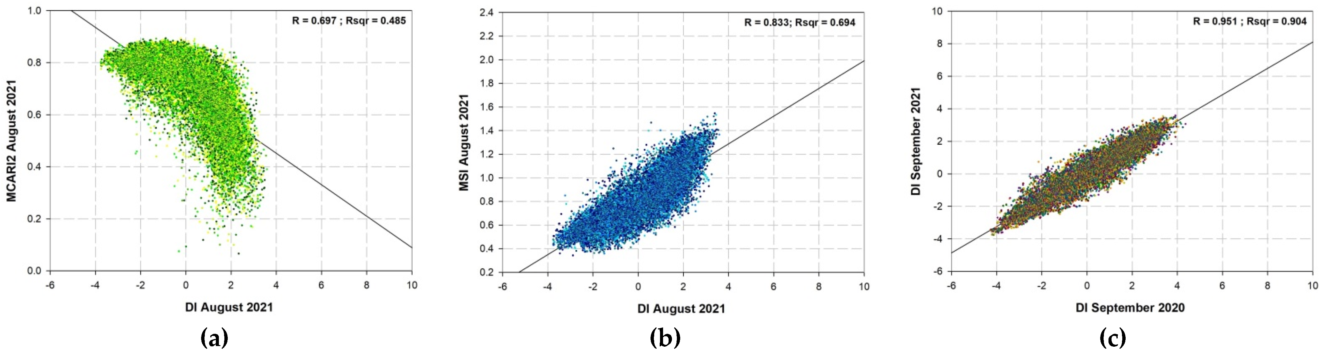
The correlation between the areas affected by disturbance increased with the development of ecosystem restoration processes and improving vegetation condition. The weaker correlation between 2017 and 2018 indicated a higher difference in the state of the forest vegetation in the first and second post-fire years (Figure 4c). This trend confirmed the rapid development of the post-fire succession process between the first and second years after the wildfire. The correlation was also lower between 2019 and 2020 when the severe drought in the summer of 2020 influenced the vegetation state and increased the intra-territorial differences. The increase in correlation for the periods between 2018 and 2019 and between 2020 and 2021, in turn, showed greater similarity in the state of the vegetation. In the second post-fire year (the period between 2018 and 2019), the higher correlation indicated delaying of the ecosystem restoration process, and in the 2020–2021 period, it indicated restoring balance in the ecosystems disturbed by the severe drought. The character of the territorial spread of vegetation throughout the individual categories divided by the DI values confirmed these observations (Figure 3, Table A2). In the first post-fire year, which was distinguished by weaker correlation, the vegetation was divided between eight categories. In 2021, as vegetation recovery progressed and the highest correlation was recorded, the number of these categories decreased to five. In 2021, 67.4% of the area was concentrated in two categories. 30% of this share consisted of the territories with DI between 1 and 2. That was the greatest share of the area falling into this category of disturbance for the entire period of observation. The area in this category gradually increased between 2016 and 2021, starting at 16.4% in 2016 and reaching up to 30% in 2021 (Figure 3, Table A2).

The correlation between MSI and DI values, in turn, showed a decreasing trend with the progression of the ecosystem restoration process (Figure 4b). In 2017 (the first post-fire year), the correlation between the disturbed ecosystems and moisture stress was highest for the entire period of observation. That indicated that for most of the forest ecosystems, higher MSI values were connected with higher DI values. In other words, the lack of moisture was connected with a higher degree of disturbance of the ecosystems (Figure 4b). The progression of ecosystem restoration processes decreased this dependency.

The correlation and the dependency between MCARI2 and DI (i.e., between leaf area and intensification of photosynthesis and the degree of disturbance of the ecosystem) showed a decreasing trend with the progression of ecosystem restoration processes for the first three post-fire years. Figure 4a shows that the areas characterized by high MCARI2 values were distinguished by lack of disturbance of the ecosystem and vice versa; areas with lower MCARI2 values (e.g., 0.2) (i.e., areas with underdeveloped vegetation and small leaf area) were distinguished by a higher degree of disturbance of the ecosystems. The progression of ecosystem restoration processes led to an increase in leaf mass and intensification of photosynthesis. The lowest MCARI2 values reached 0.4 in 2019. In these areas, the DI had decreased to below 4. The decline in the dependency between the vegetation state and the degree of disturbance of ecosystems confirmed the progression of ecosystem restoration processes. The decreasing trend in the correlation was interrupted by drought stress in 2020. In 2021, the correlations between both indices started to decline again. However, the forest recovery trend still could be observed. Starting from 2020, vegetation with DI values above 4 was not observed (Figure 4a).

3.4. Validation through HRLs

Statistical regression analyses involving the forest HRLs acquired in 2012, 2015, and 2018 as independent reference data were performed to validate the obtained results.

Generally, between 2012 and 2018, an increase in tree cover density of both broad-leaved forests and coniferous forests was observed. The largest share of the area had forests with tree cover density between 40% and 80% (

Table 3. Tree-cover density (TCD) classes (%) and area of their distribution (%) within broad-leaved and coniferous forests in 2012, 2015, and 2018.

TCD (%)	Broad-Leaved Forests			Coniferous Forests
	2012 (%)	2015 (%)	2018 (%)	2012 (%)	2015 (%)	2018 (%)
0–20	6.66	0.8	0.72	0.63	non	non
20–40	14.53	9.41	25.51	3.83	0.75	9.39
40–60	37.61	72.47	39.02	19.15	43.85	54.26
60–80	38.97	15.92	28.47	73.96	55.35	34.96
>80	2.22	1.4	6.29	2.43	0.06	1.39
Mean	43.86	52.21	56.19	47.37	55.67	60.28

). In the post-fire year of 2018, the non-forested areas, as expected, had the highest disturbance (

Table 4. Mean values of the spectral indices in broad-leaved forests, coniferous forests, and in non-forested areas in 2018.

Index	Broad-Leaved Forests	Coniferous Forests	Non-Forested Areas
DI	−7.57	−18.54	15.97
MCARI2	0.79	0.76	0.57
MSI	0.71	0.68	1.06
NDGI	0.08	−0.08	0.23
NDVI	0.65	0.59	0.44
NDWNI	−0.05	0.12	−0.06

). They had positive DI values. The DI for the forested areas in the same year was negative. The non-forested area recorded the highest moisture stress (MSI > 1) (Table 4) but also the highest increase in NDGI values. That was related to the development of vegetation succession processes in the deforested territories. The vegetation indices NDVI and MCARI2 recorded their highest values in broad-leaved forests. However, coniferous forests had the highest positive dynamics in moisture content (NDWNI) (Table 4).

The DI and MSI were the indices that showed the highest correlation with forest density (

Table 5. Linear regression between forest density (independent) and spectral indices (dependent) for each of the forest types.

	Broad-Leaved Forests		Coniferous Forests		Non-Forested Areas
Index	R	Rsqr	R	Rsqr	R	Rsqr
NDVI	0.16	0.03	0.53	0.28	0.18	0.03
MCARI2	0.46	0.21	0.51	0.26	0.18	0.03
NDGI	0.03	0	0.15	0.02	0	0
DI	0.61	0.37	0.65	0.43	0.2	0.04
MSI	0.64	0.4	0.64	0.4	0.18	0.03
NDWNI	0.06	0	0.02	0	0.09	0.01

). The correlation between the DI and forest density was the highest in the coniferous forests. In the broad-leaved forests, the correlation between these two variables was slightly lower. Regarding the moisture content, both deciduous and coniferous forests showed a similar correlation. Generally, the coniferous forests were distinguished by higher dependence on the spectral indices. The difference in correlation between the forest density and NDVI was significant when comparing deciduous and coniferous forests. In deciduous forests, R was barely 0.162, whereas in coniferous forests, it was 0.529 (Table 5). The observations for the NDGI were similar. The difference between both forest types was greater than four times. The correlation between forest density and MCARI2 was also slightly higher in the coniferous compared with broad-leaved forests (Table 5).

3.5. Validation through Field Observation

Interactive three-dimensional panoramas of eight-point locations from Google Street View were also used in the validation process. The eight locations were linked to the obtained results as a means for field observation. The indices values clearly showed the trends in the manifestation of the indices in relation to the observed ecosystems’ components (i.e., soil and vegetation). The lowest indices values were observed in the post-fire karst territories in point one and point eight, and the highest values were observed in the forest territories unaffected by the fire (Figure A1,

Table A3. Spectral indices values for each location. Interactive three-dimensional panoramas from Google Street view were used to generate photographs.

Index	Value	Point Location of Field Observation	Photography
NDVI	0.47	Point 1 Karst area
MCARI2	0.57
MSI	0.98
DI	1.27
NDGI	−0.53
NDWNI	−0.09
NDVI	0.61	Point 1 Meadows amongst coniferous forests
MCARI2	0.74
MSI	0.8
DI	1.75
NDGI	1
NDWNI	0.02
NDVI	0.46	Point 2
MCARI2	0.58
MSI	1
DI	0.75
NDGI	0.29
NDWNI	−0.01
NDVI	0.61	Point 4 Mixed forests
MCARI2	0.75
MSI	0.61
DI	−2.52
NDGI	−0.17
NDWNI	0.16
NDVI	0.64	Point 5 Mixed forests
MCARI2	0.79
MSI	0.84
DI	1.06
NDGI	1
NDWNI	0
NDVI	0.44	Point 5 Transitional woodlands and shrubs
MCARI2	0.57
MSI	1.11
DI	1.05
NDGI	0.33
NDWNI	0.17
NDVI	0.53	Point 6 Coniferous forests
MCARI2	0.67
MSI	1.05
DI	0.64
NDGI	0.5
NDWNI	0.47
NDVI	0.6	Point 7
MCARI2	0.74
MSI	0.71
DI	−0.46
NDGI	0.5
NDWNI	0.47
NDVI	0.32	Point 8 Karst area
MCARI2	0.41
MSI	1.41
DI	2.91
NDGI	0.07
NDWNI	0.03

).

4. Discussion

The deteriorated vegetation state and the landscape-ecological conditions (karst terrain, dry and hot summers, and warm slope exposures) caused the fire. Dry vegetation and steep terrain made the fire more intense, devastating, and hard to control. The consequences in the area of occurrence were almost complete destruction of the forest vegetation, litter cover, and soil organic layer.

The soil type and slope exposures are the main landscape-forming factors that determine differences in the processes of vegetation recovery in the study area. Unfavorable characteristics of the soils in this area, such as shallow profile, low organic matter content, acidic soil reaction, and low exchange capacity, worsened after the fire and further inhibited the recovery of vegetation, including forest. These processes manifested more significantly on the southern slopes. The removal of vegetation and litter cover as a result of a fire reduces rainfall interception, which enhances runoff and erosion rates [66]. Moreover, the burn severity of the soil surface on the south-facing slopes decreases soil carbon content and changes soil acidity [31].

The neighboring territories were also affected to a great extent. Forest management practices include a sanitary logging of burnt forest stands after a fire. For this reason, in 2018 (two years after the fire), actions to remove the burnt forest vegetation were taken. As a result, a large part of the territory was completely cut down. The recovery processes of the forest vegetation were interrupted. The manifestation of TCT-based indices (NDGI and NDWNI), which represent the dynamics in greenness and wetness after 2017–2018, was also an indication for this interruption of the recovery process (Figure 3). It was evident from a sharp decline of the areas with values that ranged between −1 and −0.8, which is typical for forested territories, and from a significant increase of the areas in the NDGI category of 0.8–1 (Figure 3, Table A2), which indicates the rapid development of grass vegetation.

The negative values of the TCT-based DI were also indicative of the landscapes’ dynamic conditions in the territories affected by the fire. This index showed stable presence of areas “undisturbed” by the fire. Their share was most significant (52% of the studied area) before the fire (10 July 2016). In the years after the fire, their share remained relatively stable at about 1/3 of the territory (Figure 3, Table A2). The analysis showed that these were forest areas that remained undamaged by the fire as well as local patches of meadows in the southern zone unaffected by the fire. This category also included areas with exposed bedrock formed due to the nature of lithological type (karst) in the northern part of the study area [54]. In these areas, the fire was not a destabilizing factor for the ecosystems’ condition (Figure 1).

The maximum spread of the areas in the NDWNI category (−0.2–+0.2), which had a percentage distribution similar to that observed for the negative values of DI (approximately 30%) of the studied area (Figure 3, Table A2), also confirmed the observations made in the analysis of the DI. The territories unaffected by the fire, were distinguished by the lowest dynamics in moisture content. The first post-fire year was distinguished by the highest NDWNI dynamics. It was related to rapid post-fire succession processes in a large part of the study area. However, the NDGI values, which were representative of greenness dynamics, did not indicate high dynamics in the same year, but they did indicate high dynamics in the following year after sanitary logging (Figure 3, Table A2). The increase in moisture content in the first year after the fire was not induced primarily by the better state of vegetation but was mainly a result of the meteorological condition in the summer of 2017 when the precipitation was 226% more than what it typical for the region (Figure 2b). It should be noted that in the first post-fire years, vegetation primarily comprises herbaceous species. The state of this type of vegetation is closely dependent on environmental conditions. Grasslands are less resistant to anomalies related to temperature and humidity [67,68]. Moreover, they are strongly dependent on their fluctuations [69].

The indices that were not based on orthogonalization showed the general dynamics in the vegetation state. Generally, the areas with comparatively high values of NDVI and MCARI2 (taking into consideration the character of vegetation), which corresponds with lower MSI values, had the greatest territorial spread in the pre-fire year (Figure 3, Table A2). In the first post-fire year, the areas were distributed among a large number of categories, i.e., the vegetation in the fire-affected territories was characterized by great diversity in terms of its state. There were both unaffected areas and areas with varying degrees of post-fire damage. With an increasing temporal distance from the fire event, an increasing share of the territories were concentrated in fewer and fewer categories, with a slight shift towards the categories representing a better state of vegetation. In the different post-fire years, there was a slight growth or contraction of the individual categories within the general trend of vegetation recovery (Figure 3, Table A2). However, this dynamic was the result of climatic elements in the relevant year of observation (Figure 2a,b).

Some trends stand out regarding the influence of slope exposures on the vegetation recovery process. Vegetation recovery was faster on warmer slopes in the first post-fire years (2017–2019) (Table 2). However, it should be noted that during those years, the lack of moisture was not a limiting factor for the recovery processes (Figure 2b). In all three years, the summer precipitation exceeded the norm (Figure 2b). These results are consistent with those of Wilson at al. [70], who found that vegetation had a higher recovery rate when the temperature and precipitation were higher. A rapid, “catch-up” development on the northeastern slopes was observed (Table 2) in the last two years of observation (2020 and 2021). These were dry years (the precipitation sum for the three summer months was below the norm), and the drought delayed vegetation recovery on the warmer slopes (Figure 2b). The recovery processes on the northeastern slopes for the last two years of observation were so rapid that they influenced the values indicating the total recovery for the entire period (Table 2). This rapid vegetation recovery was also recorded by the DI. The tendency of positive values (i.e., values indicating disturbance in ecosystems) was interrupted only for the slopes with northeast and east exposure (Table 2). The DI showed a significant relationship with post-fire vegetation recovery processes and that its dynamics, when assessing such a process, were correlated with various climatic and topographic factors [42]. Chen et al. [42] confirmed that the role of slope exposures in the dynamics of post-fire vegetation recovery was essential. Our results are consistent with those of Chen et al. [42]. They found that vegetation recovery on sunny sides was greater than on shady sides and that it closely related to elevation and its influence on the heat–moisture ratio [42].

The NDWNI and NDGI showed the highest positive dynamics for the north- and northeast-facing slopes. These slopes are in the western part of the study area, where due to the lower degree of slope inclinations, the forest vegetation was largely preserved from the fire (Figure 1). After the post-fire sanitary logging in 2018, small patches of these slopes were deforested. These patches remained between separate groups of trees (Figure 1). Regarding the landscape-forming factors (soil type [54], slope aspects, and inclinations), these territories had more favorable conditions for vegetation recovery.

The results of the statistical and validation analyses indicated the reliability of the methodology used to monitor and assess post-fire vegetation recovery processes. The linear regression analyses showed stronger correlations between the objects of the Earth’s surface that were under favorable conditions for vegetation recovery for two consecutive years (higher R values between DI) and vice versa (weaker correlations when the territory was under post-fire or drought stress in one of two consecutive years (lower R value between DI)) (Figure 4c). The dependency between the severity of disturbance and moisture content decreased with increasing time from the fire event and with the development of the vegetation recovery process (Figure 4b). The correlation between the leaf area (indirectly represented by MCARI2) and the disturbance of the ecosystems decreased with the development of vegetation recovery. This trend of decreasing correlation was interrupted by the drought in 2020 that impacted the general state of the vegetation and resulted in withering and shrinking of tree leaves (Figure 4a).

The validation through high-resolution forest layers showed higher dependency between the forest density and the indices values for the coniferous forests (Table 5). This tendency is induced by the fact that coniferous vegetation, in contrast to deciduous vegetation, stays green during the entire year. Satellite images acquired in August or early September for each of the years were used. At the end of summer, deciduous forests undergo senescence. The process leads to reduced greenness and moisture in the tree leaves, disrupting the process of photosynthesis. In coniferous vegetation, these processes are significantly less noticeable. For that reason, the correlation between the forest density and the indices values representing the general state and functioning of vegetation were higher in the coniferous forests compared with the deciduous forests.

5. Conclusions

This study traced post-fire vegetation recovery dynamics using two groups of spectral vegetation indices and taking into consideration the local landscape factors in an area affected by a fire in southeast Bulgaria. Consistent with other studies [42,70], it was confirmed that vegetation recovery was dependent on climatic factors [70] and topography features [42]. Regarding the effectiveness of spectral vegetation indices for monitoring the post-fire vegetation state, it can be summarized that the statistical analysis and validation procedures confirmed their reliability for the assessment of restoration processes of vegetation after a fire. The NDVI, MCARI2, and MSI indicated general trends in post-fire vegetation dynamics, and the TCT-based indices (DI, NDGI, and NDWNI) were found to be suitable for more precise analyses of intra-territorial differences. The DI was advantageous for the differentiation of post-fire severity in ecosystems. The obtained results clearly showed the intra-territorial heterogeneity of post-fire vegetation recovery and the influence of local environmental factors on the dynamics of the process. The study demonstrated the need of multi-factor analysis in post-fire monitoring and could serve as a basis for further post-fire-related studies. Estimations of the impact of soil erosion would be particularly valuable. In such a study, the changes in the soil characteristics and in-depth analysis of slope steepness must be taken into account.

References

- Seidl, R.; Thom, D.; Kautz, M.; Martin-Benito, D.; Peltoniemi, M.; Vacchiano, G.; Wild, J.; Ascoli, D.; Petr, M.; Honkaniemi, J.; et al. Forest disturbances under climate change. Nat. Clim. Chang. 2017, 7, 395–402. [Google Scholar] [CrossRef] [PubMed] [Green Version]
- Collins, M.; Knutti, R.; Arblaster, J.; Dufresne, J.-L.; Fichefet, T.; Friedlingstein, P.; Gao, X.; Gutowski, W.J.; Johns, T.; Krinner, G.; et al. Long-term Climate Change: Projections, Commitments and Irreversibility. In Climate Change 2013: The Physical Science Basis. Contribution of Working Group I to the Fifth Assessment Report of the Intergovernmental Panel on Climate Change; Stocker, T.F., Qin, D., Plattner, G.-K., Tignor, M., Allen, S.K., Boschung, J., Nauels, A., Xia, Y., Bex, V., Midgley, P.M., Eds.; Cambridge University Press: Cambridge, UK; New York, NY, USA, 2013; pp. 1029–1136. [Google Scholar]
- Wu, Z.; Li, M.; Wang, B.; Tian, Y.; Quan, Y.; Liu, J. Analysis of Factors Related to Forest Fires in Different Forest Ecosystems in China. Forests 2022, 13, 1021. [Google Scholar] [CrossRef]
- IPCC. Climate Change 2013: The Physical Science Basis. Contribution of Working Group I to the Fifth Assessment Report of the Intergovernmental Panel on Climate Change; Stocker, T.F., Qin, D., Plattner, G.-K., Tignor, M., Allen, S.K., Boschung, J., Nauels, A., Xia, Y., Bex, V., Midgley, P.M., Eds.; Cambridge University Press: Cambridge, UK; New York, NY, USA, 2013; p. 1535. [Google Scholar]
- Flannigan, M.; Amiro, B.D.; Logan, K.A.; Stocks, B.J.; Wotton, B.M. Forest fires and climate change in the 21st century. Mitig. Adapt. Strateg. Glob. Chang. 2005, 11, 847–859. [Google Scholar] [CrossRef]
- Pausas, J.G.; Llovet, J.; Rodrigo, A.; Vallejo, R. Are wildfires a disaster in the Mediterranean basin?—A review. Int. J. Wildland Fire 2008, 17, 713–723. [Google Scholar] [CrossRef] [Green Version]
- Gelabert, P.J.; Montealegre, A.L.; Lamelas, M.T.; Domingo, D. Forest structural diversity characterization in Mediterranean landscapes affected by fires using Airborne Laser Scanning data. GIScience Remote Sens. 2020, 57, 497–509. [Google Scholar] [CrossRef]
- Moreira, F.; Ascoli, D.; Safford, H.; Adams, M.A.; Moreno, J.M.; Pereira, J.M.; Catry, F.X.; Armesto, J.; Bond, W.; González, M.E.; et al. Wildfire management in Mediterranean-type regions: Paradigm change needed. Environ. Res. Lett. 2020, 15, 011001. [Google Scholar] [CrossRef]
- Velizarova, E.; Nedkov, R.; Avetisyan, D.; Radeva, K.; Stoyanov, A.; Georgiev, N.; Gigova, I. Application of remote sensing techniques for monitoring of the climatic parameters in forest fire vulnerable regions in Bulgaria. In Proceedings of the Seventh International Conference on Remote Sensing and Geoinformation of the Environment (RSCy2019), Paphos, Cyprus, 18–21 March 2019. [Google Scholar] [CrossRef]
- Chuvieco, E.; Congalton, R.G. Application of remote sensing and geographic information systems to forest fire hazard mapping. Remote Sens. Environ. 1989, 29, 147–159. [Google Scholar] [CrossRef]
- Arroyo, L.A.; Pascual, C.; Manzanera, J.A. Fire models and methods to map fuel types: The role of remote sensing. For. Ecol. Manag. 2008, 256, 1239–1252. [Google Scholar] [CrossRef] [Green Version]
- Chu, T.; Guo, X. Remote Sensing Techniques in Monitoring Post-Fire Effects and Patterns of Forest Recovery in Boreal Forest Regions: A Review. Remote Sens. 2014, 6, 470–520. [Google Scholar] [CrossRef]
- Stankova, N.; Nedkov, R. Research model of monitoring the recovery of an ecosystem after fire based on satellite and GPS data. Ecol. Eng. Environ. Prot. 2016, 1, 5–11. [Google Scholar]
- Szpakowski, D.M.; Jensen, J.L.R. A Review of the Applications of Remote Sensing in Fire Ecology. Remote Sens. 2019, 11, 2638. [Google Scholar] [CrossRef] [Green Version]
- Barrett, K.; Baxter, R.; Kukavskaya, E.; Balztera, H.; Shvetsov, E.; Buryak, L. Postfire recruitment failure in Scots pine forests of southern Siberia. Remote Sens. Environ. 2020, 237, 111539. [Google Scholar] [CrossRef]
- Lu, D.; Weng, Q. A survey of image classification methods and techniques for improving classification performance. Int. J. Remote Sens. 2007, 28, 823–870. [Google Scholar] [CrossRef]
- Corona, P.; Lamonaca, A.; Chirici, G. Remote sensing support for post fire forest management. Iforest—Biogeosciences For. 2008, 1, 6–12. [Google Scholar] [CrossRef] [Green Version]
- Lhermitte, S.; Verbesselt, J.; Verstraeten, W.W.; Veraverbeke, S.; Coppin, P. Assessing intra-annual vegetation regrowth after fire using the pixel based regeneration index. J. Photogramm. Remote Sens. 2011, 66, 17–27. [Google Scholar] [CrossRef] [Green Version]
- Velizarova, E.; Radeva, K.; Stoyanov, A.; Georgiev, N.; Gigova, I. Post-fire forest disturbance monitoring using remote sensing data and spectral indices. In Proceedings of the SPIE 11174, Seventh International Conference on Remote Sensing and Geoinformation of the Environment (RSCy2019), 111741G, Paphos, Cyprus, 27 June 2019. [Google Scholar] [CrossRef]
- Moran, C.J.; Seielstad, C.A.; Cunningham, M.R.; Hoff, V.; Parsons, R.A.; Queen, L.; Sauerbrey, K.; Wallace, T. Deriving Fire Behavior Metrics from UAS Imagery. Fire 2019, 2, 36. [Google Scholar] [CrossRef] [Green Version]
- Bannari, A.; Morin, D.; Bonn, F.; Huete, A.R. A review of vegetation indices. Remote Sens. Rev. 1995, 13, 95–120. [Google Scholar] [CrossRef]
- Meng, R.; Denninson, P.E.; Huang, C.; Moritz, M.A.; D’Antonio, C. Effects of fire severity and post-fire climate on short term vegetation recovery of mixed-conifer and red fir forests in the Sierra Nevada Mountains of California. Remote Sens. Environ. 2015, 171, 311–325. [Google Scholar] [CrossRef]
- Moser, G.; Serpico, S.B.; Benediktsson, J.A. Land-Cover Mapping by Markov Modeling of Spatio-contextual Information in Very-High-Resolution Remote Sensing Images. Proc. IEEE 2013, 101, 631–651. [Google Scholar] [CrossRef]
- Salih, A.A.M.; Ganawa, E.-T.; Elmahl, A.A. Spectral mixture analysis (SMA) and change vector analysis (CVA) methods for monitoring and mapping land degradation/desertification in arid and semiarid areas (Sudan), using Landsat imagery. Egypt. J. Remote Sens. Space Sci. 2017, 20, S21–S29. [Google Scholar] [CrossRef]
- Corona, P.; Saracino, A.; Leone, V. Plot size and shape for the early assessment of post-fire regeneration in Aleppo pine stands. New For. 1998, 16, 213–220. [Google Scholar] [CrossRef]
- Gitas, I.; Mitri, G.; Veraverbeke, S.; Polychronaki, A. Advances in remote sensing of post-fire vegetation recovery monitoring—A review. In Remote Sensing of Biomass—Principles and Applications; Fatoyinbo, L., Ed.; InTech: London, UK, 2012; ISBN 978-953-51-0313-4. [Google Scholar]
- Chirici, G.; Corona, P. An overview of passive remote sensing for post-fire monitoring. Forest 2005, 2, 282–289. [Google Scholar]
- Nedkov, R.; Velizarova, E.; Molla, I.; Radeva, K. Application of remote sensing data for forest fires severity assessment. In Proceedings of SPIE, Earth Resources and Environmental Remote Sensing/GIS Applications IX; SPIE: Washington, DC, USA, 9 October 2018; Volume 10790. [Google Scholar] [CrossRef]
- Picos, J.; Alonso, L.; Bastos, G.; Armesto, J. Event-based integrated assessment of environmental variables and wildfire severity through Sentinel-2 data. Forests 2019, 10, 1021. [Google Scholar] [CrossRef] [Green Version]
- Miller, J.D.; Thode, A.E. Quantifying burn severity in a heterogeneous landscape with a relative version of the delta Normalized Burn Ratio (dNBR). Remote Sensing of Environment 2007, 109, 66–80. [Google Scholar] [CrossRef]
- Lopez Garcia, M.J.; Caselles, V. Mapping burns and natural reforestation using Thematic Mapper data. Geocarto International 1991, 6, 31–37. [Google Scholar] [CrossRef]
- Veraverbeke, S.; Gitas, I.; Katagis, T.; Polychronaki, A.; Somers, B.; Goossens, R. Assessing post-fire vegetation recovery using red–near infrared vegetation indices: Accounting for background and vegetation variability. ISPRS J. Photogramm. Remote Sens. 2012, 68, 28–39. [Google Scholar] [CrossRef] [Green Version]
- Xofis, P.; Buckley, P.G.; Takos, I.; Mitchley, J. Long Term Post-Fire Vegetation Dynamics in North-East Mediterranean Ecosystems. The Case of Mount Athos Greece. Fire 2021, 4, 92. [Google Scholar] [CrossRef]
- Koutsias, N.; Karamitsou, A.; Nioti, F.; Coutelieris, F. Assessment of Fire Regimes and Post-Fire Evolution of Burned Areas with the Dynamic Time Warping Method on Time Series of Satellite Images—Setting the Methodological Framework in the Peloponnese, Greece. Remote Sens. 2022, 14, 5237. [Google Scholar] [CrossRef]
- Goetz, S.J.; Fiske, G.J.; Bunn, A.G. Using satellite time-series data sets to analyze fire disturbance and forest recovery across Canada. Remote Sens. Environ. 2006, 101, 352–365. [Google Scholar] [CrossRef]
- Chu, T.; Guo, X.; Takeda, K. Remote sensing approach to detect post-fire vegetation regrowth in Siberian boreal larch forest. Ecol. Indic. 2016, 62, 32–46. [Google Scholar] [CrossRef]
- Nedkov, R.; Velizarova, E.; Avetisyan, D.; Georgiev, N. Assessment of forest vegetation state through remote sensing in response to fire impact. In Proceedings of the SPIE 11524, Eighth International Conference on Remote Sensing and Geoinformation of the Environment (RSCy2020), 11524, Society of Photo-Optical Instrumentation Engineers (SPIE), Paphos, Cyprus, 16–18 March 2020. [Google Scholar] [CrossRef]
- Nedkov, R. Normalized differential greenness index for vegetation dynamics assessment. Comptes Rendus L’acad’emie Bulg. Des Sci. 2017, 70, 1143–1146. [Google Scholar]
- Rock, B.N.; Vogelmann, J.E.; Williams, D.L.; Vogehnann, A.F.; Hoshizaki, T. Remote detection of forest damage. Bioscience 1986, 36, 439–445. [Google Scholar] [CrossRef]
- Zhao, X.; Chunxiang, C.; Xiliang, N.; Wei, C. Retrieval and application of leaf area index over China using HJ-1 data. Geomat. Nat. Hazards Risk 2017, 8, 478–495. [Google Scholar] [CrossRef] [Green Version]
- Díaz-Delgado, R.; Lloret, F.; Pons, X. Influence of fire severity on plant regeneration by means of remote sensing imagery. Int. J. Remote Sens. 2003, 24, 1751–1763. [Google Scholar] [CrossRef]
- Chen, X.; Chen, W.; Xu, M. Remote-Sensing Monitoring of Postfire Vegetation Dynamics in the Greater Hinggan Mountain Range Based on Long Time-Series Data: Analysis of the Effects of Six Topographic and Climatic Factors. Remote Sens. 2022, 14, 2958. [Google Scholar] [CrossRef]
- French, N.H.F.; Kasischke, E.S.; Hall, R.J.; Murphy, K.A.; Verbyla, D.L.; Hoy, E.E.; Allen, J.L. Using Landsat Data to Assess Fire and Burn Severity in the North American Boreal Forest Region: An Overview and Summary of Results. Int. J. Wild. Fire 2008, 17, 443–462. [Google Scholar] [CrossRef]
- Fornacca, D.; Ren, G.; Xiao, W. Evaluating the Best Spectral Indices for the Detection of Burn Scars at Several Post-Fire Dates in a Mountainous Region of Northwest Yunnan, China. Remote Sens. 2018, 10, 1196. [Google Scholar] [CrossRef] [Green Version]
- Picotte, J.J.; Robertson, K. Timing constraints on remote sensing of wildland fire burned area in the southeastern US. Remote Sens. 2011, 3, 1680–1690. [Google Scholar] [CrossRef] [Green Version]
- Healey, S.; Cohen, W.; Yang, Z.; Krankina, O. Comparison of Tasseled Cap-based Landsat data structures for use in forest disturbance detection. Remote Sens. Environ. 2005, 97, 301–310. [Google Scholar] [CrossRef]
- Stankova, N.; Nedkov, R.; Ivanova, I.; Avetisyan, D. Modeling of forest ecosystems recovery after fire based on orthogonalization of multispectral satellite data. In Proceedings of the SPIE 10790, Earth Resources and Environmental Remote Sensing/GIS Applications IX, 10790, SPIE, Berlin, Germany, 10–13 September 2018. [Google Scholar] [CrossRef]
- Thayn, J.B. Using a remotely sensed optimized Disturbance Index to detect insect defoliation in the Apostle Islands, Wisconsin, USA. Remote Sens. Environ. 2013, 136, 210–217. [Google Scholar] [CrossRef]
- Kauth, R.; Thomas, G. The Tasseled Cap—A graphic description of the spectral—Temporal development of agricultural crops as seen by Landsat. In Proceedings of the Second Annual Symposium on Machine Processing of Remotely Sensed Data, West Lafayette, Indiana, 29 June–1 July 1976. [Google Scholar]
- Crist, E.; Cicone, R. A physicaly-based transformation of Thematic Mapper data—The TM Tasseled Cap. IEEE Trans. Geosci. Remote Sens. 1984, 22, 256–263. [Google Scholar] [CrossRef]
- Crist, E.; Kauth, R. The Tasseled Cap de-mystified. Photogramm. Eng. Remote Sens. 1986, 52, 81–86. [Google Scholar]
- Климатични данни България. Available online: https://www.stringmeteo.com/synop/bg_climate.php (accessed on 19 November 2022).
- Изменение на климата Ардинo. Available online: https://www.meteoblue.com/bg/climate-change/Ардинo_България (accessed on 19 November 2022).
- Velchev, A.; Penin, R.; Todorov, N.; Konteva, M. Landscape Geography of Bulgaria, 1st ed.; Bulvest 2000: Sofia, Bulgaria, 2011; pp. 213–235. [Google Scholar]
- LUCAS 2015 TOPSOIL Data—ESDAC—European Commission. Available online: https://esdac.jrc.ec.europa.eu/content/lucas2015-topsoil-data (accessed on 19 November 2022).
- “Streetview,” Digital Images, Google Maps Photograph of Ardino Region, Taken 2021. Available online: https://www.google.com/streetview/explore/ (accessed on 6 December 2022).
- Open Access Hub. Available online: https://scihub.copernicus.eu/ (accessed on 19 November 2022).
- Forests—Copernicus Land Monitoring Service. Available online: https://land.copernicus.eu/pan-european/high-resolution-layers/forests (accessed on 19 November 2022).
- Tepeliev, Y.; Koleva, R.; Dimitrov, V. Verification of Forest High Resolution Layers 2015: Tree Cover Density and Dominant Leaf Type in Bulgaria. For. Ideas 2021, 27, 343–353. [Google Scholar]
- EU-DEM v1.1—Copernicus Land Monitoring Service. Available online: https://land.copernicus.eu/imagery-in-situ/eu-dem/eu-dem-v1.1 (accessed on 19 November 2022).
- Rouse, W.; Haas, R.H.; Schell, J.A.; Deering, D.W. Monitoring vegetation systems in the Great Plains with ERTS. In Proceedings of the Third Earth Resources Technology Satellite-1 Symposium, Washington, DC, USA, 10–14 December 1973; pp. 301–317. [Google Scholar]
- Haboudane, D.; Miller, J.R.; Pattey, E.; Zarco-Tejada, P.J.; Strachan, I.B. Hyperspectral Vegetation Indices and Novel Algorithms for Predicting Green LAI of Crop Canopies: Modeling and Validation in the Context of Precision Agriculture. Remote Sens. Environ. 2004, 90, 337–352. [Google Scholar] [CrossRef]
- Hunt, E.R., Jr.; Rock, B.N. Detection of changes in leaf water content using Near- and Middle-Infrared reflectances. Remote Sens Environ. 1989, 30, 43–54. [Google Scholar]
- Nedkov, R. Orthogonal Transformation of Segmented Images from the Satellite Sentinel-2. Comptes Rendus De L’acad´Emie Bulg. Des Sci. 2017, 70, 687–692. [Google Scholar]
- Avetisyan, D.; Nedkov, R.; Borisova, D.; Cvetanova, G. Application of spectral indices and spectral transformation methods for assessment of winter wheat state and functioning. In Proceedings of the SPIE 11149, Remote Sensing for Agriculture, Ecosystems, and Hydrology XXI, 1114929, Strasbourg, France, 21 October 2019. [Google Scholar] [CrossRef]
- Malvar, M.C.; Prats, S.A.; Keizer, J.J. Runoff and inter-rill erosion affected by wildfire and pre-feire ploughing in eucalypt plantations of north-central Portugal. Land Degrad. Dev. 2016, 27, 1366–1378. [Google Scholar] [CrossRef]
- Cartwright, J.M.; Littlefield, C.E.; Michalak, J.L.; Lawler, J.J.; Dobrowski, S.Z. Topographic, soil, and climate drivers of drought sensitivity in forests and shrublands of the Pacific Northwest, USA. Sci. Rep. 2020, 10, 18486. [Google Scholar] [CrossRef]
- Avetisyan, D.; Borisova, D.; Velizarova, E. Integrated Evaluation of Vegetation Drought Stress through Satellite Remote Sensing. Forests 2021, 12, 974. [Google Scholar] [CrossRef]
- Chen, P.; Liu, H.; Wang, Z.; Mao, D.; Liang, C.; Wen, L.; Li, Z.; Zhang, J.; Liu, D.; Zhuo, Y.; et al. Vegetation Dynamic Assessment by NDVI and Field Observations for Sustainability of China’s Wulagai River Basin. Int. J. Environ. Res. Public Health 2021, 18, 2528. [Google Scholar] [CrossRef]
- Wilson, A.M.; Latimer, A.M.; Silander, J.A. Climatic controls on ecosystem resilience: Postfire regeneration in the Cape Floristic Region of South Africa. Proc. Natl. Acad. Sci. USA 2015, 112, 9058–9063. [Google Scholar] [CrossRef] [PubMed]
Figure 1.
Location of the studied area and land cover change in the pre-fire 2013 (a) and post-fire 2016 (b), 2018 (c), and 2020 (d) years. Source: Google Earth Pro—Airbus and Maxar Technologies images.
Figure 2.
Mean air temperature (a) and precipitation sum (b) anomalies for the period of 2016–2021 on an annual basis and for the summer months (July, August, and September).
Figure 3.
Dynamics of the spectral indices calculated for the period of 2016–2021.
Figure 4.
Linear regression analyses between DI and MCARI2 (a); DI and MSI (b); and DIs for two consecutive years (c) for the period between 2017 and 2021.