
All-Weather and Superpixel Water Extraction Methods Based on Multisource Remote Sensing Data Fusion

1
Northeast Institute of Geography and Agroecology, Chinese Academy of Sciences, Changchun 130102, China
2
University of Chinese Academy of Sciences, Beijing 100049, China
3
Chang Guang Satellite Technology Co., Ltd., Changchun 130000, China
4
College of Computer Science and Technology, Jilin University, Changchun 130012, China
5
School of Geomatics and Prospecing Engineering, Jilin Jianzhu University, Changchun 130119, China
*
Author to whom correspondence should be addressed.
Remote Sens. 2022, 14(23), 6177; https://doi.org/10.3390/rs14236177
Submission received: 26 August 2022
/
Revised: 29 November 2022
/
Accepted: 1 December 2022
/
Published: 6 December 2022
(This article belongs to the Section Remote Sensing in Geology, Geomorphology and Hydrology)
Abstract
:The high spatial and temporal resolution of water body data offers valuable guidance for disaster monitoring and assessment. These data can be employed to quickly identify water bodies, especially small water bodies, and to accurately locate affected areas, which is significant for protecting people’s lives and property. However, the application of optical remote sensing is often limited by clouds and fog during actual floods. In this paper, water extraction methods of the multisource data fusion model (MDFM) and superpixel water extraction model (SWEM) are proposed, in which the MDFM fuses optical and synthetic aperture radar (SAR) images, and all-weather water extraction is achieved by using spectral information of optical images, texture information and the good penetration performance of SAR images. The SWEM further improves the accuracy of the water boundary with superpixel decomposition for extracted water boundaries using the fully constrained least squares (FCLS) method. The results show that the correlation coefficient (r) and area accuracy (Parea) of the MDFM and SWEM are improved by 2.22% and 9.20% (without clouds), respectively, and 3.61% and 18.99% (with clouds), respectively, compared with the MDFM, and 41.54% and 85.09% (without clouds), respectively, and 32.31% and 84.31% (with clouds), respectively, compared with the global surface water product of the European Commission Joint Research Centre’s Global Surface Water Explorer (JRC-GSWE). The MDFM and SWEM can extract water bodies with all weather and superpixel and improve the temporal and spatial resolution of water extraction, which has obvious advantages.
1. Introduction
As one of the indispensable conditions for production and life, water bodies such as rivers, lakes and reservoirs have an important role in the sustainable development of society and the economy [1,2]. As climate change increases, frequent extreme precipitation, temperature events and natural disasters such as floods threaten the security of human life and property [3]. Timely and accurate information about water area and location is critical for disaster assessment and rapid response [4,5].
With the rapid development of remote sensing technology, an increasing number of remote sensing data and products are being widely employed in the identification and monitoring of water bodies. Remote sensing data sources, such as Sentinel-1 and Sentinel-2 of the Copernicus Project series, MODIS and the Landsat series, can be divided into optical images and SAR images according to the detection bands. The imaging principles are different. Optical images are imaged using scanning and photography, and optical technology is used to obtain spectral information for storage, while SAR images are mainly imaged using radio technology, and ground object information is obtained via active transmission and acceptance or passive acceptance. Optical images have rich spectral information, which can better achieve water extraction [6,7]. However, optical images are easily affected by weather factors such as clouds, rain and fog, and the weather is cloudy both before and after floods occur, which limits the application of optical images. SAR images have good penetration and can achieve all-day and all-weather water monitoring [8]. However, SAR images lack spectral information, and there are many omissions in water extraction. Multisource data fusion can effectively combine the advantages of multiple data sources to obtain higher-resolution images or more comprehensive spectral information and texture information. Multisource data fusion is commonly classified into three categories: pixel-level fusion, feature-level fusion and decision-level fusion [3,9]. Pixel-level fusion is usually chosen for homogeneous remote sensing images, such as optical images of different spatial, temporal and spectral scales, to obtain the optimal temporal, spatial and spectral resolution, while heterogeneous remote sensing images often use the method of feature fusion and decision fusion, such as fusion among optical images, radar images and thermal infrared images [10,11]. At the pixel level, data fusion can be divided into point-based methods and area-based methods, such as water extraction based on LBV transformation (WE-LBV) and area-to-point regression kriging (ATPRK) [12,13]. There are also methods based on color transformation; band operation and matrix operation, such as intensity-hue-saturation (IHS) transformation; NDWI; and principal component analysis (PCA), which effectively improve the resolution and spectral characteristic of remote sensing images at the pixel level but can cause a certain degree of spectral distortions [6,14,15,16]. As the lowest level fusion, pixel-level fusion preserves the original information of an image as much as possible, but the algorithm is usually complicated, with a large amount of data and a high operation cost. In the process of data fusion, data features of different sensors are often changed, and fusion based on the pixel level sometimes has certain blindness [17], which can be solved using feature-level fusion. Feature-level fusion methods commonly include fuzzy classification, neural networks (NNs), Markov random fields (MRFs), multivariate logistic regression models and Kalman filter methods [2,18,19,20,21]. Feature-level fusion combines the advantages of multiple sensors to highlight the edges, texture and similar brightness areas of an image and is also suitable for the fusion of heterogeneous data. On the basis of feature-level fusion, decision fusion can be used to integrate multiple features to obtain the optimal result. Machine learning methods represented by RF and deep learning (DL) algorithms represented by convolutional neural networks (CNNs) are used for feature extraction and feature-level fusion [22,23]. Next, decision-level fusion is carried out based on the concept of voting to further improve the accuracy. However, DL is often suitable for specific scenes. In the process of multi-scale and multi-source data fusion, there is a large amount of data and a large number of neurons required, so the algorithm is relatively complex [24], and its classification result accuracy is often lower than that of the RF classification method [25]. In addition, commonly employed decision fusion methods include Bayesian, Dempster–Shafer, fuzzy classification, and multisource classification methods based on neural networks and statistical modeling [26,27,28,29]. Decision-level fusion is the top data fusion method, which has low requirements on data, a high fault tolerance rate, and fully utilizes the information required by the classification targets. In the process of water body extraction using data fusion, there are many mixed pixels in the fused image that are affected by the resolution of the remote sensing image. As a common phenomenon, mixed pixels exist in remote sensing images of different resolutions, among which approximately 10% of water bodies on earth are represented as mixed pixels under the resolution of Landsat satellite images [30]. Mixed pixels also have a great impact on the water extraction accuracy of Sentinel data [2]. According to the statistical results of river data, approximately 80% of the world’s rivers are less than 1.8 m in width [1,31]. In Denmark, approximately 75% of the total river length is less than 2.5 m in width; similarly, approximately 80% of the total river length in Slovenia is less than 5 m in width [1,32]. The width of each of these rivers is less than the resolution of the above remote sensing satellite, making it difficult to monitor them on remote sensing images.
Remote sensing data products are usually generated by analyzing and reprocessing remote sensing data. Remote sensing products for water bodies include the Shuttle Radar Topography Mission (SRTM) Water Body Dataset (SWBD, 2005) created by SRTM, which can map water bodies in most parts of the world and has a spatial resolution of 90 m; however, there are certain misclassifications and interruptions of flow [33]. Afterward, the Conservation Science Program of the World Wildlife Fund also developed Hydrological Data and Maps Based on Shuttle Elevation Derivatives at Multiple Scales (HydroSHEDS) based on SRTM data, mapping streams, lakes and watersheds on a global scale, including three products at 3, 15 and 30 arc (approximately 90 m, 500 m and 1 km at the equator) resolutions [20,34,35]. The development of computers and the improvement of computing capacity has led to water datasets with long time series; the GSWE developed by the JRC and the Global Land Analysis and Discovery Group’s Global Surface Water Dynamics (GLAD-GSWD) have appeared [31,36], and are based on Landsat satellites and can generate a water body map at least every month with a spatial resolution of 30 m.
In summary, current water remote sensing products are mostly based on optical satellite images, with the shortest temporal resolution of a month and the highest spatial resolution of 30 m, which cannot meet the requirements of temporal and spatial resolution for water identification in flood disaster assessment. In the process of multisource remote sensing data fusion and extraction of water bodies, optical features are mostly employed. SAR features account for a small proportion due to few parameters, so the classification results depend on optical images, and the texture information of SAR images is difficult to maximize. In addition, due to the limited resolution of the sensor, there are mixed pixels on the boundary of the water body, which affects the accuracy of water body extraction. Therefore, the important objectives of this study are to (1) solve the influence of weather factors, such as clouds and fog, on the application of optical images and achieve all-weather monitoring of water bodies and (2) identify and decompose the mixed pixels of water boundaries to achieve superpixel extraction of water boundaries.
2. Materials and Methods
2.1. Study Area
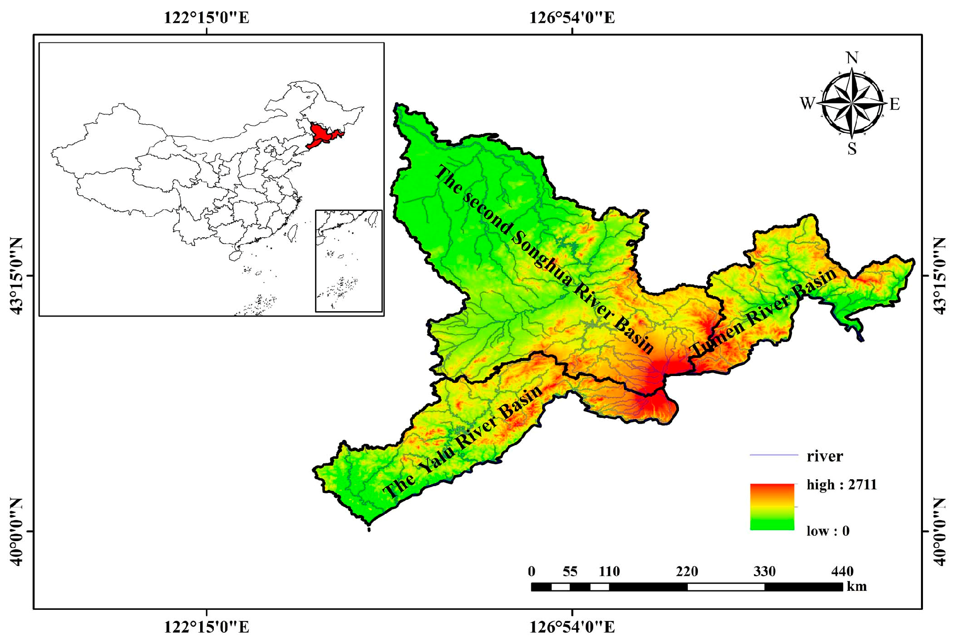
The Changbai Mountain area (N 40°4′47″~45°26′22″, E 123°36′6″~131°14′58″) is located in northeastern China, as shown in Figure 1, and includes the Yalu River, Tumen River and Second Songhua River, covering an area of approximately 127,080 km2. This area is hot and rainy in summer and less rainy and foggy in autumn, with an annual precipitation in the range of approximately 600~900 mm and an annual average temperature of 2.8 °C. The altitude of the study area gradually increases from northwest to southeast. The peak of the area is 2711 m and is located near the Changbai Mountains, where many rivers originate. The entire Changbai Mountain area has a dense water network and numerous rivers.
2.2. Data Sources
2.2.1. Remote Sensing Images
The optical image utilized in this study is Sentinel-2 (https://sentinel.esa.int/web/sentinel/missions/sentinel-2/data-products (accessed on 2 August 2021)), which is composed of two satellites 2A and 2B and has a revisit time of 5 days. Sentinel 2 images have 13 bands, specifically aerosols, blue, green, red, near-infrared and short-wave infrared bands, and their resolutions include 10 m, 20 m and 60 m. They are used for the monitoring of vegetation, soil and water cover, as well as observation of inland waterways and coastal areas. The SAR image is Sentinel-1 IW model data (https://sentinel.esa.int/web/sentinel/missions/sentinel-1/data-products (accessed on 12 September 2021)). Sentinel 1 satellite is composed of A and B satellites and is an active microwave remote sensing satellite with a revisit time of 6 days. The IW mode is the main acquisition mode on land. Satellite images mainly include two intensification modes: VV and VH, which are used to observe land with a resolution of 10 m. The verification data are the Jilin-1 Kuanfu01 (JL-1) satellite data in August 2020 (http://www.jl1.cn/idex.aspx (accessed on 18 September 2021)), which have four bands, specifically blue, green, red and near-infrared, with a resolution of 0.75 m. The parameters of each satellite image are shown in Table 1.
2.2.2. Sample Data
A total of 38,406 samples of water (9248) and non-water (29,158) were selected from the JL-1 satellite image and GF-1 image (http://gaofenplatform.com/channels/45.html (accessed on 25 September 2021)), and 4436 samples were selected using visual interpretation of Sentinel 2 false-color images, as shown in Figure 2. Seventy percent of all samples are used for training, and thirty percent of the sample are used for verification.
2.3. Methodology
The algorithm in this paper is divided into two parts. The first part is the MDFM based on the RF. First, the optical image and SAR image are preprocessed, including the removal of clouds and cloud shadows, filtering, mean synthesis and clip. Second, the water indices are calculated for the optical image; the entropy, contrast and water index are calculated for the SAR image; the above-mentioned parameters serve as the model input; and the known water and non-water sample points are employed as training samples to build an MDFM based on the RF and to generate a water dataset based on the MDFM. The second part is a SWEM based on the MDFM. On the basis of the MDFM dataset, the water boundary was extracted, and buffer analysis was performed to obtain the water boundary. Last, the FCLS method was used to perform superpixel decomposition to construct a model of superpixels based on multisource data fusion and generate a superpixel water dataset based on the SWEM. The flowchart for this article is shown in Figure 3.
2.3.1. Image Preprocessing
The image preprocessing in this paper includes SAR image preprocessing and optical image preprocessing. The process is shown in Figure 4.
(1) Preprocessing of SAR image
The SAR image employed in this paper is the Sentinel-1 ground range detection (GRD) product, which performs boundary noise removal, radiometric calibration, geometric correction and topographic correction [37,38]. Considering the influence of terrain factors on SAR imaging, the tilted terrain is converted to flat terrain based on the relationship between terrain geometry and image parameters, which suppresses the influence of different terrain factors on SAR imaging. In this study, angular-based radiometric slope correction model is used for terrain correction [38]. Due to the coherent imaging mode and scattering characteristic of SAR, some speckles and noise will be generated in the acquisition of ground object information, especially when the ground object background is complex. The speckles and noise will make the gray value of the image more uneven, thus affecting the imaging accuracy of the SAR image. To ensure good image quality, the refined lee filter [39] was applied to the SAR image, which was then clipped to cover the entire study area. The preprocessed image can be used to calculate SAR image parameters and water indices.
(2) Preprocessing of optical image
The optical images used in this study are Sentinel-2 surface reflectance (SR) data, which are radiometrically calibrated and atmospherically corrected and need to be synthesized with the mean value of the images and clipped prior to cloud and cloud shadow removal. First, the images in this period were synthesized with the mean value according to the minimum cloud amount, and the images covered by the study area were clipped out. Second, cloud and cloud shadow removal processing was carried out. In this study, the steps of cloud and cloud shadow removal based on the RF algorithm with multisource data are presented as follows:
- i.
- Using the measured data, 39 clouds, 32 shadows, 23 water bodies and 35 other regions of interest (ROIs) were selected as training labels;
- ii.
- The B1~B12 bands of the optical image and VV and VH of the SAR image were selected as input parameters. Among them, the SAR image is not affected by cloud shadows, and its reflection characteristics are quite different from those of water, so VV and VH can be used to remove cloud shadows;
- iii.
- A RF model was established based on the data (step (i)) to extract clouds and cloud shadows;
- iv.
- Buffer analysis was performed on the clouds and shadows obtained in Step (iii) to achieve cloud removal after deleting the cloud and cloud shadow areas.
(3) Image geometric registration
Considering the different imaging modes and angles of sensors, the same ground object may have position deviation in remote sensing images of multiple sensors. To reduce the error caused by image deviation, it is necessary to carry out geometric registration for multisource remote sensing images. Because Sentinel-1 and Sentinel-2 images have the same sensor, each band is matched at the pixel level. Thus, the registration of the Sentinel-1 image was achieved when JL-1 was registered with Sentinel-2. In this paper, the cross-correlation algorithm was chosen for image registration [40].
2.3.2. MDFM Based on RF
(1) RF algorithm
The RF algorithm is an ensemble classifier constructed using several decision tree models in the bagging integration mode . is an independent random vector with the same distribution. Sample X is input to the RF to obtain the final output . The specific process is described as follows: the training dataset is known, and the sample feature number is m. The bootstrap sampling method is used to extract K datasets with size n from D and to train K decision tree models. In the process of spanning the tree, the dividing node selects or features each time and then selects the most important feature according to the feature evaluation method for node division. The RF algorithm usually integrates K decision tree models in the bagging way and obtains the final result via the majority voting principle or average method [41].
(2) Multi-source data fusion water extraction model
In this paper, the MDFM based on the RF algorithm was constructed; the steps are listed as follows:
- i.
- Water indices of optical images
The water indices of the optical images include NDWI, MNDWI, NDVI, WI 2015, AWEI_sh and AWEI_nsh. The calculation formulas are shown in Table 2.
- ii.
- Water index of the SAR image
The input parameters of the SAR image include entropy, contrast and Sentinel-1 Dual-Polarized Water Index (SDWI). Entropy and contrast are derived from the gray level cooccurrence matrix (GLCM); the formula is expressed as follows:
where is the GLCM, f(x,y) is a remote sensing image, # represents the number of occurrence of point pairs (xi, yi) and (xj, yj), Con is contrast, Ent is entropy, L means that the image has L gray levels, that is, the image dimension is . is the normalized GLCM, which represents the occurrence probability of two pixels with grayscale values of i and j having a certain spatial relation d.
SDWI is a band operation based on the backscattering coefficient of the SAR image to further expand the difference between water bodies and other ground objects. The calculation formula is expressed as follows:
where VV and VH are the backscattering coefficients of the SAR image.
- iii.
- Construction of the MDFM based on the RF
Selecting the water indices calculated in (i) and (ii) and the bands B1~B12 of the optical image, VV and VH of the SAR image, and the DEM serve as input parameters to build a water body extraction model based on the RF. The samples are utilized for training and validation. Among them, B1~B12, VV and VH are used to characterize the water information contained in remote sensing images. Each water index, entropy and contrast are used to suppress the features that are similar to water and enhance the spectral and texture characteristics of water. DEM is used to reduce the influence of ground object shadow and ground objects with similar background for water during optical image imaging, and correct the effects of topography for water extraction.
2.3.3. Water Boundary Extraction
To achieve the superpixel decomposition of the water boundary, the water boundary needs to be extracted. In this study, a canny edge detection algorithm [45] was used to extract the boundary of the water extracted using the MDFM, and then a buffer of two pixels was set for the extracted water boundary to retain more water boundary information. The water boundary can be obtained after the water from the MDFM has been extracted using a buffer.
2.3.4. Super-Pixel Decomposition of Water Boundary
(1) FCLS
When there are mixed pixels in the ground object, the linear spectral mixing model is generally utilized for image unmixing; its formula is expressed as follows:
where X is the remote sensing image, A is the endmember of the image, S is the abundance, and N are the noise and error.
Linear spectral unmixing is usually expanded based on the least square method. When the noise and error are disregarded, solving the abundance S can be transformed into a linear estimation problem:
The conditions of “nonnegative” and “normalization” are added on the basis of the least squares method, and the matrix is constructed as follows:
where 1T represents the column vector with all elements of 1, which is a constant used to control the error. A’ and X’ are substituted for A and X, respectively, and the result is obtained. The least squares algorithm that satisfies both “nonnegativity” and “normalization” is referred to as FCLS [46,47].
(2) SWEM based on multi-source data fusion
Based on the advantages and disadvantages of optical and SAR remote sensing images, the superpixel decomposition of the water boundary is divided into the without clouds situation and with clouds situation. When there are clouds, the optical image is affected by clouds and shadows, which leads to a loss of water boundary data. This part needs to be completed using the SAR image, and then the FCLS method is employed for superpixel decomposition. If there is no cloud in the optical image, the water boundary is decomposed using the optical image.
2.4. Accuracy Evaluation
To measure the accuracy of the algorithm, this paper selects the JL-1 image as the measured data, resamples them to the resolution of the water extraction results, conducts correlation analysis and area statistics with the water extraction results, and uses the correlation coefficient r and water area accuracy Parea for evaluation.
The correlation coefficient r is calculated by:
where r is the correlation coefficient and X and Y are two variables representing the pixel values of water and non-water extracted in this study and the corresponding measured data, respectively. The closer the absolute value of r is to 1, the higher the correlation between the two variables.
The calculation formula of water area accuracy Parea is expressed as follows:
where Parea is the accuracy of the water area, Acal is the calculated water area, and Atrue is the measured area. The closer Parea is to 1, the higher the area accuracy. The calculation process of Acal is expressed as follows:
- i.
- A fishnet was created in the study area based on the pixel size of Sentinel-1 and Sentinel-2 images, and sample labels were created in each grid;
- ii.
- The actual area value represented by the grid was calculated;
- iii.
- The pixel values of each grid were counted using the sample labels in step (i);
- iv.
- The water area can be obtained by accumulating the grid pixel values calculated in step (iii) and multiplying by the grid area in step (ii).
3. Results
3.1. Image Preprocessing Results
Figure 5 shows the images and preprocessing results of the Yinma River, in which Figure 5a is the original Sentinel-2 image. The results obtained after mean synthesis and cloud and cloud shadow removal are shown in Figure 5b. It can be seen that the clouds and cloud shadows in the image are removed to the maximum extent, and the effect is good. Figure 5c is the original image of Sentinel-1. The result after the refined lee filter is shown in Figure 5d, which inhibits speckle noise while preserving the edge information of ground objects. Figure 5e is a false color composite image of the JL-1 image, and the water is obtained as shown in Figure 5f, which is classified using SVM from Figure 5e and utilized for accuracy evaluation.
3.2. Results of Water Extraction of the Multisource Remote Sensing Data Fusion
To compare the results of different data sources, this paper only used optical images, SAR images and multisource data (optical images and SAR images) as inputs and selected the RF algorithm to extract the water bodies of the Yinma River. The optical image can be divided into the without clouds condition and with clouds condition; the results are shown in Figure 6.
The results show that when there is a cloud in the optical image (Figure 6a), water omissions are caused by clouds and cloud shadows covering (red part in the figure). When the optical image does not contain clouds (Figure 6b), the water body extraction effect is good. The boundary of water extracted from the SAR image is relatively complete (Figure 6c) but lacks spectral information, resulting in the loss of some water (marked part in Figure 6c). When there are clouds in the optical image, using multisource data identifies the part that is missed when only the optical image is employed for water extraction (marked part in Figure 6d), fully utilizing the penetrating characteristics of the SAR image. When there are no clouds in the optical image, the water extracted using the MDFM has a good effect (Figure 6e), and the spectral information of the optical image and texture information of the SAR image are fully and simultaneously utilized in this process. The water body results of the JRC-GSWE (Figure 6f) in the same month had many omissions (marked part of Figure 6f) because of data loss caused by clouds, rain, fog, cloud shadows and other factors or insufficient image resolution, which made it difficult to extract small water bodies.
To quantitatively describe the water extraction accuracy, r and Parea were calculated between the above-mentioned water extraction results (Figure 6) and the high-resolution water extraction results of the JL-1 satellite (Figure 5f). The obtained results are shown in Table 3.
As Table 3 shows, when the optical image only served as an input, the correlation coefficients between the without clouds condition and the with clouds condition were 0.90 and 0.54, respectively, and the area accuracies were 0.86 and 0.38, respectively, indicating that clouds have a great influence on the water identification accuracy. When the SAR image only served as an input, the correlation coefficient and area accuracy were 0.78 and 0.63, respectively. Compared with the scenario of using only optical images with clouds, the water recognition result was more complete, with some omissions. The correlation coefficient and area accuracy (r = 0.90 and 0.83; Parea = 0.87 and 0.79, respectively) of water extracted using the MDFM were better than those obtained in the scenario in which only optical and SAR images were utilized (r = 0.90, 0.56, and 0.78; Parea = 0.86, 0.38, and 0.63, respectively) under without clouds and with clouds conditions. The correlation coefficient and area accuracy of the MDFM were also higher than those of the JRC-GSWE (r = 0.65 and Parea = 0.51, respectively) in the same month. This finding shows that the MDFM in this paper has the complementary advantages of optical images and SAR images and can achieve all-weather water extraction and improve the accuracy of water identification.
3.3. Water Extraction in Changbai Mountain area Based on MDFM
Applying the MDFM algorithm to the Changbai Mountain area, the water body results from September 11, 2020, to September 24, 2020, were obtained (Figure 7a). The water body results of the JRC-GSWE in the same month are shown in Figure 7b. The results reveal that the results obtained in this study are generally close to the JRC-GSWE. To further compare the extraction effect of different characteristic water bodies, such as watersheds, reservoirs and streams, watersheds (circles 1 and 2 in Figure 7a), reservoirs (circle 3 in Figure 7a) and streams (circle 4 in Figure 7a) were selected for magnification comparison. The results are shown in Figure 7a-1–c-4.
The results show that the MDFM identified the unrecognized part of the JRC-GSWE (marked in Figure 7b-1) and the disconnected part of the JRC-GSWE (marked in Figure 7b-2). As shown in Figure 7a-1–c-2), the MDFM has a better identification effect than JRC-GSWE in large watersheds, making the water more complete as a whole. As shown in the enlarged effect of the reservoir, the MDFM identified the missing water of the JRC-GSWE (Figure 7b-3). In stream identification, the MDFM recognized the cutoff part (marked part in Figure 7b-4) in the JRC-GSWE identification result. Based on Figure 7a-3–c-4, the MDFM is superior to JRC-GSWE in reservoir and stream identification. In conclusion, the MDFM has better identification results than the JRC-GSWE for large watersheds and small inland water bodies (streams and reservoirs).
3.4. Water Extraction Results of MDFM and SWEM
The water boundary extracted from the MDFM was decomposed using the FCLS method for superpixel decomposition, and the decomposed water results of the Yinma River are shown in Figure 8.
As shown in Figure 8, Figure 8a is the overall decomposition results in the Yinma River Basin. In the case of the no clouds condition, Figure 8b shows the water results of optical image decomposition. After superpixel decomposition of the water boundary, water bodies in small areas and large areas are similar to the measured results. Figure 8c shows the decomposition results of the SAR image in the Yinma River. The SAR image can well decompose the water boundary, and the decomposition effect is weaker than that of the optical image. In the case of clouds, Figure 8d shows the decomposition results of the spliced image of the Yinma River. The light red area represents optical image decomposition, and the light yellow area denotes SAR image decomposition. The water boundary decomposition effect is good in both the optical image decomposition area and the SAR decomposition area, and the pixel value of water gradually decreases outward at the boundary. Figure 8e shows the decomposition results of the SAR image of the Yinma River, which can comprehensively decompose the water boundary. Figure 8f shows the measured results of the water body in the Yinma River. By creating a fishnet, the measured results of subresolution is cut to the same resolution as the optical and SAR images for comparison of the decomposition results.
In this study, the correlation coefficient and accuracy of the water area between the water extraction results and the JL-1 satellite images were calculated. The results are shown in Table 4.
The results shown that in the without clouds condition, the correlation coefficients (r = 0.92 and 0.91, respectively) and area accuracy (Parea = 0.95 and 0.88, respectively) of optical image decomposition and SAR image decomposition are higher than those of the MDFM (r = 0.90 and Parea = 0.87, respectively) and JRC-GSWE (r = 0.65 and Parea = 0.51, respectively), and the water correlation coefficient and area accuracy decomposed with the optical image are higher than the decomposition results obtained using only the SAR image, which also shows that the optical image decomposition effect is superior to that of the SAR images. The reason is that the optical image bands are more abundant and the spectral information is rich, which have obvious advantages for ground object recognition when there are no clouds and can well decompose the water boundary.
In the case of clouds, the correlation coefficient (r = 0.86) and area accuracy (Parea = 0.94, 0.88) of spliced image decomposition and SAR image decomposition exceed the results of the MDFM (r = 0.83 and Parea = 0.79, respectively) and JRC-GSWE (r = 0.65 and Parea = 0.51, respectively). In conclusion, the accuracy of the water extracted using the MDFM and SWEM under the without clouds and with clouds conditions was increased compared with that of the MDFM, which had a higher degree of increase than JRC-GSWE. The water extraction results of the MDFM and SWEM were the best.
3.5. Water Extraction Results of MDFM and SWEM in Changbai Mountain Area
The MDFM and SWEM algorithms were applied to the Changbai Mountain area, and the results are shown in Figure 9. The results show that superpixel decomposition for the water boundary can effectively obtain the water proportion of mixed pixels in the water boundary and improve the accuracy of water extraction. Similarly, the watershed (circles 1 and 2 in Figure 9), reservoir (circle 3 in Figure 9) and stream (circle 4 in Figure 9) were compared on a large scale.
It can be seen from the results that the water proportion of the mixed pixels in water boundary are obtained and reach the super-pixel level. In circle 1 and 2, the super-pixel decomposition of water boundary makes the watershed boundary have layers, as shown in (b-1)–(c-1) and (b-2)–(c-2) of Figure 9. In streams and reservoirs, super-pixel decomposition makes local small water bodies in streams and reservoirs more finely identified, and the boundaries of small water bodies are more complete, as shown in (b-3)–(c-3) and (b-4)–(c-4) in Figure 9.
In summary, MDFM and SWEM have achieved the all-weather, super-pixel extraction of the water body, and have high spatial resolution.
3.6. Temporal Resolution of Water Extraction in the Changbai Mountain Area
To determine the temporal resolution of water extraction, optical and SAR remote sensing images (https://scihub.copernicus.eu/ (accessed on 2 August 2021 and 12 September 2021)) of the study area from 1 September 2020, to 31 October 2020, were counted. The specific date and data synthesis time are shown in Table 5. As shown in Table 5, the water body results covering the whole research area can be obtained by using the algorithm in this paper every 6–13 days, which has a higher temporal resolution than the JRC-GSWE (30 days).
4. Discussion
(1) Influence of input parameters of multisource data fusion on water extraction results
In this study, entropy, contrast, DEM and SDWI were selected as input parameters for SAR images, which effectively solves the problem that SAR image parameters are few and comprise a small proportion in data fusion. The entropy (Figure 10a) and contrast (Figure 10b) are sensitive to the water boundary and their characteristics are more distinct than other ground objects, which has obvious advantages. For optical images, the water features are highlighted to the maximum extent by the water indices of NDWI, MNDWI, AWEI, NDVI and WI 2015 to further improve the accuracy of water extraction.
(2) Influence of different data sources on superpixel decomposition for the water boundary
In this study, there are many clouds and cloud shadows at the water boundary of the Yinma River, which make the optical image account for a relatively small proportion in the spliced image, and the correlation coefficient r of the MDFM and SWEM decomposed using the spliced image is almost equal to that using only the SAR image. However, the area accuracy Parea of the MDFM and SWEM using the spliced image is 6.82% higher than that of only the SAR image, indicating that Parea is more sensitive to water boundary changes than r.
(3) Comparison between MDFM and DL
As an important breakthrough in deep learning, deep belief networks (DBNs) have been widely considered by scholars since they were proposed [48].In recent years, DL has made important breakthroughs in the field of computer vision and has been widely used in surface water mapping as a more advanced method [22,24,49]. An adaptive model based on DL WatNet, is proposed, and combines image classification technology and a semantic segmentation method to establish a global surface water knowledge base composed of satellite images, with high accuracy and stability [5]. In this study, a deep learning water extraction experiment was carried out to compare the accuracy of MDFM and the WatNet algorithm. The results are shown in the Figure 11 and Table 6.
It can be seen from Figure 11 and Table 6, that the water extracted using MDFM in this study is more complete (Figure 11a,b), and there certain flows disconnected and missing in WatNet (Figure 11c,d). At the same time, the accuracy of MDFM between the without clouds condition (r= 0.90, Parea = 0.87) and the with clouds condition (r = 0.83, Parea = 0.79) were both higher than that of WatNet (r = 0.83, Parea = 0.76; r = 0.64, Parea = 0.44, respectively). The reason for Figure 11c is that WatNet uses optical images for water extraction, which is affected by clouds and cloud shadows, resulting in the absence of water extraction. The MDFM fuses of optical and SAR images can better solve the problem. Figure 11d mainly shows that there are many wetlands and buildings on the boundary of water bodies, and the scene is relatively complex. Optical images are easy to cause misclassification and leakage. The fusion of SAR images maximize the accuracy of water body extraction.
(4) Existing problems
First, Sentinel-1 images started in 2014, and Sentinel-2 images started in 2015. Before 2014, there were no Sentinel-1 images, and the time length of the water dataset had certain limitations. In the future, Radarsat, TerraSAR, ALOS-PALSAR and other SAR images and Landsat series satellite images will be employed for multisource data fusion to extract water, and then the extracted water boundary will be decomposed using superpixels to further improve the accuracy of water and to generate a water dataset with a longer interval time series. Second, the validation results of this study were only evaluated for accuracy in the Yinma River. Although both the correlation coefficient and area accuracy are high, there are certain limitations in the validation area. In the future, experiments and accuracy verification will be carried out in several different areas. At the same time, by fusing optical and SAR images, the algorithm in this study can extract water bodies in all-weather conditions and obtain the disaster affected area and distribution of disasters. With high temporal and spatial resolution, it can be used for sudden disaster monitoring and disaster control. Next, we will carry out time series extraction of water bodies, expand the monitoring scope, and further promote the dataset. The evolution of flood disaster in recent decades will be analyzed to provide theoretical basis for further improvement of prevention and control measures.
5. Conclusions
In this study, an all-weather and superpixel water extraction method of the MDMF and SWEM is proposed. The results are presented as the follows:
- (1)
- The correlation coefficient accuracy and area accuracy (r = 0.90 and 0.83; Parea = 0.87 and 0.79, respectively) of the MDFM in the without clouds and with clouds conditions are higher than those when only optical and SAR images were used (r = 0.90, 0.56, and 0.78; Parea = 0.86, 0.38, and 0.63, respectively).
- (2)
- The correlation coefficient and area accuracy of the MDFM and SWEM under the without clouds condition are improved by 2.22% and 9.20%, respectively, compared with the MDFM, and 41.54% and 85.09%, respectively, compared with the JRC-GSWE. The correlation coefficient and area accuracy of the MDFM and SWEM under the with clouds condition are 3.61% and 18.99% higher, respectively, than those of the MDFM and 32.31% and 84.31% higher, respectively, than those of the JRC-GSWE, indicating that the MDFM and SWEM could further improve the accuracy of water extraction.
- (3)
- The water dataset of the Changbai Mountain area is generated every 6~13 days with high temporal resolution.
The algorithm proposed in this paper can achieve all-weather water extraction with high spatiotemporal resolution and has outstanding advantages in monitoring extreme climate disasters and identifying small water bodies such as ponds and reservoirs, which has significance for ensuring the safety of people’s lives and property and for promoting the sustainable development of production and life.
Author Contributions
Conceptualization, methodology, validation, X.C.; data curation, writing—original draft preparation, F.G.; visualization, investigation, Y.L.; software, validation, B.W.; reviewing, guide the experiment, supervision, X.L. All authors have read and agreed to the published version of the manuscript.
Funding
This work was supported by the National Key Research and Development Project of China under Grant 2019YFC0409101.
Data Availability Statement
Not applicable.
Conflicts of Interest
The authors declare no conflict of interest.
References
- Biggs, J.; Von Fumetti, S.; Kelly-Quinn, M. The importance of small waterbodies for biodiversity and ecosystem services: Implications for policy makers. Hydrobiologia 2017, 793, 3–39. [Google Scholar]
- Druce, D.; Tong, X.; Lei, X.; Guo, T.; Kittel, C.M.; Grogan, K.; Tottrup, C. An optical and SAR based fusion approach for mapping surface water dynamics over Mainland China. Remote Sens. 2021, 13, 1663. [Google Scholar] [CrossRef]
- Feyisa, G.L.; Meilby, H.; Fensholt, R.; Proud, S.R. Automated Water Extraction Index: A new technique for surface water mapping using Landsat imagery. Remote Sens. Environ. 2014, 140, 23–35. [Google Scholar] [CrossRef]
- Morss, R.E.; Wilhelmi, O.V.; Downton, M.W.; Gruntfest, E. Flood risk, uncertainty, and scientific information for decision making: Lessons from an interdisciplinary project. Bull. Am. Meteorol. Soc. 2005, 86, 1593–1602. [Google Scholar] [CrossRef]
- Luo, X.; Tong, X.; Hu, Z. An applicable and automatic method for earth surface water mapping based on multispectral images. Int. J. Appl. Earth Obs. Geoinf. 2021, 103, 102472. [Google Scholar] [CrossRef]
- McFeeters, S.K. The use of the Normalized Difference Water Index (NDWI) in the delineation of open water features. Int. J. Remote Sens. 1996, 17, 1425–1432. [Google Scholar] [CrossRef]
- Qiu, J.; Cao, B.; Park, E.; Yang, X.; Zhang, W.; Tarolli, P. Flood monitoring in rural areas of the Pearl River Basin (China) using Sentinel-1 SAR. Remote Sens. 2021, 13, 1384. [Google Scholar] [CrossRef]
- Pohl, C.; Van Genderen, J.L. Review article multisensor image fusion in remote sensing: Concepts, methods and applications. Int. J. Remote Sens. 1998, 19, 823–854. [Google Scholar] [CrossRef] [Green Version]
- Chang, N.-B.; Bai, K.; Imen, S.; Chen, C.-F.; Gao, W. Multisensor satellite image fusion and networking for all-weather environmental monitoring. IEEE Syst. J. 2016, 12, 1341–1357. [Google Scholar] [CrossRef]
- Jiang, X.; Li, G.; Liu, Y.; Zhang, X.-P.; He, Y. Homogeneous transformation based on deep-level features in heterogeneous remote sensing images. In Proceedings of the IGARSS 2019-2019 IEEE International Geoscience and Remote Sensing Symposium, Yokohama, Japan, 28 June–2 July 1999; pp. 106–109. [Google Scholar]
- Zhang, L.; Shen, H. Progress and future of remote sensing data fusion. J. Remote Sens. 2016, 20, 1050–1061. [Google Scholar]
- Zhang, T.; Ren, H.; Qin, Q.; Zhang, C.; Sun, Y. Surface water extraction from Landsat 8 OLI imagery using the LBV transformation. IEEE J. Sel. Top. Appl. Earth Obs. Remote Sens. 2017, 10, 4417–4429. [Google Scholar] [CrossRef]
- Wang, Q.; Blackburn, G.A.; Onojeghuo, A.O.; Dash, J.; Zhou, L.; Zhang, Y.; Atkinson, P.M. Fusion of Landsat 8 OLI and Sentinel-2 MSI data. IEEE Trans. Geosci. Remote Sens. 2017, 55, 3885–3899. [Google Scholar] [CrossRef]
- Tu, T.-M.; Huang, P.S.; Hung, C.-L.; Chang, C.-P. A fast intensity-hue-saturation fusion technique with spectral adjustment for IKONOS imagery. IEEE Geosci. Remote Sens. Lett. 2004, 1, 309–312. [Google Scholar] [CrossRef]
- Yang, Y.; Han, C.; Kang, X.; Han, D. An overview on pixel-level image fusion in remote sensing. In Proceedings of the 2007 IEEE International Conference on Automation and Logistics, Jinan, China, 18–21 August 2007; pp. 2339–2344. [Google Scholar]
- Cakir, H.I.; Khorram, S. Pixel level fusion of panchromatic and multispectral images based on correspondence analysis. Photogramm. Eng. Remote Sens. 2008, 74, 183–192. [Google Scholar] [CrossRef] [Green Version]
- Kulkarni, S.C.; Rege, P.P. Pixel level fusion techniques for SAR and optical images: A review. Inf. Fusion 2020, 59, 13–29. [Google Scholar] [CrossRef]
- Benz, U.C.; Hofmann, P.; Willhauck, G.; Lingenfelder, I.; Heynen, M. Multi-resolution, object-oriented fuzzy analysis of remote sensing data for GIS-ready information. ISPRS J. Photogramm. Remote Sens. 2004, 58, 239–258. [Google Scholar] [CrossRef]
- Sveinsson, J.R.; Ulfarsson, M.O.; Benediktsson, J.A. Cluster-based feature extraction and data fusion in the wavelet domain. In IGARSS 2001. Scanning the Present and Resolving the Future, Proceedings of the IEEE 2001 International Geoscience and Remote Sensing Symposium (Cat. No. 01CH37217), Sydney, NSW, Australia, 9–13 July 2001; IEEE: Piscataway, NJ, USA; 2. [Google Scholar]
- Lehner, B.; Grill, G. Global river hydrography and network routing: Baseline data and new approaches to study the world’s large river systems. Hydrol. Process. 2013, 27, 2171–2186. [Google Scholar] [CrossRef]
- Bonnefon, R.; Dhérété, P.; Desachy, J. Geographic information system updating using remote sensing images. Pattern Recogn. Lett. 2002, 23, 1073–1083. [Google Scholar] [CrossRef]
- Yu, L.; Zhang, R.; Tian, S.; Yang, L.; Lv, Y. Deep multi-feature learning for water body extraction from Landsat imagery. Autom. Control Comput. Sci. 2018, 52, 517–527. [Google Scholar] [CrossRef]
- LeCun, Y.; Bottou, L.; Bengio, Y.; Haffner, P. Gradient-based learning applied to document recognition. Proc. IEEE 1998, 86, 2278–2324. [Google Scholar] [CrossRef] [Green Version]
- Li, M.; Wu, P.; Wang, B.; Park, H.; Yang, H.; Wu, Y. A deep learning method of water body extraction from high resolution remote sensing images with multisensors. IEEE J. Sel. Top. Appl. Earth Obs. Remote Sens. 2021, 14, 3120–3132. [Google Scholar] [CrossRef]
- Li, J.; Ma, R.; Cao, Z.; Xue, K.; Xiong, J.; Hu, M.; Feng, X. Satellite Detection of Surface Water Extent: A Review of Methodology. Water 2022, 14, 1148. [Google Scholar] [CrossRef]
- Saghafi, M.; Ahmadi, A.; Bigdeli, B. Sentinel-1 and Sentinel-2 data fusion system for surface water extraction. J. Appl. Remote Sens. 2021, 15, 014521. [Google Scholar] [CrossRef]
- Challa, S.; Koks, D. Bayesian and dempster-shafer fusion. Sadhana 2004, 29, 145–174. [Google Scholar] [CrossRef]
- Fauvel, M.; Chanussot, J.; Benediktsson, J.A. Decision fusion for the classification of urban remote sensing images. IEEE Trans. Geosci. Remote Sens. 2006, 44, 2828–2838. [Google Scholar] [CrossRef]
- Benediktsson, J.A.; Kanellopoulos, I. Classification of multisource and hyperspectral data based on decision fusion. IEEE Trans. Geosci. Remote Sens. 1999, 37, 1367–1377. [Google Scholar] [CrossRef] [Green Version]
- Pickens, A.H.; Hansen, M.C.; Hancher, M.; Stehman, S.V.; Tyukavina, A.; Potapov, P.; Marroquin, B.; Sherani, Z. Mapping and sampling to characterize global inland water dynamics from 1999 to 2018 with full Landsat time-series. Remote Sens. Environ. 2020, 243, 111792. [Google Scholar] [CrossRef]
- Downing, J.A.; Cole, J.J.; Duarte, C.; Middelburg, J.J.; Melack, J.M.; Prairie, Y.T.; Kortelainen, P.; Striegl, R.G.; McDowell, W.H.; Tranvik, L.J. Global abundance and size distribution of streams and rivers. Inland Waters 2012, 2, 229–236. [Google Scholar] [CrossRef]
- Kristensen, P.; Globevnik, L. European small water bodies. Biol. Environ. Proc. R. Ir. Acad. 2014, 114, 281–287. [Google Scholar] [CrossRef]
- Carroll, M.L.; Townshend, J.R.; DiMiceli, C.M.; Noojipady, P.; Sohlberg, R.A. A new global raster water mask at 250 m resolution. Int. J. Digit. Earth 2009, 2, 291–308. [Google Scholar] [CrossRef]
- Yamazaki, D.; Sato, T.; Kanae, S.; Hirabayashi, Y.; Bates, P.D. Regional flood dynamics in a bifurcating mega delta simulated in a global river model. Geophys. Res. Lett. 2014, 41, 3127–3135. [Google Scholar] [CrossRef] [Green Version]
- Lehner, B.; Verdin, K.; Jarvis, A. New global hydrography derived from spaceborne elevation data. Eos Trans. Am. Geophys. Union 2008, 89, 93–94. [Google Scholar] [CrossRef]
- Aires, F.; Prigent, C.; Fluet-Chouinard, E.; Yamazaki, D.; Papa, F.; Lehner, B. Comparison of visible and multi-satellite global inundation datasets at high-spatial resolution. Remote Sens. Environ. 2018, 216, 427–441. [Google Scholar] [CrossRef] [Green Version]
- Mullissa, A.; Vollrath, A.; Odongo-Braun, C.; Slagter, B.; Balling, J.; Gou, Y.; Gorelick, N.; Reiche, J. Sentinel-1 sar backscatter analysis ready data preparation in google earth engine. Remote Sens. 2021, 13, 1954. [Google Scholar] [CrossRef]
- Vollrath, A.; Mullissa, A.; Reiche, J. Angular-based radiometric slope correction for Sentinel-1 on google earth engine. Remote Sens. 2020, 12, 1867. [Google Scholar] [CrossRef]
- Lee, J.-S. Refined filtering of image noise using local statistics. Comput. Graph. Image Process. 1981, 15, 380–389. [Google Scholar] [CrossRef]
- Pratt, W.K. Correlation techniques of image registration. IEEE Trans. Aerosp. Electron. Syst. 1974, 3, 353–358. [Google Scholar] [CrossRef]
- Gislason, P.O.; Benediktsson, J.A.; Sveinsson, J.R. Random forests for land cover classification. Pattern Recognit. Lett. 2006, 27, 294–300. [Google Scholar] [CrossRef]
- Xu, H. Modification of normalised difference water index (NDWI) to enhance open water features in remotely sensed imagery. Int. J. Remote Sens. 2006, 27, 3025–3033. [Google Scholar] [CrossRef]
- Crippen, R.E. Calculating the vegetation index faster. Remote Sens. Environ. 1990, 34, 71–73. [Google Scholar] [CrossRef]
- Fisher, A.; Flood, N.; Danaher, T. Comparing Landsat water index methods for automated water classification in eastern Australia. Remote Sens. Environ. 2016, 175, 167–182. [Google Scholar] [CrossRef]
- Canny, J. A computational approach to edge detection. IEEE Trans. Pattern Anal. Mach. Intell. 1986, 6, 679–698. [Google Scholar] [CrossRef]
- Heinz, D.; Chang, C.-I.; Althouse, M.L. Fully constrained least-squares based linear unmixing [hyperspectral image classification]. In Proceedings of the IEEE 1999 International Geoscience and Remote Sensing Symposium. IGARSS’99 (Cat. No. 99CH36293), Hamburg, Germany, 28 June–2 July 1999; IEEE: Piscataway, NJ, USA, 1999; 2, pp. 1401–1403. [Google Scholar]
- Wang, L.; Liu, D.; Wang, Q. Geometric method of fully constrained least squares linear spectral mixture analysis. IEEE Trans. Geosci. Remote Sens. 2012, 51, 3558–3566. [Google Scholar] [CrossRef]
- Hinton, G.E. Reducing the Dimensionality of Data with Neural Networks. Science 2006, 313, 504–507. [Google Scholar] [CrossRef] [PubMed] [Green Version]
- LeCun, Y.; Bengio, Y.; Hinton, G. Deep learning. Nature 2015, 521, 436–444. [Google Scholar] [CrossRef]
Figure 1.
Study area.

Figure 2.
Sample points.

Figure 3.
Flow chart of MDFM and SWEM.

Figure 4.
Image preprocessing.

Figure 5.
Image and preprocessing results of the Yinma River. (a) Sentinel-2 original image. (b) Preprocessing results of the Figure (a). (c) Sentinel-1 original image. (d)Preprocessing results of the Figure (c). (e) False color composite image. (f) Water body results of the JL-1 image.
Figure 5.
Image and preprocessing results of the Yinma River. (a) Sentinel-2 original image. (b) Preprocessing results of the Figure (a). (c) Sentinel-1 original image. (d)Preprocessing results of the Figure (c). (e) False color composite image. (f) Water body results of the JL-1 image.

Figure 6.
Water extraction results for the Yinma River Basin. (a) Water results extracted from optical image (with clouds). (b) Water results extracted from optical image (without clouds). (c) Water results extracted from SAR image. (d) Water results extracted using the MDFM (with clouds). (e) Water results extracted using the MDFM (without clouds). (f) Water extraction results of JRC-GSWE.

Figure 7.
Water extraction results and enlarged view of water extraction results for the Changbai Mountain area. (a) Water results using the MDFM. (b) Water results of JRC-GSWE. (a-1–a-4) False color image of the circle 1 to circle 4. (b-1–b-4) JRC-GSWE water results of the circle 1 to circle 4. (c-1–c-4) Water results using the MDFM from circle 1 to circle 4.

Figure 8.
Decomposition results for the Yinma River Basin. (a) The overall decomposition results in the Yinma River Basin. (b) Decomposition results of the optical image in the Yinma River (without clouds). (c) Decomposition results of the SAR image in the Yinma River (without clouds). (d) Decomposition results of the spliced image in the Yinma River. (e) Decomposition results of the SAR image in the Yinma River (with clouds). (f) Measured water map of the Yinma River.

Figure 9.
Water map of superpixel decomposition and the results of water decomposition at a larger scale in the Changbai Mountain area. (a) Water results using the SWEM. (a-1–a-4) False color image of circle 1 to circle 4. (b-1–b-4) Water results using the MDFM and SWEM from circle 1 to circle 4. (c-1–c-4) Enlarged water results using the MDFM and SWEM from circle 1 to circle 4. (d-1–d-4) Enlarged water results using the MDFM from circle 1 to circle 4.

Figure 10.
Entropy and contrast of the SAR image. (a) Entropy image. (b) Contrast image.

Figure 11.
The comparison between MDFM and WatNet. (a) Water map using MDFM (with clouds). (b) Water map using MDFM (without clouds). (c) Water map using WatNet (with clouds). (d) Water map using WatNet (without clouds).
Figure 11.
The comparison between MDFM and WatNet. (a) Water map using MDFM (with clouds). (b) Water map using MDFM (without clouds). (c) Water map using WatNet (with clouds). (d) Water map using WatNet (without clouds).


Table 1.
Spectral bands for the JL-1 satellite.
| Band | Band Name | Wavelength Range (nm) | Resolution (m) |
|---|---|---|---|
| B1 | Blue | 450~510 | 0.75 |
| B2 | Green | 510~580 | 0.75 |
| B3 | Red | 630~690 | 0.75 |
| B4 | NIR | 770~895 | 0.75 |
Table 2.
Water indexes of the optical image.
| Name | Abbreviation | Equation | Reference |
|---|---|---|---|
| Normalized difference water index | NDWI | [6] | |
| Modified normalized difference water index | MNDWI | [42] | |
| Normalized difference vegetation index | NDVI | [43] | |
| Automated water extraction index (1) | AWEI_sh | [3] | |
| Automated water extraction index (2) | AWEI_nsh | [2] | |
| Water index 2015 | WI 2015 | [44] |
Note: GREEN is the reflectance of the green band; NIR is the reflectance of the near infrared band; BLUE is the reflectance of the blue band; SWIR, SWIR1 and SWIR2 are the reflectance of shortwave infrared bands; and RED is the reflectance of the red band in Sentinel-2 images. AWEI_nsh and AWEI_sh are both automated water body extraction indices, wherein AWEI_nsh applies to areas without shadow, and AWEI_sh applies to distinguish and eliminate ground objects with backgrounds similar to water bodies [3].
Table 3.
Accuracy of water extraction results in different images.
| Category | r | Parea | |
|---|---|---|---|
| Without clouds | Optical image only | 0.90 | 0.86 |
| MDFM | 0.90 | 0.87 | |
| With clouds | Optical image only | 0.56 | 0.38 |
| MDFM | 0.83 | 0.79 | |
| SAR image only | 0.78 | 0.63 | |
| JRC-GSWE | 0.65 | 0.51 | |
Table 4.
Water extraction accuracy in the Yinma River.
| Category | r | Increase of r | Parea | Increase of Parea | |
|---|---|---|---|---|---|
| Without clouds | MDFM | 0.90 | / | 0.87 | / |
| (MDFM and SWEM)_MDFM (Optical image decomposition) | 0.92 | 2.22% | 0.95 | 9.20% | |
| (MDFM and SWEM)_ JRC-GSWE (Optical image decomposition) | 0.92 | 41.54% | 0.95 | 85.09% | |
| (MDFM and SWEM)_MDFM (SAR image decomposition) | 0.91 | 1.11% | 0.88 | 1.15% | |
| (MDFM and SWEM)_ JRC-GSWE (SAR image decomposition) | 0.91 | 40.00% | 0.88 | 72.55% | |
| With clouds | MDFM | 0.83 | / | 0.79 | / |
| (MDFM and SWEM)_MDFM (Spliced image decomposition) | 0.86 | 3.61% | 0.94 | 18.99% | |
| (MDFM and SWEM)_ JRC-GSWE (Spliced image decomposition) | 0.86 | 32.31% | 0.94 | 84.31% | |
| (MDFM and SWEM)_MDFM (SAR image decomposition) | 0.86 | 3.61% | 0.88 | 11.39% | |
| (MDFM and SWEM)_ JRC-GSWE (SAR image decomposition) | 0.86 | 32.31% | 0.88 | 72.55% | |
| JRC-GSWE | 0.65 | / | 0.51 | / | |
Note: (MDFM+SWEM) _MDFM refers to the comparison with the results of the MDFM, and (MDFM+SWEM) _ JRC-GSWE refers to the comparison with the results of JRC-GSWE.
Table 5.
Image synthesis table for the Changbai Mountain area.
| The Serial Number | Image Type | The Time Interval | Revisit Time /Days | Minimum Image Synthesis Time/Days | Number of Images | The Date of Indispensable Image |
|---|---|---|---|---|---|---|
| 1 | Optical image | 2020.09.03–2020.09.08 | 5 | 5 | 64 | / |
| SAR image | 2020.09.05–2020.09.11 | 6 | 6 | 12 | 2020.09.05 | |
| 2 | Optical image | 2020.09.08–2020.09.13 | 5 | 5 | 63 | / |
| SAR image | 2020.09.11–2020.09.24 | 6 | 13 | 22 | 2020.09.11 | |
| 3 | Optical image | 2020.09.13–2020.09.18 | 5 | 5 | 64 | / |
| SAR image | 2020.09.24–2020.10.06 | 6 | 12 | 20 | 2020.10.05 | |
| 4 | Optical image | 2020.09.18–2020.09.23 | 5 | 5 | 64 | / |
| SAR image | 2020.10.06–2020.10.18 | 6 | 12 | 20 | 2020.10.17 | |
| 5 | Optical image | 2020.09.23–2020.09.28 | 5 | 5 | 70 | / |
| SAR image | 2020.10.18–2020.10.30 | 6 | 12 | 20 | 2020.10.29 |
Table 6.
Water extraction accuracy table of WatNet and MDFM.
| Category | r | Parea | |
|---|---|---|---|
| Without clouds | Optical image only | 0.90 | 0.86 |
| MDFM | 0.90 | 0.87 | |
| WatNet | 0.83 | 0.76 | |
| With clouds | Optical image only | 0.56 | 0.38 |
| MDFM | 0.83 | 0.79 | |
| WatNet | 0.64 | 0.44 | |
| SAR image only | 0.78 | 0.63 | |
| JRC-GSWE | 0.65 | 0.51 | |
Publisher’s Note: MDPI stays neutral with regard to jurisdictional claims in published maps and institutional affiliations. |
© 2022 by the authors. Licensee MDPI, Basel, Switzerland. This article is an open access article distributed under the terms and conditions of the Creative Commons Attribution (CC BY) license (https://creativecommons.org/licenses/by/4.0/).
Share and Cite
MDPI and ACS Style
Chen, X.; Gao, F.; Li, Y.; Wang, B.; Li, X. All-Weather and Superpixel Water Extraction Methods Based on Multisource Remote Sensing Data Fusion. Remote Sens. 2022, 14, 6177. https://doi.org/10.3390/rs14236177
AMA Style
Chen X, Gao F, Li Y, Wang B, Li X. All-Weather and Superpixel Water Extraction Methods Based on Multisource Remote Sensing Data Fusion. Remote Sensing. 2022; 14(23):6177. https://doi.org/10.3390/rs14236177
Chicago/Turabian StyleChen, Xiaopeng, Fang Gao, Yingye Li, Bin Wang, and Xiaojie Li. 2022. "All-Weather and Superpixel Water Extraction Methods Based on Multisource Remote Sensing Data Fusion" Remote Sensing 14, no. 23: 6177. https://doi.org/10.3390/rs14236177
Note that from the first issue of 2016, this journal uses article numbers instead of page numbers. See further details here.