


Estimation of Water Use in Center Pivot Irrigation Using Evapotranspiration Time Series Derived by Landsat: A Study Case in a Southeastern Region of the Brazilian Savanna

Abstract
:
1. Introduction
2. Study Area and Datasets
2.1. Study Area
2.2. Datasets
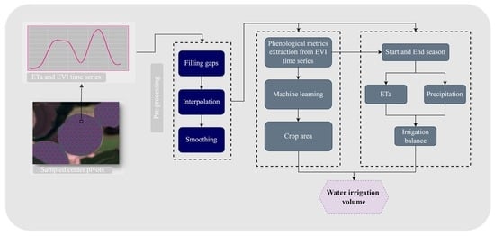
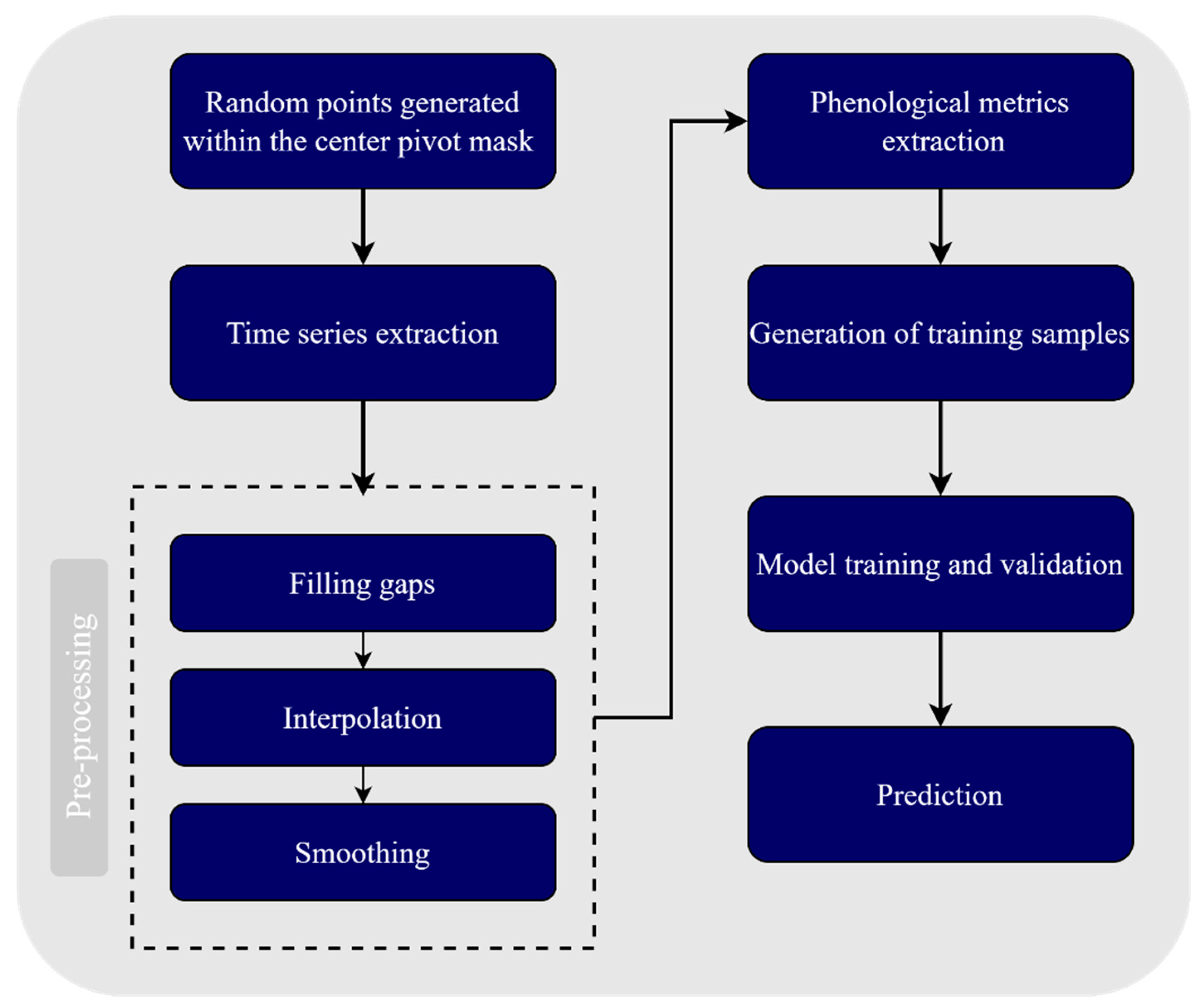
3. Methods
3.1. Crop Classification and Phenological Metrics
3.2. ETa Estimation and SSEBop-Br Assessment
3.3. Irrigation Balance and Water Use
4. Results
4.1. SSEBop-Br Assessment
4.2. Crop Mapping and Area Estimates
4.3. Water Use
4.3.1. Summer Crop Season
4.3.2. Second/Winter Season
4.3.3. Total Water Volume Used in the Center Pivots
5. Discussion
6. Conclusions
Supplementary Materials
Author Contributions
Funding
Acknowledgments
Conflicts of Interest
References
- Agência Nacional de Águas. Atlas Irrigação: Uso Da Água Na Agricultura Irrigada, 2nd ed.; Agência Nacional de Águas: Brasilia, Brazil, 2021; p. 130.
- Agência Nacional de Águas. Polos Nacionais De Agricultura Irrigada; Agência Nacional de Águas: Brasilia, Brazil, 2020; p. 26.
- Dalin, C.; Taniguchi, M.; Green, T.R. Unsustainable Groundwater Use for Global Food Production and Related International Trade. Glob. Sustain. 2019, 2, e12. [Google Scholar] [CrossRef] [Green Version]
- Davis, K.F.; Rulli, M.C.; Garrassino, F.; Chiarelli, D.; Seveso, A.; D’odorico, P. Water Limits to Closing Yield Gaps. Adv. Water Resour. 2017, 99, 67–75. [Google Scholar] [CrossRef] [Green Version]
- Getirana, A.C.V.; Malta, V.F. Decision Process in a Water Use Conflict in Brazil. Water Resour. Manag. 2020, 22, 103–118. [Google Scholar] [CrossRef]
- Xu, C.; Gong, L.; Jiang, T.; Chen, D.; Singh, V.P. Analysis of spatial distribution and temporal trend of reference evapotranspiration and pan evaporation in Changjiang (Yangtze River) catchment. J. Hydrol. 2006, 327, 81–93. [Google Scholar] [CrossRef]
- Bhattarai, N.; Wagle, P. Recent Advances in Remote Sensing of Evapotranspiration. Remote Sens. 2021, 13, 4260. [Google Scholar] [CrossRef]
- Wanniarachchi, S.; Sarukkalige, R. A Review on Evapotranspiration Estimation in Agricultural Water Management: Past, Present, and Future. Hydrology 2022, 9, 123. [Google Scholar] [CrossRef]
- Schauer, M.; Senay, G.B. Characterizing crop water use dynamics in the Central Valley of California using Landsat-derived evapotranspiration. Remote Sens. 2019, 11, 1782. [Google Scholar] [CrossRef] [Green Version]
- Mhawej, M.; Faour, G. Open-source Google Earth Engine 30-m evapotranspiration rates retrieval: The SEBALIGEE system. Environ. Model. Softw. 2020, 133, 104845. [Google Scholar] [CrossRef]
- Agência Nacional de Águas. Estimativa De Evapotranspiração Real Sensoriamento Remoto No Brasil; Agência Nacional de Águas: Brasilia, Brasil, 2020; p. 41.
- Casassola, A. Caracterização da Atividade Agrícola de Pivôs Centrais Por Meio de Séries Temporais de Imagens Sentinel-2 para Estimativas de Uso da Água na Agricultura Irrigada. Master’s Thesis, Instituto Nacional de Pesquisas Espaciais, São José dos Campos, Brazil, 2022. [Google Scholar]
- Rudorff, B.F.T.; Aguiar, D.A.; Silva, W.F.; Sugawara, L.M.; Adami, M.; Moreira, M.A. Studies on the rapid expansion of sugarcane for ethanol production in São Paulo State (Brazil) using landsat data. Remote Sens. 2010, 2, 1057–1076. [Google Scholar] [CrossRef] [Green Version]
- Borges, E.F.; Sano, E.E. Séries temporais de EVI do MODIS para o mapeamento de uso e cobertura vegetal do oeste da Bahia. Bol. Cienc. Geod. 2014, 20, 526–547. [Google Scholar] [CrossRef]
- Gusso, A.; Formaggio, A.R.; Rizzi, R.; Adami, M.; Rudorff, B.F.T. Soybean crop area estimation by Modis/Evi data. Pesq. Agropec. Bras. 2012, 47, 425–435. [Google Scholar] [CrossRef] [Green Version]
- Arvor, D.; Jonathan, M.; Meirelles, M.S.O.P.; Dubreuil, V.; Durieux, L. Classification of MODIS EVI time series for crop mapping in the state of Mato Grosso, Brazil. Int. J. Remote Sens. 2011, 32, 7847–7871. [Google Scholar] [CrossRef]
- Victoria, D.C.; Paz, A.R.; Coutinho, A.C.; Kastens, J.; Brown, J.C. Cropland area estimates using Modis NDVI time series in the state of Mato Grosso, Brazil. Pesquisa Agropecuária Brasileira. 2012, 47, 1270–1278. [Google Scholar] [CrossRef]
- Bendini, H.N. Agricultural land classification based on phenological information from dense time-series Landsat-like images in the Brazilian Cerrado. Ph.D.’s Thesis, Instituto Nacional de Pesquisas Espaciais, São José dos Campos, Brazil, 2018. [Google Scholar]
- Bendini, H.N.; Garcia Fonseca, L.M.; Schwieder, M.; Korting, T.S.; Sanches, I.A.; Leitão, P.J.; Hostert, P. Detailed agricultural land classification in the Brazilian cerrado based on phenological information from dense satellite image time series. Int. J. Appl. Earth Obs. Geoinf. 2019, 82, 101872. [Google Scholar]
- Senay, G.B. Satellite psychrometric formulation of the Operational Simplified Surface Energy Balance (SSEBop) model for quantifying and mapping evapotranspiration. Appl. Eng. Agric. 2018, 34, 555–566. [Google Scholar] [CrossRef] [Green Version]
- Walter, I.A.; Allen, R.G.; Elliott, R.; Jensen, M.E.; Itenfisu, D.; Mecham, B.; Howell, T.A.; Snyder, R.; Brown, P.; Echings, S.; et al. ASCE’s standardized reference evapotranspiration equation. In Proceedings of the Watershed Management and Operations Management 2000, Fort Collins, CO, USA, 20–24 June 2000; pp. 1–11. [Google Scholar]
- Senay, G.B.; Bohms, S.; Singh, R.K.; Gowda, P.H.; Velpuri, N.M.; Alemu, H.; Verdin, J.P. Operational Evapotranspiration Mapping Using Remote Sensing and Weather Datasets: A New Parameterization for the SSEB Approach. J. Am. Water Resour. Assoc. 2013, 49, 577–591. [Google Scholar] [CrossRef] [Green Version]
- Setzer, J. Atlas Climatológico E Ecológico Do Estado De São Paulo; Comissão Interestadual da Bacia Paraná-Uruguai: São Paulo, Brazil, 1966; p. 61. [Google Scholar]
- Cabral, O.M.R.; Rocha, H.R.; Gash, J.H.; Ligo, M.A.V.; Tatsch, J.D.; Freitas, H.C.; Brasilio, E. Water use in a sugarcane plantation. GCB Bioenergy 2012, 4, 555–565. [Google Scholar] [CrossRef] [Green Version]
- Comitê Da Bacia Do Pardo. Deliberação CBH-PARDO 009/05, Governo do Estado de São Paulo, São Paulo, SP, Brasil. Ribeirão Preto. 2005. Available online: https://sigrh.sp.gov.br/public/uploads/deliberation//3632/009-declara-critica-a-bacia-do-ribeirao-das-congonhas.htm (accessed on 11 November 2021).
- Liu, H.Q.; Huete, A. Feedback based modification of the NDVI to minimize canopy background and atmospheric noise. IEEE Trans. Geosci. Remote. Sens. 1995, 33, 457–465. [Google Scholar] [CrossRef]
- Rufin, P.; Frantz, D.; Ernst, S.; Rabe, A.; Griffiths, P.; Özdoğan, M.; Hostert, P. Mapping cropping practices on a national scale using intra-annual Landsat time series binning. Remote Sens. 2019, 11, 232. [Google Scholar] [CrossRef] [Green Version]
- Tatsch, J.D. Uma Análise dos Fluxos de Superfície e do Microclima Sobre Cerra, Cana-de-Açúcar e Eucalipto, com Implicações para Mudanças Climáticas Regionais. Master’s Thesis, Universidade de São Paulo, São Paulo, Brazil, 2006. [Google Scholar]
- Twine, T.E.; Kustas, W.P.; Norman, J.M.; Cook, D.R.; Houser, P.R.; Meyers, T.P.; Prueger, J.H.; Starks, P.J.; Wesely, M.L. Correcting eddycovariance flux underestimates over a grassland. Agric. Meteorol. 2000, 103, 279–300. [Google Scholar] [CrossRef] [Green Version]
- De la Fuente-Sáiz, D.; Ortega-Farías, S.; Fonseca, D.; Ortega-Salazar, S.; Kilic, A.; Allen, R. Calibration of metric model to estimate energy balance over a drip-irrigated apple orchard. Remote Sens. 2017, 9, 670. [Google Scholar] [CrossRef]
- Oliveira, B.S. Otimização do modelo Metric para estimativas de evapotranspiração no Cerrado brasileiro. Ph.D.’s Thesis, Instituto Nacional de Pesquisas Espaciais, São José dos Campos, Brazil, 2018. [Google Scholar]
- Irmak, S.; Haman, D.Z. Evapotranspiration: Potential or Reference? Department of Agricultural and Biological Engineering- UF/IFAS Extension: Gainesville, FL, USA, 2017; p. 2. [Google Scholar]
- Sanches, I.D.; Feitosa, R.Q.; Diaz, P.M.A.; Soares, M.D.; Luiz, A.J.B.; Schults, B.; Maurano, L.E.P. Campo Verde Database: Seeking to Improve Agricultural Remote Sensing of Tropical Areas. IEEE Geosci. Remote Sens. Lett. 2018, 15, 369–373. [Google Scholar] [CrossRef]
- Soares, A.R.; Bendini, H.N.; Vaz, D.V.; Uehara, T.D.T.; Neves, A.K.; Lechler, S.; Korting, T.S.; Fonseca, L.M.G. STMETRICS: A Python Package for Satellite Image Time-Series Feature Extraction. In Proceedings of the IGARSS 2020: 2020 IEEE International Geoscience and Remote Sensing Symposium, Virtual Symposium, Virtual Symposium, 26 September 2020–2 October 2020. [Google Scholar]
- Jönsson, P.; Eklundh, L. TIMESAT—A program for analyzing time-series of satellite sensor data. Comput. Geosci. 2004, 30, 833–845. [Google Scholar] [CrossRef] [Green Version]
- Jönsson, P.; Eklundh, L. TIMESAT 3.2 with Parallel Processing Software Manual; Lund University: Lund, Sweden, 2015; pp. 22–24. [Google Scholar]
- Harvey, A.C. Forecasting, Structural Time Series Models and the Kalman Filter; Cambridge University Press: Cambridge, UK, 1990. [Google Scholar]
- Dougherty, R.L.; Edelman, A.S.; Hyman, J.M. Nonnegativity-, monotonicity-, or convexity-preserving cubic and quintic Hermite interpolation. Math. Comput. 1989, 52, 471–494. [Google Scholar] [CrossRef]
- Breiman, L. Random Forests. Mach. Learn. 2001, 45, 5–32. [Google Scholar] [CrossRef] [Green Version]
- Liaw, A.; Wiener, M. Classification and regression by randomforest. R. News 2002, 2, 18–22. [Google Scholar]
- Belgiu, M.; Dragut, L. Random Forest in remote sensing: A review of applications and future directions. ISPRS J. Photogramm. Remote Sens. 2016, 114, 24–31. [Google Scholar] [CrossRef]
- Rubinstein, R.; Kroese, D. Simulation and the Monte Carlo Method, 3rd ed.; Wiley—Interscience: Hoboken, NJ, USA, 2008; pp. 1–340. [Google Scholar]
- Chinchor, N.; Sundheim, B. MUC-5 evaluation metrics. In Proceedings of the 5th Conference on Message Understanding, Stroudsburg, PA, USA, 25–27 August 1993. [Google Scholar]
- Shapiro, D.E. The interpretation of diagnostic tests. Stat. Methods Med. Res. 1999, 8, 113–134. [Google Scholar] [CrossRef]
- Xavier, A.C.; King, C.W.; Scanlon, B.R. Daily gridded meteorological variables in Brazil (1980–2013). Int. J. Climatol. 2016, 36, 2644–2659. [Google Scholar] [CrossRef] [Green Version]
- Senay, G.B.; Friedrichs, M.; Singh, R.K.; Velpuri, N.M. Evaluating Landsat 8 evapotranspiration for water use mapping in the Colorado River Basin. Remote Sens. Environ. 2016, 185, 171–185. [Google Scholar] [CrossRef] [Green Version]
- Willmott, C.J.; Matsuura, K. Advantages of the mean absolute error (MAE) over the root mean square error (RMSE) in assessing average model performance. Clim. Res. 2005, 30, 79–82. [Google Scholar] [CrossRef]
- Sorooshian, S.; Duan, Q.; Gupta, V.K. Calibration of rainfall-runoff models: Application of global optimization to the Sacramento Soil Moisture Accounting Model. Water Resour. Res. 1993, 29, 1185–1194. [Google Scholar] [CrossRef]
- Willmott, C.J. On the validation of models. Phys. Geogr. 1981, 2, 184–194. [Google Scholar] [CrossRef]
- Nash, J.E.; Sutcliffe, J.V. River flow forecasting through conceptual models. Part 1: A discussion of principles. J. Hydrol. 1970, 10, 282–290. [Google Scholar] [CrossRef]
- Van Liew, M.W.; Veith, T.L.; Bosch, D.D.; Arnold, J.G. Suitability of SWAT for the Conservation effects assessment project: A comparison on USDA-ARS watersheds. J. Hydrol. Eng. 2007, 12, 173–189. [Google Scholar] [CrossRef] [Green Version]
- Agência Nacional de Águas; National Institute for Space Research. Colaboração ANA-INPE Para O Atlas Irrigação 2021: Monitoramento De Pivôs Centrais Nos Polos De Agricultura Irrigada Do Cerrado; Nota Técnica Conjunta, Nº 3/2021/SPR/INPE; Agência Nacional de Águas (ANA), Ed.; Agência Nacional de Águas (ANA): Brasília, Brazil, 2021.
- Naghedifar, S.M.; Ziaei, A.N.; Ansari, H. Simulation of irrigation return flow from a Triticale farm under sprinkler and furrow irrigation systems using experimental data: A case study in arid region. Agric. Water Manag. 2018, 210, 185–197. [Google Scholar] [CrossRef]
- Silveira, J.M.d.C.; Lima Júnior, S.d.; Sakai, E.; Matsura, E.E.; Pires, R.C.d.M.; Rocha, A.M. Identificação de áreas irrigadas por pivô central na sub-bacia tambaú-verde utilizando imagens ccd/cbers. Irriga 2013, 18, 721–729. [Google Scholar] [CrossRef] [Green Version]
- Radin, B. Evapotranspiração máxima do milho medida em lisímetro e estimada pelo modelo de Penman-Monteith modificado. Master’s Thesis, Federal University of Rio Grande do Sul, Porto Alegre, Brazil, 1998. [Google Scholar]
- Alves, É.S. Evapotranspiração atual da cultura de soja: Modelagem e avaliação da evaporação direta da água do solo. Ph.D. Thesis, Universidade Federal de Viçosa, Viçosa, Brazil, 2020. [Google Scholar]
- Allen, R.G.; Pereira, L.S.; Raes, D.; Smith, M. Crop Evapotranspiration—Guidelines for Computing Crop Water Requirements; FAO Irrigation and Drainge: Rome, Italy, 1998; p. 56. [Google Scholar]
- EMBRAPA. Tecnologias De Produção De Soja: Região Central Do Brasil, 2001; Embrapa Soja: Londrina, Brazil, 2002; p. 199. [Google Scholar]
- EMBRAPA. Tecnologias De Produção De Soja—Região Central Do Brasil; Embrapa Cerrados: Planaltina, Brazil, 2011; p. 21. [Google Scholar]
- Lunardi, D.M.C.; Filho, J.L. Evapotranspiração máxima e coeficiente de cultura da cenoura (Daucus carota L.). Rev. Bras. Agrometeorol. 1999, 7, 13–17. [Google Scholar]
- Moura, M.V.T.; Marques Júnior, S.; Brotel, T.A.; Frizone, J.A. Estimativa do consumo de água da cultura da cenoura (Daucus carota, L.) v. Nantes Superior, para a região de Piracicaba, através do Balanço Hídrico. Sci. Agric. 1994, 51, 284–291. [Google Scholar] [CrossRef] [Green Version]
- EMBRAPA. Irrigação Da Cultura Da Cenoura (Circular Técnica, 48); Embrapa Hortaliças: Brasília, Brazil, 2007; p. 14. [Google Scholar]
- Matzenauer, R.; Maluf, J.R.T.; Bueno, A.C. Evapotranspiração da cultura do feijão e sua relação com a evaporação do tanque classe "A”. Pesqui. Agropecuária Gaúcha 1998, 4, 101–106. [Google Scholar]
- EMBRAPA. Conhecendo A Fenologia Do Feijoeiro E Seus Aspectos Fitotécnicos; Embrapa Arroz e Feijão: Brasilia, Brazil, 2018; p. 59. [Google Scholar]
- EMBRAPA. Irrigação Na Cultura Da Cebola, (Circular Técnica, 37); Embrapa Hortaliças: Brasília, Brazil, 2005; p. 17. [Google Scholar]
- Associação Brasileira da Batata. Irrigação Na Cultura Da Batata; Associação Brasileira da Batata: Itapetininga, Brazil, 2006; p. 66. [Google Scholar]
- Agência Nacional de Águas. Levantamento Da Agricultura Irrigada Por Pivôs Centrais No Brasil; Agência Nacional de Águas: Brasília, Brazil, 2019; p. 49.
- Mcshane, R.R.; Driscoll, K.P.; Sando, R. A Review of Surface Energy Balance Models for Estimating Actual Evapotranspiration with Remote Sensing at High Spatiotemporal Resolution over Large Extents; U.S. Geological Survey Scientific Investigations Report 2017–5087; US Geological Survey: Reston, VA, USA, 2017; p. 19.
- Matzenauer, R.; Bergamaschi, H.; Berlato, M.A.; Maluf, J.R.T.M.; Barni, N.A.; Bueno, A.C.; Didone, I.A.; Anjos, C.S.d.; Machado, F.A.; Sampaio, M.d.R. Consumo De Água E Disponibilidade Hídrica Para Milho E Soja No Rio Grande Do Sul; Fepagro: Porto Alegre, Brazil, 2002; p. 105. [Google Scholar]
- Radin, B.; Bergamaschi, H.; Santos, A.O.; Bergonci, J.I.; França, S. Evapotranspiração da cultura do milho em função da demanda evaporativa atmosférica e do crescimento das plantas. Pesq. Agrop. 2003, 9, 7–16. [Google Scholar]
- EMBRAPA. Viabilidade E Manejo Da Irrigação Da Cultura Do Milho (Embrapa Milho. Circular Técnica, 85); Embrapa Milho: Sete Lagoas, Brazil, 2006; p. 12. [Google Scholar]
- Darshana; Pandey, A.; Pandey, R.P. Analysing trends in reference evapotranspiration and weather variables in the Tons River Basin in Central India. Stoch. Environ. Res. Risk Assess. 2013, 27, 1407–1421. [Google Scholar] [CrossRef]
- Matzenauer, R. Evapotranspiração de plantas cultivadas e coeficientes de cultura. In BERGAMASCHI, H. (Coord.). Agrometeorologia aplicada à irrigação; Editora da UFRGS: Porto Alegre, Brazil, 1992; pp. 33–49. [Google Scholar]
- Lemos Filho, L.C.A.; Carvalho, L.G.; Evangelista, A.W.P.; Júnior, J.A. Análise espacial da influência dos elementos meteorológicos sobre a evapotranspiração de referência em Minas Gerais. Rev. Bras. De Eng. Agrícola E Ambient. 2010, 14, 1294–1303. [Google Scholar] [CrossRef]


| Crop Rotation | Samples | Crop Type |
|---|---|---|
| Maize + Beans | 143 | First crop + Winter crop |
| Maize + Carrot | 86 | First crop + Winter crop |
| Maize + Onion | 91 | First crop + Winter crop |
| Maize + Potato | 183 | First crop + Winter crop |
| Soy + Potato | 612 | First crop + Winter crop |
| Maize + Soy | 284 | First crop + Second crop |
| Soy | 81 | Single crop |
| Data Source | MAE | RMSE | NSE | PBIAS | r2 |
|---|---|---|---|---|---|
| GLDAS | 0.40 | 0.49 | 0.88 | −12.10 | 0.95 |
| INMET | 0.53 | 0.66 | 0.77 | 20.20 | 0.98 |
| CFSv2 | 0.59 | 0.91 | 0.57 | 15.70 | 0.94 |
| Class | f1-Score |
|---|---|
| Maize + Beans | 0.9964 |
| Maize + Carrot | 0.9954 |
| Maize + Onion | 0.9983 |
| Maize + Potato | 0.9952 |
| Maize + Soy | 0.9998 |
| Soy | 0.9742 |
| Soy + Potato | 0.9947 |
| Global Accuracy | 0.9951 |
Publisher’s Note: MDPI stays neutral with regard to jurisdictional claims in published maps and institutional affiliations. |
© 2022 by the authors. Licensee MDPI, Basel, Switzerland. This article is an open access article distributed under the terms and conditions of the Creative Commons Attribution (CC BY) license (https://creativecommons.org/licenses/by/4.0/).
Share and Cite
de Sousa Junior, M.F.; Fonseca, L.M.G.; Bendini, H.d.N. Estimation of Water Use in Center Pivot Irrigation Using Evapotranspiration Time Series Derived by Landsat: A Study Case in a Southeastern Region of the Brazilian Savanna. Remote Sens. 2022, 14, 5929. https://doi.org/10.3390/rs14235929
de Sousa Junior MF, Fonseca LMG, Bendini HdN. Estimation of Water Use in Center Pivot Irrigation Using Evapotranspiration Time Series Derived by Landsat: A Study Case in a Southeastern Region of the Brazilian Savanna. Remote Sensing. 2022; 14(23):5929. https://doi.org/10.3390/rs14235929
Chicago/Turabian Stylede Sousa Junior, Marionei Fomaca, Leila Maria Garcia Fonseca, and Hugo do Nascimento Bendini. 2022. "Estimation of Water Use in Center Pivot Irrigation Using Evapotranspiration Time Series Derived by Landsat: A Study Case in a Southeastern Region of the Brazilian Savanna" Remote Sensing 14, no. 23: 5929. https://doi.org/10.3390/rs14235929