
Distance Measures of Polarimetric SAR Image Data: A Survey
by

Xianxiang Qin
1,2,3,
Yanning Zhang
1,2,*,
Ying Li
1,2, 
Yinglei Cheng
3,
Wangsheng Yu
3,
Peng Wang
3 and
Huanxin Zou
4 1
National Engineering Laboratory for Integrated Aero-Space-Ground-Ocean Big Data Application Technology, School of Computer Science, Northwestern Polytechnical University, Xi’an 710129, China
2
Shaanxi Provincial Key Laboratory of Speech & Image Information Processing, School of Computer Science, Northwestern Polytechnical University, Xi’an 710129, China
3
Information and Navigation College, Air Force Engineering University, Xi’an 710077, China
4
College of Electronic Science and Technology, National University of Defense Technology, Changsha 410073, China
*
Author to whom correspondence should be addressed.
Remote Sens. 2022, 14(22), 5873; https://doi.org/10.3390/rs14225873
Submission received: 3 October 2022
/
Revised: 10 November 2022
/
Accepted: 16 November 2022
/
Published: 19 November 2022
(This article belongs to the Section Remote Sensing Image Processing)
Abstract
:Distance measure plays a critical role in various applications of polarimetric synthetic aperture radar (PolSAR) image data. In recent decades, plenty of distance measures have been developed for PolSAR image data from different perspectives, which, however, have not been well analyzed and summarized. In order to make better use of these distance measures in algorithm design, this paper provides a systematic survey of them and analyzes their relations in detail. We divide these distance measures into five main categories (i.e., the norm distances, geodesic distances, maximum likelihood (ML) distances, generalized likelihood ratio test (GLRT) distances, stochastics distances) and two other categories (i.e., the inter-patch distances and those based on metric learning). Furthermore, we analyze the relations between different distance measures and visualize them with graphs to make them clearer. Moreover, some properties of the main distance measures are discussed, and some advice for choosing distances in algorithm design is also provided. This survey can serve as a reference for researchers in PolSAR image processing, analysis, and related fields.
1. Introduction
Synthetic Aperture Radar (SAR) is an active microwave imaging sensor that can work day and night and in all weather conditions [1]. As an advanced SAR, polarimetric SAR (PolSAR) can work with multiple combinations of transmitting and receiving polarimetric modes at the same time, and it is powerful for acquiring information [2]. This makes PolSAR images very attractive in both civil and military applications. In the past decades, many PolSAR image-processing and analysis algorithms have been developed, such as denoising [3,4,5], edge detection [6,7], clustering and classification [8,9,10,11,12,13,14,15], change detection [16,17], target detection and recognition [18,19,20], and disaster assessment [21].
In most of these algorithms, distance measure is a very important factor. For example, in the denoising algorithms, it is usually necessary to find similar pixels for each pixel where a distance measure can be applied [3,4,5]. In the edge detection algorithms, the edge is often defined as the set of neighboring pixel pairs with a large distance [6,7]. In the clustering algorithms, image pixels are aggregated or separated according to the distance between them [12]. In many classification algorithms, each pixel is assigned to the category with the minimum distance [9,12,22]. In the change detection methods, distance measures are usually used to measure the degree of change between image pixels at different times [16,17]. In addition, in some target detection and recognition algorithms, data distance can be used to construct an index to distinguish the target from the background [18,19,20]. Similarly, in some algorithms for disaster assessment, such as building damage assessment, the data distance is used to construct the index of damage level [23]. Even as pointed out by Kersten et al. [12], for the clustering of PolSAR image data, distance measures appear to be more important than the clustering strategies themselves. The Euclidean distance may be the most commonly used distance measure, but it has been shown to be unreliable for PolSAR image data and often leads to poor algorithms. Therefore, it is a very fundamental and important issue to define appropriate distance measures for PolSAR image data.
To solve this problem, plenty of distance measures have been developed for PolSAR image data from different perspectives in recent decades. On one hand, this provides many alternative distance measures for PolSAR image data. On the other hand, however, various distance measures raise new questions. For example, what are the properties of these distance measures, what are the relations between these distances, and which one is appropriate for our task, etc. Therefore, it is necessary to survey the distance measures of PolSAR image data to answer these questions.
In recent years, some scholars have carried out some surveys on distance measures of PolSAR image data. In [24], some distance measures for polarimetric coherency matrices are reviewed. In addition, in [25,26], several categories of distance measures for PolSAR data are reviewed, including those based on hypothesis testing, information theory, matrix geometry, and some others. These good reviews effectively support the PolSAR image processing and analysis. However, they mainly focus only on a part of distance measures of PolSAR image data, and many recently developed ones, such as SIRV distances and those based on deep metric learning, are not included. Moreover, the relations between different distance measures are not analyzed in detail in the reviews, which may be very important for algorithm design.
Hence, the objective of this paper is to survey the distance measures of PolSAR image data more systematically and analyze their relations in more detail, so as to make better use of them in algorithm design. The main work of this paper proceeds as follows:
- (1)
- Distance measures of PolSAR image data are summarized systematically from different perspectives. They are mainly divided into seven categories, including the norm distances, geodesic distances, maximum likelihood (ML) distances, generalized likelihood ratio test (GLRT) distances, stochastic distances and two other distances. In addition, many distances are categorized for different objects, including individual pixels, pixel sets (i.e., regions, segments, superpixels, patches, etc.), and classes that are represented by probability density functions (PDFs). Moreover, we also discuss many of these distance measures separately for the single-look and multi-look PolSAR image data. These contents are detailed described in Section 3, Section 4, Section 5, Section 6, Section 7 and Section 8.
- (2)
- The relations between many distance measures of PolSAR image data are analyzed in detail. We show the relations with graphs to make them clearer. Moreover, some relations are proven in this paper, such as that between the modified Rényi distance and the KL distance, the geodesic distance, and the generalized similarity parameters. These make it easier to choose distance measures in algorithm design. These contents are mainly presented in Section 9.1.
- (3)
- The properties and characteristics of the main distance measures of PolSAR image data are summarized, and some advice for choosing distances in algorithm design is also provided. These contents are summarized in Section 9.2.
The structural framework of this survey is shown in Figure 1.
2. Background
2.1. PolSAR Image Data
2.1.1. Single-Look PolSAR Image Data
For the normal single-look PolSAR image, each pixel can be represented by a polarimetric scattering matrix as [2]
where “h” and “v” represent the horizontal and vertical polarization, respectively, and is the scattering coefficient for transmitting in l polarization and receiving in k polarization. For the general mono-static PolSAR, the same antenna is employed for both transmitting and receiving. In this case, the cross-polarization components are assumed to be equal, namely . Then, the scattering matrix S can be represented by a scattering vector or a Pauli scattering vector , as [2]
where the superscript “T” is the transpose operation. These two vectors and , both called polarimetric vectors for simplicity in this paper, can be transformed from each other by linear transformations, i.e., and , where U is a unitary orthogonal matrix () given by
2.1.2. Multi-Look PolSAR Image Data
To suppress the intrinsic speckle or compress data, multi-look processing is often performed for PolSAR image data. The multi-look polarimetric covariance matrix and coherency matrix , both called polarimetric matrices for simplicity, for PolSAR image data can be formed as [2]
where n is the number of looks, the superscript “H” is complex conjugate transpose operator and means the ensemble averaging. Polarimetric matrices are conjugate symmetric or Hermitian, i.e., or denoted by , where “*” is the conjugate operation. Similarly, these two kinds of polarimetric matrices can also be transformed from each other using the previous unitary orthogonal matrix such that and .
2.2. Distributions of PolSAR Image Data
In the past decades, many distributions have been developed for the statistical modeling of PolSAR image data. To model PolSAR image data of homogeneous scenes, the complex Gaussian distribution and the complex Wishart law are often employed for polarimetric vectors and matrices, respectively, while for heterogeneous scenes, the spherically invariant random vector (SIRV) model and product model are often applied.
2.2.1. Complex Gaussian Distribution
2.2.2. Complex Wishart Distribution
Given the polarimetric vector or , following the complex Gaussian distribution in (6), the corresponding polarimetric matrix or can be derived to follow a scaled complex Wishart distribution, denoted as , of which the PDF is [2,11]
where , is the gamma function [29] and denotes the matrix trace. It should be noted that, in much of the literature [11,30,31], this distribution is also simply called the complex Wishart distribution or the Wishart distribution.
2.2.3. SIRV Model and Product Model
The previous complex Gaussian and Wishart distributions often fail for PolSAR image data of heterogeneous scenes. To address this issue, some SIRV and product models have been developed [32,33,34,35,36,37,38]. In these models, it is assumed that the single-look polarimetric vector k is the product of two independent components, i.e., , where is the texture or backscattering component, and u is the speckle vector containing the polarimetric information. Then, the PDF of the polarimetric vector k can be obtained by [32]
where is the PDF of the texture term.
Assuming that the texture term does not vary from observation to observation in the resolution cell [2,35], the corresponding multi-look polarimetric matrix Z can be represented by , where is the covariance matrix of speckle vector u. With u modeled by the complex Gaussian distribution in (6), Y follows the complex Wishart distribution in (7). In this case, the PDF of Z can be obtained by
Given different PDFs of the texture component in the SIRV model or product model, different distributions for the polarimetric vector or matrix can be obtained, such as the polarimetric K (i.e., ) [34], polarimetric G0 (i.e., ) [35], and KummerU distributions [36] that take the gamma, inverse gamma, and Fisher distributions as texture components, respectively.
2.3. Distance Definition and Notations
2.3.1. Definition of Distance Measure
Distance measure is a concept defined to quantitatively measure the difference in degree between two objects. Note that there are various definitions of distance measure in much of the literature [39,40,41,42] which are not completely consistent with one another. Furthermore, there are some synonyms for distance, such as dissimilarity, divergence, metric, and so on. These concepts are often not rigidly discriminated and treated as the same in many applications. In this paper, similar to research in [39,40], the distance measure is defined as follows.
Definition (Distance measure).
A distance measure d between two objects in a set is a function: such that for each , the following properties are satisfied:
- Non-negativity:
- Identity:
- Symmetry:
- Triangle inequality:
In practice, many distance measures do not meet all of these properties. They usually meet the identity property, often satisfy the non-negativity property, sometimes have the symmetry property, and rarely satisfy the triangle-inequality property [41]. Usually, a non-symmetric distance measure can be easily transformed into a symmetric one by
2.3.2. Distance Notations for PolSAR Image Data
In much of the literature, there are various objects for PolSAR image data, such as individual pixels, pixel sets (including image regions, segments, superpixels, patches, and the pixel clusters whose pixels locate separately in the spatial space), and classes that are usually represented by their PDFs or pixel samples. In details, image patches often refer to those with regular (such as square) shapes. In contrast, image regions, segments, and superpixels that are usually treated equivalently often refer to those with irregular shapes. In this paper, four main kinds of distance measures are reviewed, i.e.,
- (1)
- Inter-pixel distance. The objects of this distance are two individual pixels.
- (2)
- Pixel-set/class distance. The objects of this distance are a pixel and a pixel set that can be an image region, segment, superpixel, pixel cluster, or class PDF.
- (3)
- Inter-set/class distance. The objects of this distance are two pixel sets or classes as explained previously.
- (4)
- Inter-patch distances. The objects of this kind of distance are two image patches.
It should be noted that, though image patches are special pixel sets, the inter-patch distances in some studies [3,5,43] are different to the inter-set distances, where the two patches are required to have the same shape and only the counterpart pixel pairs are compared. Such distances have been employed to find similar pixels, and this is helpful to many non-local filtering algorithms for PolSAR images. Thus, the inter-patch distances are separately reviewed in this paper.
Table 1 lists the notations of PolSAR image objects and distances used in this paper. The lowercase bold letter (x or y) and the capital one (X or Y) denote the polarimetric vector and matrix of a pixel, respectively. The notations and represent two pixel sets of polarimetric vectors, while or represent two pixel sets of polarimetric matrices. , , , and are the pixel number of corresponding sets. The notation is the set of polarimetric vectors of a pair of image patches, where is the pixel number of each patch. Similar is {PX, PY} = {(Xt, Xt), t = 1, …, NP}. In addition, is the PDF of polarimetric vector data , , or , where is the corresponding distribution parameter. Similar are the notations , , and . In addition, and denote the PDFs of the polarimetric vector and matrix data of the i-th class (i.e., ), respectively.
3. Norm Distances
3.1. Basic Knowledge of Norm Distances
3.1.1. Norms of Vectors and Matrices
In practice, many distances between vectors can be induced by the Lp norm, of which the expression for a N-dimension complex vector is given by
where is the k-th vector element, and denotes the modulus of a complex number or the absolute value of a real number. The commonly used L1, L2, and L∞ norms are the special cases of Lp norm when p equals 1, 2, and , respectively, which are given by
By using matrix vectorization [44], the Lp norm can be easily extended from vectors to matrices. Let be the vectorization of an M × N-dimension complex matrix X, which stacks the matrix elements by row, by column, or in a specified order to generate a MN × 1-dimension vector v. Then the Lp norm of matrix X is [44]
where represents the element of row i and column j of matrix X.
3.1.2. Norm Distances
The Minkowski distance is a family of norm distances that can be directly derived from the Lp norm. Let and be two N-dimension complex vectors, then the Minkowski distance between them is given by
Similar to the Lp norm, the Minkowski distance can reduce to the Manhattan, Euclidean, and Chebyshev distances when p is set as 1, 2, and , respectively. Different norms can represent different geometric structures or shapes of the data. For example, with p being 2, 1, and 0.5, the top and bottom rows of Figure 2 give the graphs of the unit circle and unit sphere of the Lp norms in the two and three real spaces, respectively [45]. The corresponding norm distance equals 1 from any point on the unit circle/sphere to the corresponding origin point. As visually observed in Figure 2, as the value of p decreases, so does the size of the corresponding unit circle/sphere.
3.2. Norm Distances for Polarimetric Matrices
The Manhattan distance, also called the L1 norm distance or city block distance [46], between two polarimetric matrices X and Y can be written as [44,47]
where and are the real and imaginary parts of a complex number. Since polarimetric matrices are Hermitian, each one can be fully represented by its upper triangular elements. Then, in [12], a simple modified Manhattan distance between two polarimetric matrices is defined as
where only the upper triangular elements are considered, and the modulus of a complex value is replaced by the sum of absolute values of its real and imaginary parts.
Moreover, the Euclidean distance, i.e., L2 metric or Frobenius norm distance, between two polarimetric matrices X and Y can be given by [48]
where is the matrix Frobenius norm [44]. Similarly, considering only the upper triangular elements, a simple Euclidean distance for polarimetric matrices is defined as [12]
3.3. Norm Distances for Diagonal Elements
In the previous norm distances for PolSAR image data, all the elements in the polarimetric matrix are considered. For simplicity, only the diagonal elements of polarimetric matrices are considered to form distances in many studies.
3.3.1. Diagonal Euclidean Distance
In [48], the Euclidean distance between diagonal elements of two polarimetric matrices is given by
where is the q-dimension diagonal vector of a polarimetric matrix A. It is called the diagonal Euclidean distance in this paper.
3.3.2. Normalized Diagonal Euclidean Distance
In [49], by using the diagonal elements of the polarimetric matrix, an L2 norm distance called the diagonal relative normalized dissimilarity between two PolSAR image regions is defined as
where and are the average polarimetric matrices of the two regions, and the division of vectors is performed elementwise, which is called elementwise division or Hadamard division [50]. Let , , and ; then the corresponding distance between two pixels X and Y can be derived as
Since polarimetric matrices are Hermitian positive semi-definite (HPSD), their diagonal elements are non-negative real values. Then, we have and , and thus . Compared with the diagonal Euclidean distance in (19), this distance can be seen as its normalized version, so we rename it normalized diagonal Euclidean (NDE) distance in this paper.
3.3.3. Normalized Diagonal Manhattan Distance
In [51], an L1-norm-based dissimilarity between the diagonal elements of two polarimetric coherent matrices X and Y is defined as
We can further rewrite it as
Similarly, the terms of this distance are normalized that , thus it can be easily verified that . So we refer to this distance as the normalized diagonal Manhattan (NDM) distance in this paper.
3.3.4. Diagonal Revised Wishart Distance
The symmetric revised Wishart (SRW) distance is a widely used distance measure for PolSAR images (see Section 6.2 for details). However, it requires the computation of matrix inversion, which is often time-consuming. In [49], to simplify the matrix inversion, all the off-diagonal elements of polarimetric matrices are set to 0, and then a simplified SRW distance between two regions is derived as
It is called the diagonal revised Wishart (DRW) dissimilarity in [49]. Since all the diagonal elements are non-negative, we can rewrite this measure using the L1 norm as
Then, the DRW distance between two pixels X and Y becomes
Obviously, the DRW distance is related to the ratio of the corresponding diagonal elements. Furthermore, it does not satisfy the identity property, as .
3.3.5. Diagonal Relative Distance
In [49], another dissimilarity called diagonal relative (DR) distance between two PolSAR image regions is defined as
By using the L2 norm, we can further derive it as
Then, the corresponding DR distance between two pixels X and Y becomes
Similar to the DRW distance, the DR distance is also related to the ratio of the corresponding diagonal elements, but it meets the identity property, i.e., .
3.4. Norm Distances for Features
The previous norm distances are all defined on original PolSAR image data. In the past decades, various features have been developed for PolSAR images data, such as polarimetric features, texture features, and color features, which can be regarded as good representations of the original data. Accordingly, norm distances defined by these features have also been considered good choices.
3.4.1. Feature Euclidean Distance
3.4.2. Weighted Feature Euclidean Distance
In practice, plenty of polarimetric features can be extracted, such as the 107 features employed in [54,55]. For the FE distance in (30), all the features are treated equally. However, among the feature sets, some features may be more important than others, and feature outliers would reduce the representation performance [55]. To solve this problem, in [55], a weighted feature Euclidean (WFE) distance is defined as
where is the elementwise product or Hadamard product [44], is the weight of the k-th feature, is a diagonal matrix whose diagonal vector is , is the square-root weight vector, , and denotes the weighted feature vectors.
Different to the FE distance, the contribution of different features in the WFE distance can be adjusted by the corresponding weights. The WFE distance can also be transformed into the FE distance when the weight matrix W is set as the identity matrix.
3.4.3. Modified Tensor Distance
In [56], another weighted Euclidean distance called modified tensor distance (MTD) between PolSAR feature cubes is proposed. Different to the previous WFE distance, where each pixel is represented by its feature vector, in this distance, each pixel is represented by all the feature vectors of its neighboring pixels, which then forms a feature cube or a three-order tensor. Let and be the I × J × N feature cubes of two pixels x and y, where I × J means the size of the neighborhood and N is the dimension of the features. Then, the MTD between the and is defined as in [56]
where and are the k-th features of the pixels at spatial position (i, j) of and , respectively, and is the weight coefficient of the features at spatial position (i, j) of the neighboring region. It can be seen that the MTD has the same form as the previous WFE distance in (31) by expanding the feature cubes into vectors, so it can also be written similarly to the Euclidean distance. However, different to the WFE distance, the weight coefficients in the MTD are not related to the type of features, but to the spatial positions of the pixels relative to the corresponding central pixel, that is, the nearer the pixel is to the central one, the larger weight value it has.
3.5. Conclusion of Norm Distances
Table 2 lists the main inter-pixel norm distances for PolSAR image data.
It has been shown from many experimental results that the performance of algorithms using the norm distances defined on original PolSAR image data is poor [57,58]. As shown in [15,59,60,61,62,63], polarimetric matrices lie on the symmetric cone of HPSD matrices, which is a Riemannian manifold rather than a Euclidean space. Therefore, the poor performance of the algorithms may be due to the large difference between the geometric shapes of the employed norms (as shown in Figure 2, for instance) and the intrinsic structure of the given PolSAR image data. However, this does not mean the norm distances are useless. They should also be feasible for PolSAR image data with good separability (large inter-class difference and small intra-class difference), although they may not represent the data very accurately. More importantly, these norm distances can be computed efficiently by some simple parallel linear operations, which is meaningful for real-time algorithms.
By comparison, many experimental results in [52,53,54,55,56] show that the algorithms using norm distances defined by features are superior to those using norm distances from original data. It may be because the geometric structure of features (i.e., the data after the feature extraction transformations) is closer to that of the adopted norms, even though the real geometric structure of features is still unknown. These results can also be explained by the fact that some domain knowledge is used during the feature extraction. However, on the other hand, the norm distances of features require additional operations for feature extraction, which would reduce the efficiency of the corresponding algorithms, especially when the features involve complicated operations such as matrix eigenvalue decomposition and inversion.
In summary, the norm distances based on original PolSAR image data and those based on features have their own advantages and disadvantages. Therefore, in practice, it is necessary to select an appropriate distance according to the specific requirements and characteristics of the PolSAR image data.
4. Geodesic Distances
Obviously, if the structural information of PolSAR image data is known, it is possible to design a distance measure more suitable for the given data. The norm distances in Section 3 are defined in the Euclidean space. However, the polarimetric matrices lie on the symmetric cone of HPSD matrices, which is a Riemannian manifold rather than a Euclidean space [4]. The general norm distances in Euclidean space ignore the manifold structure and often yield poor accuracy. By comparison, a geodesic distance based on a Riemannian manifold corresponds to the shortest path between two points along the manifold curvature. Accordingly, geodesic distances are superior choices for PolSAR image data in much of the literature. Moreover, the geodesic distances have also been used for the features of PolSAR image data.
4.1. Affine Invariant Riemannian Metric (AIRM)
One of the most commonly used geodesic distances defined by the symmetric positive definite (SPD) manifold is the affine invariant Riemannian metric (AIRM), for which the expression between two SPD matrices X and Y is [64,65]
where is the principal matrix logarithm of matrix A, I is the identity matrix, and is the i-th generalized eigenvalue of matrices for matrices Y and X (i.e., ) or equivalent to the eigenvalue of matrix . For the HPSD polarimetric matrices, the AIRM shares the same expression as in (33) [60,61]. It can be seen from (33) that the AIRM is equal to the L2 norm of the logarithm of the generalized eigenvalue vector .
In addition, since the eigenvalues of are the same as those of , the AIRM distance can also be given by [60,61,66,67]
For PolSAR image data, the AIRM has not only been directly employed to polarimetric matrices, but also used in feature covariance matrices (FCMs), which are SPD matrices [62]. The FCM of pixel p is estimated by
where is the W × W neighborhood of pixel p, is the feature vector at pixel k, and is the mean feature vector of neighborhood . This covariance matrix is used as a texture descriptor for PolSAR image data. Then, the AIRM between two FCMs and is computed by
where is the dimension of the feature and is the i-th eigenvalue of matrix .
The AIRM has some useful theoretical properties, such as invariance to inversion and similarity transformation [67]. In [4,60], the AIRM has proved beneficial to many PolSAR image-processing and interpretation algorithms. However, as can be seen in (33) and (34), this distance requires the operations of matrix inversion, eigenvalue decomposition, and even matrix logarithm, which are usually time-consuming and would limit its application in practice.
4.2. Log-Euclidean Riemannian Metric (LERM)
Another widely used geodesic distance for HPSD matrices is the log-Euclidean Riemannian metric (LERM). This metric first maps the HPSD matrices to a flat Riemannian space with the matrix logarithm operation, and then the simple Euclidean distance is used. For two polarimetric matrices X and Y, the LERM is given by [4]
In addition, in [62], the LERM is also used for the feature data. For two FCMs and , the LERM is given by
Unlike the AIRM, the LERM does not require the matrix inversion operation or the computation of eigenvalues and is therefore more efficient to some extent. Furthermore, it also preserves some important properties of the AIRM, such as the invariance to inversion and similarity transformation. Moreover, it has been proven that the LERM is a lower bound to AIRM, i.e., , and only when X and Y commute [67,68]. In [4], the experimental results show that both LERM and AIRM are less sensitive to the intrinsic speckle of PolSAR images, and they behave in a very similar way, which suggests the LERM is a better choice in practice due to its relative simplicity. However, as also pointed out in [67], the flattening of the manifold in LERM often reduces the accurate distance computation, which would affect its effectiveness for some applications. For example, the experimental results in [62] show that the algorithm based on AIRM provides superior classification results to those based on LERM.
4.3. Jensen–Bregman LogDet Divergence (JBLD)
Though the LERM is simpler than the AIRM, the matrix logarithm operation is still very time-consuming. Recently, the Jensen–Bregman LogDet Divergence (JBLD) based on matrix divergence has been discussed as a proxy for the geodesic distance [69,70]. The JBLD between two SPD or HPSD matrices X and Y is defined as [59,67]
Compared to LERM and AIRM, JBLD is much more computation-efficient, because it mainly requires a simple matrix determination that can be rapidly calculated by the Cholesky factorizations or the fast algorithm in [71]. Though JBLD is not a real Riemannian metric [69], it preserves some important properties of LERM and AIRM, such as the invariance to inversion and similarity transformation [66]. The JBLD satisfies non-negativity, identity, and symmetry but does not meet triangle inequality [67]. The experimental results in [67] show that JBLD outperforms the above Riemannian metrics in speed without any drop in accuracy.
4.4. Cosine Geodesic Distance
In [72], another geodesic distance is developed for PolSAR image data. It is initially defined by two polarimetric Kennaugh matrices [2], and , that is
In fact, this distance is equivalent to that defined by the corresponding polarimetric covariance matrices, coherence matrices, or scattering matrices with the same expression [13]. When the coherency matrices are considered, the term in the inverse cosine function is equivalent to the generalized similarity parameter (GSP) defined in [73]. The proof is given in Appendix A. As [44], we can further derive that
where is the inner product of two matrices or vectors [44] and denotes the angle between the vectorization of matrices and . It can be seen that the term is the most commonly used cosine similarity. Thus, we see that the geodesic distance between X and Y ia equal to their angle, i.e., , which also equal the shortest distance between their projections ( and ) on the unit sphere, as illustrated in Figure 3. This is also the reason why it is called geodesic distance in [72].
Specially, this geodesic distance is initially used to measure the difference between the observed PolSAR image data and some elementary scatters, i.e., the trihedral, dihedral, and 45°-rotated dihedral about the radar line of sight [72] So, this distance is useful to analyze the main scattering mechanisms of PolSAR image data. Moreover, it can also be directly used on the observed data of two PolSAR image pixels.
To discriminate this distance from the above geodesic distances on the Riemannian manifold, we refer to it as the cosine geodesic distance (CGD) in this paper. It can be seen that the CGD focuses more on the difference between vector direction rather than in length. The CGD is scale-invariant, since data angle or the data projections on the unit sphere are the same regardless of the change in the data power. Therefore, in [72], the CGD is used to measure the distances of a PolSAR image pixel to some elementary scatterers, i.e., trihedral, dihedral, and random volume scatterers, which are generally represented by the normalized forms of matrices. However, from another perspective, the CGD will lose the power difference information of the data at the same time. Therefore, in practice, it is necessary to decide whether to adopt it according to the application requirements.
4.5. Conclusion of Geodesic Distances
Compared to the norm distances defined in the Euclidean space, AIRM and LERM are the geodesic distances defined in the HPSD Riemannian manifold, the actual manifold of polarimetric matrices. Therefore, these geodesic distances are more accurate for PolSAR image data. On the other hand, however, they will consume much more time due to their more complicated operations.
Though the JBLD is not a real Riemannian metric, it is a good proxy for the previous two geodesic distances for HPSD matrices, since it not only preserves some their good properties, but it is also much more efficient in computation. Furthermore, the CGD is actually not defined by the manifold of the original PolSAR image data, but by the data projected on a unit sphere. It actually corresponds to the angle between the data vectors. As shown in Figure 3, it provides data information complementary to the Euclidean distance, so it may be a good choice to combine the two kinds of distances in practice.
5. Maximum Likelihood Distances
As mentioned in Section 2, many distributions have been developed for PolSAR image data in the past decades, which actually contain much useful domain knowledge and are helpful in forming distance measures, such as the ML distances in this section and the GLRT distances and stochastic distances in the following sections.
The maximum a posteriori (MAP) criterion is widely used in many image classification tasks, by which each pixel is assigned to the category with the highest a posteriori probability [46]. In practice, the prior probabilities of classes are often unknown and assumed to be equal. In this case, the MAP criterion turns into the ML criterion, by which each pixel is assigned to the class with the largest likelihood value. For a given observed pixel, a larger likelihood value is equivalent to a smaller negative logarithmic likelihood (NLL) value, which means the pixel is more likely to belong to the corresponding class. Therefore, the NLL value of the i-th class () for the observed pixel (X, for instance) can be defined as a distance measure between them (called pixel-class ML distance), i.e.,
where is the PDF parameter set of .
Figure 4 shows an illustration of the ML distance to visualize its significance. Figure 4a shows the data points of two classes and a data point (the green one) Xt to be classified. Figure 4b shows the PDFs of the two classes (i.e., and ) and their ML values for Xt (i.e., and ). The corresponding NLL value or ML distances (i.e., and ) are shown in Figure 4c. In this example, and , which means that this data point Xt is more likely to belong to class 1. Note that, due to the logarithm operation and the deleted items unrelated to classification, the ML distance often does not meet the non-negativity property, which, however, doesn’t matter for the ML classifier, since the classification result is determined only by the relative distance of the data to the classes.
In practice, the distribution parameters are often unknown and need to be estimated from the given samples. With the estimated parameter set , the distance in (42) becomes and is called pixel-set ML distance. So the pixel-class and pixel-set distances are the same except that their parameters are known or estimated.
5.1. Gaussian Distance
The ML distances derived for PolSAR images can be traced back to the research work of J.A. Kong et al. [28], where polarimetric vectors are considered. The polarimetric vector x is assumed to follow the complex Gaussian distribution given in (7); then, according to (42) and deleting the class-unrelated items, the pixel-class ML distance of x to the i-th class can be derived as [28]
where is the covariance matrix of . Similar to the following well-known Wishart distance for polarimetric matrices, we call this distance the Gaussian distance in this paper.
5.2. Wishart Distance
5.2.1. Pixel-Class/Set Wishart Distance
With the Wishart distribution modeling of polarimetric matrices, the pixel-class ML distance can be derived by using (9) and (42). After deleting the class-unrelated items, a concise ML distance, called Wishart distance, is obtained as [2,11]
where is the covariance matrix of . Let be the samples of polarimetric matrices of ; then the ML estimation of Σi is , and the pixel-set Wishart distance is obtained as
5.2.2. Inter-Pixel Wishart Distance
In many practical applications, it is often necessary to measure the distance between two individual pixels. The Wishart distance between two polarimetric matrices and can be easily derived from (45) by assuming that there is only one sample of , i.e., . In this case, we have , and the inter-pixel Wishart distance is [22]
This distance is the most widely inter-pixel distance measure for PolSAR image data. It can be seen that this distance is an asymmetric measure. In [24], according to (10), an inter-pixel symmetric Wishart distance (SWD) is formed as
5.2.3. Inter-Set Wishart Distance
In [22], a distance between two sets of polarimetric matrices (i.e., and ) is defined as
where and are the averaged polarimetric matrices of the two sets. According to (45), we can rewrite this distance as
where the item is the average pixel-set Wishart distance between each pixel of and the set , and similar is the item . Moreover, by plugging the expressions of and into (49), we have [22]
where and denote the inter-pixel Wishart distance and SWD given in (46) and (47), respectively. It can be seen from (50) that this inter-set distance is equivalent to the inter-pixel SWD between the two set centers. Therefore, we call it inter-set SWD. Similarly, the item in (50) is called the inter-set Wishart distance, which has the same form as the inter-pixel distance in (46).
5.3. KP Distance
As discussed in Section 2, the complex Wishart distribution may fail for PolSAR image data in heterogeneous scenes. In this case, some product models are alternative ones. With the gamma and Wishart distributions modeling the texture and speckle terms, respectively, the distribution for polarimetric matrices can be obtained as [34]
where n is the number of looks, is a shape parameter, is the covariance matrix, and is the modified Bessel function of the second kind with order v.
5.4. Distance
The same as the distribution, but using the inverse gamma law to model the texture component, the distribution for polarimetric matrices can be obtained as [35]
where is the shape parameter.
5.5. KummerU Distance
Compared to the and distributions, KummerU distribution is derived by using the Fisher distribution for the texture, and its PDF for polarimetric matrices is [36]
where is the beta function, is the KummerU function with , , and .
Based on the KummerU distribution, in [78], the ML distance between a segment and the i-th class , called KummerU distance, is derived as
where is the distribution parameter set of .
Then, the pixel-class KummerU distance can be obtained by assuming in (56), which is expressed as
5.6. Conclusions of ML Distances
The previous ML distances for PolSAR image data are presented in Table 3.
Note that the , and KummerU distributions have multiple distribution parameters that cannot be estimated with a single sample. Therefore, unlike the Wishart distance, the corresponding ML distance for these distributions cannot be directly applied for individual pixels.
The relations between ML distances for PolSAR image data are shown in Figure 5. Since the distribution becomes the complex Wishart distribution when [38], the distance becomes the Wishart distance when . Similarly, the distribution also becomes the complex Wishart distribution when [35], so the distance becomes the Wishart distance in the same case. Moreover, since the KummerU distribution turns to the and distributions when and , respectively [38], the KummerU distance becomes the and distances in the corresponding cases.
6. GLRT Distances
Similar to the ML distances, the GLRT distances are also derived by using the statistical distributions. They are defined as the negative logarithm of GLRT statistics. For two sets of PolSAR image data, and , a hypothesis test can be constructed as
where the null hypothesis means that the two sets come from the same populations with the same parameter set , while the alternative hypothesis means that the two sets are from the populations with different distribution parameters, i.e., .
When the distribution parameters are unknown, the hypothesis test becomes a composite hypothesis testing problem. It assumes that the data samples are independent and identically distributed (i.i.d.); then, a GLRT statistic can be constructed as
where , , and are the ML estimations of , , and , respectively. A larger means it is more likely to support the that the two pixel sets are from the same population. Consequently, can be used as a similarity measure between the two sets.
In addition, when the distribution parameter set of , namely , is known or provided previously, another GLRT statistic can be formed as [32]
Similarly, can also be seen as a similarity measure between the two data sets.
6.1. Bartlett Distances
6.1.1. Inter-Set Bartlett Distance
With the complex Wishart distribution modeling multi-look PolSAR image data, the hypothesis test in (58) becomes
and then the GLRT statistic can be derived as [82]
where , , and are the ML estimations of , , and , respectively. The corresponding inter-set GLRT distance (referred to as Bartlett distance) is defined as the negative logarithm of this GLRT statistic, i.e.,
6.1.2. Pixel-Set Bartlett Distance
If only one sample exists in , i.e., , then the ML estimations of the covariance matrices in become , , and . Thus, the pixel-set Bartlett distance between and can be written as
6.1.3. Inter-Pixel Bartlett Distance
Similarly, when only one sample exists in each data set ( and ), the ML estimations of the covariance matrices in are , , and . Then, the corresponding GLRT statistic becomes
It can be seen that the inter-pixel Bartlett distance is equivalent to the JBLD () given in Section 4.3.
6.2. Revised Wishart Distances
6.2.1. Inter-Set Revised Wishart Distance
For the same hypothesis in (61) but assuming is known, another GLRT statistic with complex Wishart distribution can be derived as [83]
Then, the revised Wishart distance (RWD) between a set and a class is obtained as
In practice, the covariance matrix is estimated previously by the samples in that . Thus, the RWD between sets and is
In [83], the inter-set symmetric revised Wishart (SRW) distance is obtained as
Additionally, in [49], another inter-set SRW distance related with region size is given as
We can verify that both the RWD and the SRW distance in (71) meet the identity property, while the distance in (72) does not, as . Hereafter, the SRW distance denotes that in (71) unless otherwise specified.
6.2.2. Pixel-Class/Set Revised Wishart Distance
If only one sample is there in such that , then the pixel-class and pixel-set RWD can be obtained from (69) and (70) as [85]
6.2.3. Inter-Pixel Revised Wishart Distance
6.3. SIRV Distances
The previous GLRT distances are defined for multi-look PolSAR image data, such as polarimetric covariance or coherent matrices, where the complex Wishart distribution is employed. However, they are not suitable for single-look PolSAR image data that are represented by polarimetric vectors. For single-look polarimetric vectors, the SIRV model has been used to derive the corresponding GLRT distances, called SIRV distances [32].
6.3.1. Pixel-Class/Set SIRV Distance
In [32], Vasile et al. define a SIRV distance between a pixel and a set or a class for single-look PolSAR image data under the GLRT framework. The hypothesis test for the SIRV model is defined as
where is the normalized covariance matrix (NCM) of the interesting pixel x, and is the NCM of class . In the SIRV model, to estimate the NCM of pixel k, its neighboring pixels, denoted by , are employed. In [32], a fixed-point (FP) estimator is proposed for this issue.
According to the distribution expression of the SIRV model in (8) for a polarimetric vector, a likelihood ratio test (LRT) statistic can be formed as
where and are the t-th polarimetric vector and pixel number in the neighborhood , respectively. By replacing the ML estimation of () and the FP estimation of (denoted as ) in (76), it can be derived that
Then, a SIRV distance between pixel x and class is defined as
It is easy to verify that this pixel-class SIRV distance meets the identity property, i.e., . In [32], by removing the class-unrelated item q, it becomes
It is simplified but does not preserve the identity property, as .
6.3.2. Inter-Pixel SIRV Distance
In [86], the SIRV distance in (79) is modified to measure the distance between two pixels x and y, which is defined as
where and are the estimated NCMs of x and y with the FP algorithm, respectively, and is the pixel number of neighborhood that is used to estimate . It has the same form as the pixel-class distance in (79) but with the replaced by . As this distance is asymmetric, in [87], the corresponding symmetric SIRV distance is defined as
where is the pixel number of neighborhood that is used to estimate . In [86], another symmetric SIRV distance formed by (10) is given as
which is half of the distance in (81), i.e., .
Furthermore, we can easily verify that the inter-pixel SIRV distance and its symmetric versions do not satisfy the identity property. However, if needed in practice, the SIRV distances meeting the identity property can also be easily derived from the pixel-class distance given in (78) that preserves the item q.
6.3.3. Inter-Set SIRV Distance
To measure the distance between two PolSAR image regions and , an inter-set SIRV distance is defined as [88,89]
where and are the mean center NCMs estimated by the FP algorithm for and , respectively, is the NCM of the t-th pixel in , and is the NCM of the t-th pixel in .
Note that, to calculate this SIRV distance, the NCMs are required to be estimated firstly for each pixel of the two regions, and then the mean center NCMs of the two regions are computed. Moreover, the sum operation in this distance is performed on all the pixels of region , rather than the neighboring pixels as in (79) and (80).
6.4. Conclusions of GLRT Distances
Table 4 lists some inter-pixel GLRT distance measures for PolSAR image data.
The GLRT distances are all derived based on the hypothesis testing, which improves the accuracy of the measures effectively by utilizing the distribution information of data. The Bartlett distance and the RWD are both derived from the Wishart distribution but with different conditions. By comparison, the Bartlett distance mainly focuses on the determination of the polarimetric matrices, while the revised Wishart refers to both the determination and trace of the matrices. Compared to these two distances, the SIRV distance is quite different. Some comparisons of them are as follows.
- (1)
- They measure different objects. The SIRV distance is used to measure the single-look polarimetric vectors, while the Bartlett distance and RWD are for multi-look polarimetric matrices.
- (2)
- They use data in different ways. In the SIRV model, the NCM estimation of each pixel needs to use its neighborhood data, which can be seen as a process of data filtering. The product model for multi-look data directly describes the given polarimetric matrices themselves, without the neighborhood data.
- (3)
- They focus on different information. The SIRV distances are defined by pixels’ NCMs, which contain only polarimetric information and no texture component. In contrast, the Bartlett distance and RWD focus on the difference between both polarimetric and texture information. In particular, since the polarimetric information is normalized, the SIRV distances are power-invariant, i.e., their values do not change with the original data energy. Therefore, SIRV distances are useful in applications where only the polarimetric information is concerned, such as the change detection. However, if the texture information is also important in the application, it is better to include the texture distance as done in [3,86] or to use the distances like the Bartlett distance and RWD.
- (4)
- Their computational efficiency is quite different. To calculate the SIRV distances, the NCMs of pixels need to be estimated by the FP method in advance, which is a very time-consuming iterative process. In contrast, the Bartlett distance and RWD are calculated directly with the given polarimetric matrices, which is more efficient.
7. Stochastic Distances
7.1. Typical Stochastic Distances
Stochastic distance, also called probabilistic distance or divergence, is another kind of distance derived from statistical distributions, which is usually used to assess how close the two distributions are to one another [90]. Table 5 lists the expressions of some typical stochastic distances recently developed for PolSAR image data, including the Kullback–Leibler (KL) divergence and distance, the two Rényi distances, and the Bhattacharyya, Hellinger, Chernoff, and Jeffries–Matusita (JM) distances. The relations between the stochastic distances in Table 5 are summarized and shown in Figure 6.
In Table 5, and are the simplified notations of and , i.e., the PDFs of two sets of PolSAR image data and , respectively. Note that a modified Rényi distance () somewhat different to the original one () is studied in [91] for PolSAR images, and they satisfied that . Moreover, some stochastic distance families, such as divergence, distance, and F divergence have been considered for PolSAR image data, which take many of the above stochastic distances as special cases. For more details, readers can refer to [31,91,92].
The proof of the relation between the original Rényi distance and KL distance is provided in [96,97,98]. However, the relation between the modified Rényi distance and KL distance, i.e., , has not been discussed and proven before, and we provide the proof of this relation in Appendix B. The other relations in Figure 6 can be easily verified by their expressions. The two Rényi distances with a free parameter are more flexible since they generalize the Bhattacharyya and KL distances. Similar is the Chernoff distance. In addition, the JM distance is equivalent to the Hellinger distance, and they can be interconverted with Bhattacharyya distance by a few simple operations. It should be noted that the KL divergence satisfies non-negativity and identity but not symmetry or triangle inequality. Furthermore, the other distances in Table 5 meet the first three properties except triangle inequality [99,100,101,102].
In practice, given two PolSAR image data sets and , their stochastic distance () can be approximately calculated by using their estimated PDFs, i.e.,
where and denote the estimated distribution parameter sets using the data samples in and , respectively.
7.2. Gaussian Stochastic Distances
Due to the serious speckle in single-look PolSAR image data, relatively few stochastic distances have been developed for such data. Recently, the KL and Bhattacharyya distances of complex Gaussian distribution have been studied. In [4], for PolSAR image filtering, the KL distance between complex Gaussian distributions is derived as
7.3. Wishart Stochastic Distances
In practice, stochastic distances are studied much more for multi-look PolSAR images than for single-look ones. Let and both be complex Wishart distributions with the parameters and , respectively. Note that the number of looks n is treated as a parameter for generalization. In practice, it is usually to measure the distance between pixels or sets of the same image, where the number of looks is often assumed to be equal, i.e.,. Then, some stochastic distances can be analytically derived. They are shown in Table 6.
In practical application, the distribution parameters need to be replaced by their estimations. As mentioned previously, the ML estimation of the covariance matrix is equal to the sample mean of observed polarimetric matrices. Usually, the number of looks n is known or can be estimated by some methods [104]. With the estimated distribution parameters, we can obtain the distances between sets or pixels. For example, the inter-set and inter-pixel KL distances can be given by
7.4. Stochastic Distances
In [93], considering the heterogeneous multi-look PolSAR images, the distribution instead of complex Wishart distribution is employed, for which the PDF is given by
which is the same as (53) by replacing with .
Four stochastic distances were derived based on this matrix-variate distribution, including the KL, original Rényi, Bhattacharyya, and Hellinger distances. These distances are compatible with the corresponding distances between complex Wishart distributions, but the expressions are more complicated and require more computational operations. For example, by assuming the numbers of looks are the same for two distributions, the KL distance can be derived as [93]
where is the digamma function [29], is a positive definite complex Hermitian matrix, is the eigenvalues of , and is the Lauricella D-hypergeometric series of q variables. In [93], the expression of the counterpart distance considering different number of looks is also derived, which is more complicated than this one. The expressions of Rényi, Bhattacharyya and Hellinger distances between distributions are also presented in [93], which are not repeated here.
7.5. Stochastic Distance of Features
In addition to directly defining stochastic distances on PolSAR image data, some research work also defines stochastic distances on polarimetric features. For example, in [105,106], the JM distance between polarimetric features is used. With the feature modeled by Gaussian distribution, the corresponding JM distance is given by [46]
where and are the mean feature values of two categories, and and are the corresponding standard deviations. In [106], this distance defined by some features is used to evaluate the separation between the data of collapsed and obliquely-oriented buildings.
In addition, since the normalized histograms can be seen as the discrete PDFs, in [107], the discrete KL distance based on the normalized histograms of polarimetric features is defined by
where and are the normalized histograms of a kind of interesting feature of two PolSAR image objects, such as regions.
7.6. Conclusions of Stochastic Distances
Compared to norm distances, stochastic distances effectively use the statistical distribution information, so they can measure the degree of difference between PolSAR image data objects more accurately. The experimental results of many studies have verified this conclusion [92,108].
Since the statistical distribution of polarimetric features is usually unknown, the corresponding stochastic distance is derived under the assumption that the feature follows a Gaussian distribution, so its accuracy depends on the reliability of that assumption. It is a good choice to approximate PDFs by histograms and calculate stochastic distance by the numerical method. However, this method mainly focuses on one-dimensional feature data, and it is difficult to calculate high-dimensional features. One solution is to calculate the distance of each feature separately and then combine them, which, however, ignores the correlation between features.
Since the distribution generalizes the Wishart distribution, their stochastic distances can provide more accurate difference than the Wishart stochastic distance. On the other hand, however, they refer to some complicated operations, such as the computation of the Lauricella function and its partial derivatives. Approximations of the complicated operations in stochastic distances are studied in [93], making them easier in computation, but they are still much more complicated and time-consuming. Therefore, in practice, the distance needs to be chosen according to the particular requirement.
8. Other Distances
8.1. Inter-Patch Distances
In some PolSAR image processing algorithms, such as non-local filtering, it is critical to find the similar pixels for the pixel to be processed [5,43,109]. Instead of comparing two pixels directly, in these algorithms, each pixel is represented by its square neighborhood patch, and then the distance between two pixels becomes that between the corresponding patches, i.e., the so-called inter-patch distance in this paper. Different from the inter-set distances discussed previously, inter-patch distances calculate the difference between each pixel pair and then combine them, rather than directly treating all the pixels in each patch as a whole.
There are two main factors in forming inter-patch distances, i.e., the shape of patches and the distance form. For the first factor, the square patches are the most commonly used ones due to their simplicity. For the second factor, some distances discussed previously are introduced in the algorithms, such as the Bartlett distance and the SIRV distance. Some inter-patch distances for PolSAR image data follow.
8.1.1. Inter-Patch Bartlett Distance
With the complex Wishart distribution modeling multi-look PolSAR image data, in [5,43], the Bartlett distance between two patches of the same shape is defined under the GLRT framework. Let be a patch pair of a multi-look PolSAR images, where the two patches ( and )have the same shape and pixels, and and are the t-th pixel of and , respectively. Then, the hypothesis test for the t-th pixel pair is defined as
Similar to (66), the GLRT statistic between pixels and is obtained as
And the corresponding Bartlett distance between the two patches can be defined as
It can be seen from (96) that the inter-patch distance equal the sum of the Bartlett distance of all the pixel pairs in the two patches.
8.1.2. Inter-Patch SIRV Distance
For single-look PolSAR image data, the Wishart distribution is unavailable, and the SIRV model is used instead. In [3], the inter-patch SIRV distance is defined using their NCMs and texture components. Given a single-look PolSAR image, it can be divided into an NCM image and a texture image with the SIRV model. Taken as an example, Figure 7 shows an example of NCM and texture components of a PolSAR image estimated by a 3 × 3 SIRV estimator [3].
Let and be two patches of the same shape in a single-look PolSAR image data and and be the t-th pixels of and , respectively. Let and be the estimated NCM and texture components of and and be the estimated NCM and texture components of , respectively. Then, the inter-patch distance between the NCMs of and is defined as
where denotes the GSP [73] between the two NCMs.
Additionally, the distance between the texture components of the two patches is given by
where denotes the inter-pixel texture distance of the t-th pixel pair .
Finally, the inter-patch SIRV distance between and is given by the weighted sum of the NCM distance and texture distance as
where is the weight coefficient between NCM and texture components. In [3], the weight coefficient is advised to be set as 0.6 to emphasize the similarity of polarimetric information represented by the NCMs.
8.2. Distances Based on Metric Learning
The aforementioned distances are defined in advance, regardless of the data to be processed. The validity of these distances depends on how well they match the characteristics of the data. In practice, due to the diversity of data, it is often difficult to find a universal distance that is effective for all kinds of data. Sometimes, we may have some (labeled) samples of the data to be processed. If these samples can be effectively used to obtain a distance more suitable to the corresponding data, making similar data closer to each other and dissimilar data further away from each other, it will be beneficial for many subsequent distance-based algorithms. This kind of method to obtain distances using training samples is often referred to as metric learning. Many studies have demonstrated that the learned distances can significantly improve the performance in classification, clustering, and retrieval tasks [40].
In recent years, metric learning has received some attention in PolSAR image processing. They can be mainly divided into two types, i.e., the traditional Mahalanobis distance and the distances based on deep metric learning.
8.2.1. Feature Mahalanobis Distance
The commonly used Euclidean distance does not consider the variances and correlations between variables, which often affect the distance accuracy. To resolve this problem, the Mahalanobis distance [110] can be used as a good alternative and has been employed for PolSAR images [111,112,113]. The Mahalanobis distance between two PolSAR image feature vectors and is given by
where is the covariance matrix learned from the training samples of features.
Different to the Euclidean distance, the Mahalanobis distance takes into account the variances and correlations between features and thus has many advantages. Firstly, the distance is unitless and scale-invariant, so it is not affected by the dimensions and scales of the features. Secondly, it generally leads to a more accurate relationship between the features by considering the correlation between different features [114]. Note that the Mahalanobis distance will become the Euclidean distance when , which means that the features are uncorrelated and have the same variance. Therefore the Mahalanobis distance is more flexible than the Euclidean distance. The experimental results in [111,112,115] show that the Mahalanobis distance is superior to the Euclidean distance and even some stochastic distances for the employed PolSAR image features.
In [23], to improve the reliability of earthquake/tsunami damage assessment using polarimetric SAR data, an improved index is proposed based on the generalized Mahalanobis distance. It worth noting that, different to those directly defined on polarimetric vectors or matrices, this distance is defined on some features with special physical significance. For example, several polarimetric decomposition features that can describe damaged areas better than the original PolSAR image data are selected, such as the double-bounce scattering power, surface scattering power, and anisotropy parameter. By simply replacing the inverse of the covariance matrix with a symmetric positive semi-definite (SPSD) matrix, the generalized Mahalanobis distance between two N-dimension feature vectors and can be written as
where is a SPSD matrix to be learned. Since the SPSD matrix M can be represented by , , where k is the rank of matrix M, the generalized Mahalanobis distance can be further written as [23,108]
The learning procedure of the generalized Mahalanobis distance is to find a suitable transformation (i.e., the projection matrix L) to map the original data to another representation space, making the intra-class distance of data in this space smaller and the inter-class distance larger. As shown in (102), the generalized Mahalanobis distance can be regarded as the Euclidean distance of the feature vectors transformed from original ones by the projection matrix L.
Furthermore, compared to the original Mahalanobis distance, the generalized one is more flexible, since the matrix M is not limited to the covariance matrix and can learn [116] to fit the data better. Moreover, the generalized Mahalanobia distance also becomes the WFE distance when the off-diagonal elements of M are all zeros.
8.2.2. Distances Based on Deep Metric Learning
The traditional metric learning with Mahalanobis distance uses a linear projection for data transformation, which is limited to solving many practical problems with non-linear characteristics [117]. Recently, deep metric learning with strong non-linear representation capability has received extensive attention. Different to the Mahalanobis distance, which learns an explicit mathematical transformation for data, deep metric learning trains a deep neural network with implicit mathematical expression for data transformation. Figure 8 gives an example of deep metric learning (i.e., the Siamese network) where the network takes two data points as input and then yields their distance or similarity. As can be seen, in deep metric learning, the distance measure is implicitly represented by the neural network instead of the mathematical expression.
There are three main important factors in deep metric learning, i.e., network structure, loss function, and sample selection [117]. In [118], a deep metric learning network with Magnet loss is proposed for PolSAR image classification. The employed Magnet loss introduces the clustering algorithm to make full use of the information of the dataset and accelerate the convergence speed. In [119], a semi-supervised deep metric learning network is designed for feature learning and classification of PolSAR image data. Specifically, it presents a manifold regularization to make full use of unlabeled samples. To fully utilize the information in the inter-class or intra-class samples, not just the correlation between pixels and their labels, [120] proposes a triplet complex-valued network (TCVN) for PolSAR image classification. In this literature, a CNN with complex-valued operations is designed, and triplet loss is employed. In [121], a generative deep metric learning method is proposed for PolSAR image classification in which an N-cluster loss is designed to pay more attention to the overall structure of all samples. Moreover, it designs a generative adversarial net (GAN) framework to generate hard samples for training. At present, these deep metric learning methods are mostly proposed for the classification tasks.
9. Distance Analysis and Discussion
9.1. Relations between Different Distances
The relations between different distances are summarized in a piecemeal way in the previous sections. Here, to better illustrate the relations between distances of different categories, we summarize and show them in Figure 9.
Different relations can be more clearly observed from Figure 9. For example, just as its name suggests, the (symmetric) revised Wishart distance is slightly different to the (symmetric) Wishart distance. Moreover, the distances based on generalized Mahalanobis distance become the weighted Euclidean distance when the learned matrix M is a diagonal one. Moreover, some GLRT distances are equivalent to some stochastic distances, even though they are derived in different ways. For instance, for the Wishart distributions, when the number of looks is a constant, the KL divergence and KL distance are equivalent to the RWD and its symmetric version, respectively, and the Bhattacharyya distance is equivalent to the Bartlett distance. However, it is still an open question as to whether there is a uniform form that includes both GLRT distances and stochastic ones.
9.2. Property Analysis of Distances
As pointed in Section 2.3, the distance measure is defined to follow four properties, i.e., non-negativity, identity, symmetry, and triangle inequality. However, many distances used in practice do not meet all these properties. Actually, different algorithms usually have different requirements for the properties of distance measures. As discussed in [39], some algorithms such as DBSCAN are not affected when the distance does not satisfy triangle inequality, while for some other algorithms, such as the Fish and Shrink algorithm [122], the convergence guarantees would be lost if the distance used did not satisfy triangle inequality. As mentioned previously, there are some distances of PolSAR image data whose original definition satisfies certain properties (such as the original SIRV distance satisfying non-negativity). However, in order to simplify the calculation, some task-irrelevant terms are eliminated, so that the resulting distance no longer satisfies the corresponding properties. Therefore, in order to make better use of these distances in different algorithm designs, the four properties of the main distance measures of PolSAR image data are summarized in Table 7. In addition, we also briefly summarize some characteristics of these distances, which are also presented in Table 7.
9.3. Advice for Choosing Distances
In the design of distance-based algorithms, the choice of distance measure usually depends on the characteristics of the algorithm used and the requirements of the task to be completed. For example, if the algorithm used relies heavily on a certain property of the distance, such as triangle inequality for the Fish and Shrink algorithm [122], then it is necessary that the distances meet such a property. Furthermore, due to the various requirements of practical tasks, it is difficult to determine which distance is the best one. In practice, according to different requirements for distance accuracy and algorithm efficiency, we have the following suggestions for choosing distances.
- (1)
- More information or domain knowledge is advised to be used if the precision of distance is more important. For example, to measure the distance between a pixel and a set, the ML distance may be a good choice, since the distribution of the set can be learned and used. If the neighboring samples of the pixel are available, the GLRL distances should be used, since the distribution information of the neighboring samples is important. For the distribution-based distances, if the data samples are sufficient, the more generalized distributions (i.e., , , and KummerU distributions) are superior to the complex Gaussian and Wishart distributions. If there are labeled samples, the distances based on metric learning are suggested to be used. In addition, the combination of different distances with complementary information can be a good choice. For example, the cosine geodesic distance and the Euclidean distance are complementary, as they describe different information; therefore, it may be useful to combine them in practice.
- (2)
- Simpler distances with acceptable accuracy are recommended if the computation efficiency is more important. For example, the norm distances on diagonal elements may be good choices [123]. Moreover, the distribution-based distances using complex Wishart distribution may be superior to those using the , , and KummerU distributions, of which the latter have complicated forms and require many time-consuming numerical computations. Moreover, the distances requiring the inverse operation of a matrix are usually more time-consuming than those without it, so they are not recommended.
- (3)
- In some practical applications, it may be important to have both the accuracy and computational efficiency of the distance. In this case, a distance that better balances these two factors will be preferred, such as the JBLD and RWD used in much of the literature. Furthermore, combining different distances can also be considered. Some simple distances can be calculated quickly but may have relatively low accuracy. In contrast, some distances describe the data difference precisely while often having complicated forms. Therefore, it is also interesting to use them in different stages of the algorithms [124].
10. Conclusions
Distance measure is a fundamental and critical factor of PolSAR image processing and analysis. Based on extensive investigation of the relevant literature, this paper surveys the distance measures of PolSAR image data systematically. These distance measures can be divided into seven categories. The first five main categories, i.e., the norm distances, geodesic distances, ML distances, GLRT distances, and stochastics distances, are summarized in detail. Two other distance measures are also reviewed, including the inter-patch distances and the distances based on metric learning. Additionally, for some distance measures, we also distinguish and discuss them in terms of different description objects, such as individual pixels, pixel sets, and PDFs. These different objects, along with their distance measures, are used in different algorithms according to the given conditions and the requirements. Moreover, we also discuss many distance measures separately for single-look and multi-look PolSAR image data. The relations between different distance measures are analyzed in detail and visualized with graphs. Finally, we discuss some important properties (including non-negativity, identity, symmetry, and triangle inequality) and characteristics of the main reviewed distance measures and then provide some advice for choosing distances in algorithm design.
It worth noting that, though the existing distance measures have been used and compared in various algorithms, we believe that more experiments on a large number of real datasets are still necessary and meaningful in order to deeply analyze and validate their performance. In our future work, we will consider the performance analysis of distance measures on large-scale PolSAR image datasets.
Author Contributions
Conceptualization, X.Q., Y.Z. and Y.L.; methodology, X.Q., Y.Z. and Y.L.; validation, Y.C., W.Y., P.W. and H.Z.; writing, X.Q. and Y.L.; supervision, Y.Z.; funding acquisition, X.Q., P.W. and H.Z. All authors have read and agreed to the published version of the manuscript.
Funding
This research was funded by the Chinese Postdoctoral Science Foundation under Grant No. 2021M702672, the National Science Basic Research Plan in Shaanxi Province of China under Grant No. 2022JM-157, and the National Natural Science Foundation of China under Grant No. 62071474 and No. 61773396.
Data Availability Statement
Not Applicable.
Acknowledgments
We thank the reviewers for their valuable comments.
Conflicts of Interest
The authors declare no conflict of interest.
Appendix A. Proof of Relation between Geodesic Distance and GSP
Theorem A1.
for any two HPSD matrices A and B [125].
The GSP between two polarimetric matrices X and Y is defined in [73] as
where and are the polarimetric matrices with zero orientation angles that rotated from X and Y, respectively. In fact, since the GSP does not vary with the orientation angles [73], it can be directly computed by the original polarimetric matrices, i.e.,
According to Theorem A1 and the fact that , we have . Then, the absolute value operation in (A2) can be removed, and (A2) is just the term in the arccosine function of the geodesic distance in (40).
Appendix B. Proof of Relation between Modified Rényi Distance and KL Distance
According to L’Hôpital’s rule that , when , the modified Rényi distance can be derived as
References
- Franceschetti, G.; Lanari, R. Synthetic Aperture Radar Processing; CRC Press: Boca Raton, FL, USA, 1999. [Google Scholar]
- Lee, J.-S.; Pottier, E. Polarimetric Radar Imaging: From BASICS to Applications; CRC Press: Boca Raton, FL, USA, 2009. [Google Scholar]
- Ren, Y.; Yang, J.; Zhao, L.; Li, P.; Shi, L. SIRV-Based High-Resolution PolSAR Image Speckle Suppression via Dual-Domain Filtering. IEEE Trans. Geosci. Remote Sens. 2019, 57, 5923–5938. [Google Scholar] [CrossRef]
- D’Hondt, O.; Guillaso, S.; Hellwich, O. Iterative Bilateral Filtering of Polarimetric SAR Data. IEEE J. Sel. Top. Appl. Earth Obs. Remote Sens. 2013, 6, 1628–1639. [Google Scholar] [CrossRef] [Green Version]
- Chen, J.; Chen, Y.; An, W.; Cui, Y.; Yang, J. Nonlocal Filtering for Polarimetric SAR Data: A Pretest Approach. IEEE Trans. Geosci. Remote Sens. 2011, 49, 1744–1754. [Google Scholar] [CrossRef]
- Schou, J.; Skriver, H.; Nielsen, A.A.; Conradsen, K. CFAR edge detector for polarimetric SAR images. IEEE Trans. Geosci. Remote Sens. 2003, 41, 20–32. [Google Scholar] [CrossRef] [Green Version]
- Xiang, D.; Ban, Y.; Wang, W.; Tang, T.; Su, Y. Edge Detector for Polarimetric SAR Images Using SIRV Model and Gauss-Shaped Filter. IEEE Geosci. Remote Sens. Lett. 2016, 13, 1661–1665. [Google Scholar] [CrossRef]
- Liu, F.; Jiao, L.; Tang, X. Task-Oriented GAN for PolSAR Image Classification and Clustering. IEEE Trans. Neural Netw. Learn. Syst. 2019, 30, 2707–2719. [Google Scholar] [CrossRef]
- Bi, H.; Sun, J.; Xu, Z. Unsupervised PolSAR Image Classification Using Discriminative Clustering. IEEE Trans. Geosci. Remote Sens. 2017, 55, 3531–3544. [Google Scholar] [CrossRef]
- Qin, X.; Zou, H.; Yu, W.; Wang, P. Superpixel-Oriented Classification of PolSAR Images Using Complex-Valued Convolutional Neural Network Driven by Hybrid Data. IEEE Trans. Geosci. Remote Sens. 2021, 59, 10094–10111. [Google Scholar] [CrossRef]
- Lee, J.S.; Grunes, M.R.; Kwok, R. Classification of multi-look polarimetric SAR imagery based on complex Wishart distribution. Int. J. Remote Sens. 1994, 15, 2299–2311. [Google Scholar] [CrossRef]
- Kersten, P.R.; Jong-Sen, L.; Ainsworth, T.L. Unsupervised classification of polarimetric synthetic aperture Radar images using fuzzy clustering and EM clustering. IEEE Trans. Geosci. Remote Sens. 2005, 43, 519–527. [Google Scholar] [CrossRef]
- Ratha, D.; Pottier, E.; Bhattacharya, A.; Frery, A.C. A PolSAR Scattering Power Factorization Framework and Novel Roll-Invariant Parameter-Based Unsupervised Classification Scheme Using a Geodesic Distance. IEEE Trans. Geosci. Remote Sens. 2020, 58, 3509–3525. [Google Scholar] [CrossRef]
- Wang, S.; Hua, W.; Liu, H.; Jiao, L. Unsupervised classification for polarimetric SAR images based on the improved CFSFDP algorithm. Int. J. Remote Sens. 2018, 40, 3154–3178. [Google Scholar] [CrossRef]
- Zhong, N.; Yang, W.; Cherian, A.; Yang, X.; Xia, G.-S.; Liao, M. Unsupervised Classification of Polarimetric SAR Images via Riemannian Sparse Coding. IEEE Trans. Geosci. Remote Sens. 2017, 55, 5381–5390. [Google Scholar] [CrossRef]
- Conradsen, K.; Nielsen, A.A.; Schou, J.; Skriver, H. A test statistic in the complex wishart distribution and its application to change detection in polarimetric SAR data. IEEE Trans. Geosci. Remote Sens. 2003, 41, 4–19. [Google Scholar] [CrossRef] [Green Version]
- Meng, L.; Hong, Z.; Chao, W.; Fan, W. Change Detection of Multilook Polarimetric SAR Images Using Heterogeneous Clutter Models. IEEE Trans. Geosci. Remote Sens. 2014, 52, 7483–7494. [Google Scholar] [CrossRef]
- Novak, L.M.; Owirka, G.J.; Netishen, C.M. Performance of a high-resolution polarimetric SAR automatic target recognition system. Linc. Lab. J. 1993, 6, 11–24. [Google Scholar]
- Cui, X.-C.; Su, Y.; Chen, S.-W. A Saliency Detector for Polarimetric SAR Ship Detection Using Similarity Test. IEEE J. Sel. Top. Appl. Earth Obs. Remote Sens. 2019, 12, 3423–3433. [Google Scholar] [CrossRef]
- Huang, X.; Huang, P.; Dong, L.; Song, H.; Yang, W. Saliency Detection Based on distance between patches in Polarimetric SAR Images. In Proceedings of the IEEE International Geoscience and Remote Sensing Symposium, Quebec City, QC, Canada, 13–18 July 2014; pp. 4572–4575. [Google Scholar]
- Chen, S.-W.; Wang, X.-S.; Sato, M. Urban Damage Level Mapping Based on Scattering Mechanism Investigation Using Fully Polarimetric SAR Data for the 3.11 East Japan Earthquake. IEEE Trans. Geosci. Remote Sens. 2016, 54, 6919–6929. [Google Scholar] [CrossRef]
- Jong-Sen, L.; Grunes, M.R.; Ainsworth, T.L.; Li-Jen, D.; Schuler, D.L.; Cloude, S.R. Unsupervised classification using polarimetric decomposition and the complex Wishart classifier. IEEE Trans. Geosci. Remote Sens. 1999, 37, 2249–2258. [Google Scholar] [CrossRef]
- Ji, Y.; Sumantyo, J.T.S.; Chua, M.Y.; Waqar, M.M. Earthquake/Tsunami Damage Level Mapping of Urban Areas Using Full Polarimetric SAR Data. IEEE J. Sel. Top. Appl. Earth Obs. Remote Sens. 2018, 11, 2296–2309. [Google Scholar] [CrossRef]
- Anfinsen, S.N.; Jenssen, R.; Eltoft, T. Spectral clustering of polarimetric SAR data with Wishart-derived distance measures. In Proceedings of the POLINSAR, Frascati, Italy, 22–26 January 2007. [Google Scholar]
- Yang, W.; Song, H.; Xia, G.-S.; López-Martínez, C. Dissimilarity measurements for processing and analyzing PolSAR data: A survey. In Proceedings of the IEEE International Geoscience and Remote Sensing Symposium, Milan, Italy, 26–31 July 2015; pp. 1562–1565. [Google Scholar]
- Pan, T.; Yang, X.; Song, H.; Yang, W. Dissimilarity Measures in PolSAR Image Interpretation. Radio Eng. 2019, 49, 649–656. [Google Scholar] [CrossRef]
- Goodman, N. Statistical analysis based on a certain multivariate complex Gaussian distribution (an introduction). Ann. Math. Stat. 1963, 34, 152–177. [Google Scholar] [CrossRef]
- Kong, J.A.; Swartz, A.A.; Yueh, H.A.; Novak, L.M.; Shin, R.T. Identification of Terrain Cover Using the Optimum Polarimetric Classifier. J. Electromagn. Waves Appl. 1988, 2, 171–194. [Google Scholar] [CrossRef]
- Abramowitz, M.; Stegun, I.A. Handbook of Mathematical Functions with Formulas, Graphs, and Mathematical Tables; US Government printing office: New York, NY, USA, 1964. [Google Scholar]
- Wu, Y.; Ji, K.; Yu, W.; Su, Y. Region-based classification of polarimetric SAR images using Wishart MRF. IEEE Geosci. Remote Sens. Lett. 2008, 5, 668–672. [Google Scholar] [CrossRef]
- Silva, W.B.; Freitas, C.C.; Sant’Anna, S.J.S.; Frery, A.C. Classification of Segments in PolSAR Imagery by Minimum Stochastic Distances Between Wishart Distributions. IEEE J. Sel. Top. Appl. Earth Obs. Remote Sens. 2013, 6, 1263–1273. [Google Scholar] [CrossRef] [Green Version]
- Vasile, G.; Ovarlez, J.P.; Pascal, F.; Tison, C. Coherency Matrix Estimation of Heterogeneous Clutter in High-Resolution Polarimetric SAR Images. IEEE Trans. Geosci. Remote Sens. 2010, 48, 1809–1826. [Google Scholar] [CrossRef]
- Yueh, S.; Kong, J.A.; Jao, J.; Shin, R.; Novak, L. K-distribution and polarimetric terrain radar clutter. J. Electromagn. Waves Appl. 1989, 3, 747–768. [Google Scholar] [CrossRef]
- Lee, J.; Schuler, D.; Lang, R.; Ranson, K. K-distribution for multi-look processed polarimetric SAR imagery. In Proceedings of the Geoscience and Remote Sensing Symposium, 1994. IGARSS’94. Surface and Atmospheric Remote Sensing: Technologies, Data Analysis and Interpretation, International, Pasadena, CA, USA, 8–12 August 1994; pp. 2179–2181. [Google Scholar]
- Freitas, C.C.; Frery, A.C.; Correia, A.H. The polarimetric G distribution for SAR data analysis. Environmetrics 2005, 16, 13–31. [Google Scholar] [CrossRef]
- Bombrun, L.; Beaulieu, J.-M. Fisher distribution for texture modeling of polarimetric SAR data. Geosci. Remote Sens. Lett. IEEE 2008, 5, 512–516. [Google Scholar] [CrossRef] [Green Version]
- Deng, X.; López-Martínez, C.; Chen, J.; Han, P. Statistical Modeling of Polarimetric SAR Data: A Survey and Challenges. Remote Sens. 2017, 9, 348. [Google Scholar] [CrossRef] [Green Version]
- Anfinsen, S.N. Statistical Analysis of Multilook Polarimetric Radar Images with the Mellin Transform. Ph.D. Thesis, University of Tromsø, Tromsø, Norway, 2010. [Google Scholar]
- Ontañón, S. An overview of distance and similarity functions for structured data. Artif. Intell. Rev. 2020, 53, 5309–5351. [Google Scholar] [CrossRef]
- Yang, L.; Jin, R. Distance Metric Learning: A Comprehensive Survey; Michigan State University Technical Report: East Lansing, MI, USA, 2006. [Google Scholar]
- Zerzucha, P.; Walczak, B. Concept of (dis)similarity in data analysis. TrAC Trends Anal. Chem. 2012, 38, 116–128. [Google Scholar] [CrossRef]
- Cha, S.-H. Comprehensive survey on distance/similarity measures between probability density functions. Int. J. Math. Models Methods Appl. Sci. 2007, 1, 300–307. [Google Scholar]
- Deledalle, C.-A.; Denis, L.; Tupin, F.; Reigber, A.; Jager, M. NL-SAR: A Unified Nonlocal Framework for Resolution-Preserving (Pol)(In)SAR Denoising. IEEE Trans. Geosci. Remote Sens. 2015, 53, 2021–2038. [Google Scholar] [CrossRef] [Green Version]
- Zhang, X. Matrix Analysis and Applications; Tsinghua University Press: Beijing, China, 2004. [Google Scholar]
- Baraniuk, R.; Davenport, M.A.; Duarte, M.F.; Hegde, C. An Introduction to Compressive Sensing. Available online: http://legacy.cnx.org/content/col11133/1.5/ (accessed on 22 September 2022).
- Duda, R.O.; Hart, P.E.; Stork, D.G. Pattern Classification; John Wiley & Sons: Hoboken, NJ, USA, 2012. [Google Scholar]
- Tsagkarakis, N.; Markopoulos, P.P.; Sklivanitis, G.; Pados, D.A. L1-Norm Principal-Component Analysis of Complex Data. IEEE Trans. Signal Process. 2018, 66, 3256–3267. [Google Scholar] [CrossRef] [Green Version]
- Hänsch, R.; Hellwich, O. Skipping the real world: Classification of PolSAR images without explicit feature extraction. ISPRS J. Photogramm. Remote Sens. 2018, 140, 122–132. [Google Scholar] [CrossRef]
- Alonso-Gonzalez, A.; Lopez-Martinez, C.; Salembier, P. Filtering and Segmentation of Polarimetric SAR Data Based on Binary Partition Trees. IEEE Trans. Geosci. Remote Sens. 2012, 50, 593–605. [Google Scholar] [CrossRef]
- Thaj, T.; Viterbo, E. Low Complexity Iterative Rake Detector for Orthogonal Time Frequency Space Modulation. In Proceedings of the IEEE Wireless Communications and Networking Conference, Seoul, Republic of Korea, 25–28 May 2020. [Google Scholar]
- Qin, F.; Guo, J.; Lang, F. Superpixel Segmentation for Polarimetric SAR Imagery Using Local Iterative Clustering. IEEE Geosci. Remote Sens. Lett. 2015, 12, 13–17. [Google Scholar] [CrossRef]
- Hou, B.; Yang, C.; Ren, B.; Jiao, L. Decomposition-Feature-Iterative-Clustering-Based Superpixel Segmentation for PolSAR Image Classification. IEEE Geosci. Remote Sens. Lett. 2018, 15, 1239–1243. [Google Scholar] [CrossRef]
- Liu, H.; Zhu, T.; Shang, F.; Liu, Y.; Lv, D.; Yang, S. Deep Fuzzy Graph Convolutional Networks for PolSAR Imagery Pixelwise Classification. IEEE J. Sel. Top. Appl. Earth Obs. Remote Sens. 2021, 14, 504–514. [Google Scholar] [CrossRef]
- Yin, Q.; Hong, W.; Zhang, F.; Pottier, E. Optimal Combination of Polarimetric Features for Vegetation Classification in PolSAR Image. IEEE J. Sel. Top. Appl. Earth Obs. Remote Sens. 2019, 12, 3919–3931. [Google Scholar] [CrossRef]
- Ni, J.; Zhang, F.; Yin, Q.; Li, H.-C. Robust Weighting Nearest Regularized Subspace Classifier for PolSAR Imagery. IEEE Signal Process. Lett. 2019, 26, 1496–1500. [Google Scholar] [CrossRef]
- Ren, B.; Hou, B.; Chanussot, J.; Jiao, L. Modified Tensor Distance-Based Multiview Spectral Embedding for PolSAR Land Cover Classification. IEEE Geosci. Remote Sens. Lett. 2020, 17, 2095–2099. [Google Scholar] [CrossRef]
- Lin, L.-Q.; Song, H.; Huang, P.-P.; Yang, W.; Xu, X. Unsupervised classification of PolSAR data using large scale spectral clustering. In Proceedings of the IEEE Geoscience and Remote Sensing Symposium, Quebec City, QC, Canada, 13–18 July 2014; pp. 2814–2817. [Google Scholar]
- Dabboor, M.; Yackel, J.; Hossain, M.; Braun, A. Comparing matrix distance measures for unsupervised POLSAR data classification of sea ice based on agglomerative clustering. Int. J. Remote Sens. 2012, 34, 1492–1505. [Google Scholar] [CrossRef]
- Song, H.; Yang, W.; Xu, X.; Liao, M. Unsupervised PolSAR Imagery Classification Based On Jensen-Bregman LogDet Divergence. In Proceedings of the 10th European Conference on Synthetic Aperture Radar, Berlin, Germany, 3–5 June 2014. [Google Scholar]
- Wang, Y.-H.; Han, C.-Z. PolSAR Image Segmentation by Mean Shift Clustering in the Tensor Space. Acta Autom. Sin. 2010, 36, 798–806. [Google Scholar] [CrossRef]
- Alonso-González, A. Multidimensional and Temporal SAR Data Representation and Processing Based on Binary Partition Trees; Universitat Politècnica de Catalunya: Barcelona, Spain, 2014. [Google Scholar]
- Pham, M.-T. Fusion of Polarimetric Features and Structural Gradient Tensors for VHR PolSAR Image Classification. IEEE J. Sel. Top. Appl. Earth Obs. Remote Sens. 2018, 11, 3732–3742. [Google Scholar] [CrossRef] [Green Version]
- Zhang, Y.; Lai, X.; Xie, Y.; Qu, Y.; Li, C. Geometry-Aware Discriminative Dictionary Learning for PolSAR Image Classification. Remote Sens. 2021, 13, 1218. [Google Scholar] [CrossRef]
- Moakher, M. On the Averaging of Symmetric Positive-Definite Tensors. J. Elast. 2006, 82, 273–296. [Google Scholar] [CrossRef]
- Moakher, M. A Differential Geometric Approach to the Geometric Mean of Symmetric Positive-Definite Matrices. SIAM J. Matrix Anal. Appl. 2005, 26, 735–747. [Google Scholar] [CrossRef] [Green Version]
- Yang, X.; Yang, W.; Song, H.; Huang, P. Polarimetric SAR Image Classification Using Geodesic Distances and Composite Kernels. IEEE J. Sel. Top. Appl. Earth Obs. Remote Sens. 2018, 11, 1606–1614. [Google Scholar] [CrossRef]
- Cherian, A.; Sra, S.; Banerjee, A.; Papanikolopoulos, N. Jensen-Bregman LogDet divergence with application to efficient similarity search for covariance matrices. IEEE Trans. Pattern Anal. Mach. Intell. 2013, 35, 2161–2174. [Google Scholar] [CrossRef] [PubMed] [Green Version]
- Bhatia, R. Positive Definite Matrices; Princeton University Press: Princeton, NJ, USA, 2009. [Google Scholar]
- Liu, X.; Zhan, Z.; Niu, G.; Meen, T.-H. Hilbert–Schmidt Independence Criterion Regularization Kernel Framework on Symmetric Positive Definite Manifolds. Math. Probl. Eng. 2021, 2021, 2402292. [Google Scholar] [CrossRef]
- Liu, X.; Ma, Z.; Niu, G. Mixed Region Covariance Discriminative Learning for Image Classification on Riemannian Manifolds. Math. Probl. Eng. 2019, 2019, 1261398. [Google Scholar] [CrossRef] [Green Version]
- Coelho, D.F.G.; Cintra, R.J.; Frery, A.C.; Dimitrov, V.S. Fast matrix inversion and determinant computation for Polarimetric Synthetic Aperture Radar. Comput. Geosci. 2018, 119, 109–114. [Google Scholar] [CrossRef] [Green Version]
- Ratha, D.; De, S.; Celik, T.; Bhattacharya, A. Change Detection in Polarimetric SAR Images Using a Geodesic Distance between Scattering Mechanisms. IEEE Geosci. Remote Sens. Lett. 2017, 14, 1066–1070. [Google Scholar] [CrossRef]
- An, W.; Zhang, W.; Yang, J.; Hong, W.; Cao, F. On the Similarity Parameter Between Two Targets for the Case of Multi-Look Polarimetric SAR. Chin. J. Electron. 2009, 18, 545–550. [Google Scholar]
- Ratha, D.; Bhattacharya, A.; Frery, A.C. Unsupervised Classification of PolSAR Data Using a Scattering Similarity Measure Derived From a Geodesic Distance. IEEE Geosci. Remote Sens. Lett. 2018, 15, 151–155. [Google Scholar] [CrossRef] [Green Version]
- Bi, H.; Sun, J.; Xu, Z. A Graph-Based Semisupervised Deep Learning Model for PolSAR Image Classification. IEEE Trans. Geosci. Remote Sens. 2019, 57, 2116–2132. [Google Scholar] [CrossRef]
- Zhao, Y.; Zou, H.; Qin, X. Classification of Polarimetric SAR Image Based on the RBF Neural Network. Mod. Radar. 2013, 35, 24–27. [Google Scholar]
- Liu, H.; Wang, S.; Wang, R.; Fei, S.; Zhang, E.; Yang, S.; Jiao, L. A framework for classification of urban areas using polarimetric SAR images integrating color features and statistical model. J. Infrared Millim. Waves 2016, 35, 398–406. [Google Scholar] [CrossRef]
- Harant, O.; Bombrun, L.; Gay, M.; Fallourd, R.; Trouvé, E.; Tupin, F. Segmentation and Classification of Polarimetric SAR Data based on the KummerU Distribution. In Proceedings of the 4th International Workshop on Science and Applications of SAR Polarimetry and Polarimetric Interferometry, Frascati, Italy, 26–30 January 2009. [Google Scholar]
- Gui, G.; Gongtao, S.; Gangyao, K. Statistical Modeling of SAR Images: Models and Applications; National Defense Industry Press: Beijing, China, 2013. [Google Scholar]
- Wanying, S.; Ming, L.; Peng, Z.; Yan, W.; Lu, J.; Lin, A. The WGΓ Distribution for Multilook Polarimetric SAR Data and Its Application. IEEE Geosci. Remote Sens. Lett. 2015, 12, 2056–2060. [Google Scholar] [CrossRef]
- Liu, C.; Li, H.-C.; Sun, X.; Emery, W.J. H Distribution for Multilook Polarimetric SAR Data. IEEE Geosci. Remote Sens. Lett. 2017, 14, 489–493. [Google Scholar] [CrossRef]
- Cao, F.; Hong, W.; Wu, Y.; Pottier, E. An Unsupervised Segmentation With an Adaptive Number of Clusters Using the SPAN/H/α/A Space and the Complex Wishart Clustering for Fully Polarimetric SAR Data Analysis. IEEE Trans. Geosci. Remote Sens. 2007, 45, 3454–3467. [Google Scholar] [CrossRef]
- Liu, B.; Hu, H.; Wang, H.; Wang, K.; Liu, X.; Yu, W. Superpixel-Based Classification with an Adaptive Number of Classes for Polarimetric SAR Images. IEEE Trans. Geosci. Remote Sens. 2013, 51, 907–924. [Google Scholar] [CrossRef]
- Lang, F.; Yang, J.; Li, D. Adaptive-Window Polarimetric SAR Image Speckle Filtering Based on a Homogeneity Measurement. IEEE Trans. Geosci. Remote Sens. 2015, 53, 5435–5446. [Google Scholar] [CrossRef]
- Zhang, Y.; Zou, H.; Luo, T.; Qin, X.; Zhou, S.; Ji, K. A Fast Superpixel Segmentation Algorithm for PolSAR Images Based on Edge Refinement and Revised Wishart Distance. Sensors 2016, 16, 1687. [Google Scholar] [CrossRef] [Green Version]
- Xiang, D.; Ban, Y.; Wang, W.; Su, Y. Adaptive Superpixel Generation for Polarimetric SAR Images with Local Iterative Clustering and SIRV Model. IEEE Trans. Geosci. Remote Sens. 2017, 55, 3115–3131. [Google Scholar] [CrossRef]
- Trouve, N.; Colin-Koeniguer, E. SIRV based Distance for Polarimetric SAR Image Segmentation. In Proceedings of the EUSAR, Aachen, Germany, 7–10 June 2010; pp. 489–492. [Google Scholar]
- Xiang, D.; Wang, W.; Tang, T.; Guan, D.; Quan, S.; Liu, T.; Su, Y. Adaptive Statistical Superpixel Merging with Edge Penalty for PolSAR Image Segmentation. IEEE Trans. Geosci. Remote Sens. 2020, 58, 2412–2429. [Google Scholar] [CrossRef]
- Wang, W.; Xiang, D.; Ban, Y.; Zhang, J.; Wan, J. Superpixel Segmentation of Polarimetric SAR Images Based on Integrated Distance Measure and Entropy Rate Method. IEEE J. Sel. Top. Appl. Earth Obs. Remote Sens. 2017, 10, 4045–4058. [Google Scholar] [CrossRef]
- Gil, M.; Alajaji, F.; Linder, T. Rényi divergence measures for commonly used univariate continuous distributions. Inf. Sci. 2013, 249, 124–131. [Google Scholar] [CrossRef]
- Frery, A.C.; Nascimento, A.D.C.; Cintra, R.J. Analytic Expressions for Stochastic Distances Between Relaxed Complex Wishart Distributions. IEEE Trans. Geosci. Remote Sens. 2014, 52, 1213–1226. [Google Scholar] [CrossRef] [Green Version]
- Yang, S.; Xu, G.; Meng, H.; Wang, M. Progressive neighbors pursuit for radar images classification. Appl. Soft Comput. 2021, 109, 107194. [Google Scholar] [CrossRef]
- Bouhlel, N.; Meric, S. Multilook Polarimetric SAR Change Detection Using Stochastic Distances Between Matrix-Variate Gd0 Distributions. IEEE Trans. Geosci. Remote Sens. 2020, 58, 6823–6843. [Google Scholar] [CrossRef]
- Dabboor, M.; Collins, M.J.; Karathanassi, V.; Braun, A. An Unsupervised Classification Approach for Polarimetric SAR Data Based on the Chernoff Distance for Complex Wishart Distribution. IEEE Trans. Geosci. Remote Sens. 2013, 51, 4200–4213. [Google Scholar] [CrossRef]
- Dabboor, M.; Howell, S.; Shokr, M.; Yackel, J. The Jeffries–Matusita distance for the case of complex Wishart distribution as a separability criter. Int. J. Remote Sens. 2014, 35, 6859–6873. [Google Scholar] [CrossRef]
- Werner, E.M. Rényi divergence and Lp-affine surface area for convex bodies. Adv. Math. 2012, 230, 1040–1059. [Google Scholar] [CrossRef] [Green Version]
- Van Erven, T.; Harremoës, P. Rényi divergence and majorization. In Proceedings of the IEEE International Symposium on Information Theory, Austin, TX, USA, 13–18 June 2010. [Google Scholar]
- Van Erven, T.; Harremoes, P. Rényi Divergence and Kullback-Leibler Divergence. IEEE Trans. Inf. Theory 2014, 60, 3797–3820. [Google Scholar] [CrossRef] [Green Version]
- Negri, R.G.; da Silva, E.A.; Casaca, W. Inducing Contextual Classifications with Kernel Functions Into Support Vector Machines. IEEE Geosci. Remote Sens. Lett. 2018, 15, 962–966. [Google Scholar] [CrossRef] [Green Version]
- Negri, R.G.; Casaca, W.C.O.; Silva, E.A. Region-Based Classification of PolSAR Data Through Kernel Methods and Stochastic Distances. In Progress in Pattern Recognition, Image Analysis, Computer Vision, and Applications; Lecture Notes in Computer Science: Valparaíso, Chile, 2018; pp. 433–440. [Google Scholar]
- Kailath, T. The Divergence and Bhattacharyya Distance Measures in Signal Selection. IEEE Trans. Commun. 1967, 15, 52–60. [Google Scholar] [CrossRef]
- Johnson, D.H.; Sinanovi´c, S. Symmetrizing the Kullback-Leibler Distance; Department of Electrical and Computer Engineering, Rice University: Houston, TX, USA, 2001; pp. 1–10. [Google Scholar]
- Lee, K.Y.; Bretschneider, T.R. Derivation of separability measures based on central complex Gaussian and Wishart distributions. In Proceedings of the 2011 IEEE International Geoscience and Remote Sensing Symposium, Vancouver, BC, Canada, 24–29 July 2011; pp. 3740–3743. [Google Scholar]
- Anfinsen, S.N.; Doulgeris, A.P.; Eltoft, T. Estimation of the Equivalent Number of Looks in Polarimetric Synthetic Aperture Radar Imagery. IEEE Trans. Geosci. Remote Sens. 2009, 47, 3795–3809. [Google Scholar] [CrossRef]
- Yin, Q.; Cheng, J.; Zhang, F.; Zhou, Y.; Shao, L.; Hong, W. Interpretable POLSAR Image Classification Based on Adaptive-Dimension Feature Space Decision Tree. IEEE Access 2020, 8, 173826–173837. [Google Scholar] [CrossRef]
- Nie, Y.; Zeng, Q.; Zhang, H.; Wang, Q. Building Damage Detection Based on OPCE Matching Algorithm Using a Single Post-Event PolSAR Data. Remote Sens. 2021, 13, 1146. [Google Scholar] [CrossRef]
- Dong, H.; Xu, X.; Sui, H.G.; Xu, F.; Liu, J.Y. Copula-Based Joint Statistical Model for Polarimetric Features and Its Application in PolSAR Image Classification. IEEE Trans. Geosci. Remote Sens. 2017, 55, 5777–5789. [Google Scholar] [CrossRef]
- Bellet, A.; Habrard, A.; Sebban, M. Metric Learning. Synth. Lect. Artif. Intell. Mach. Learn. 2015, 9, 1–139. [Google Scholar]
- Deledalle, C.-A.; Denis, L.; Poggi, G.; Tupin, F.; Verdoliva, L. Exploiting Patch Similarity for SAR Image Processing: The nonlocal paradigm. IEEE Signal Process. Mag. 2014, 31, 69–78. [Google Scholar] [CrossRef]
- Mahalanobis, P.C. On the generalized distance in statistics. Proc. Natl. Inst. Sci. India 1936, 2, 49–55. [Google Scholar]
- Shah Hosseini, R.; Entezari, I.; Homayouni, S.; Motagh, M.; Mansouri, B. Classification of polarimetric SAR images using Support Vector Machines. Can. J. Remote Sens. 2014, 37, 220–233. [Google Scholar] [CrossRef]
- Paladini, R.; Martorella, M.; Berizzi, F. Classification of Man-Made Targets via Invariant Coherency-Matrix Eigenvector Decomposition of Polarimetric SAR/ISAR Images. IEEE Trans. Geosci. Remote Sens. 2011, 49, 3022–3034. [Google Scholar] [CrossRef]
- Gou, S.; Li, D.; Hai, D.; Chen, W.; Du, F.; Jiao, L. Spectral Clustering with Eigenvalue Similarity Metric Method for POL-SAR Image Segmentation of Land Cover. J. Geogr. Inf. Syst. 2018, 10, 150–164. [Google Scholar] [CrossRef] [Green Version]
- Mei, J.; Liu, M.; Wang, Y.F.; Gao, H. Learning a Mahalanobis Distance-Based Dynamic Time Warping Measure for Multivariate Time Series Classification. IEEE Trans. Cybern. 2016, 46, 1363–1374. [Google Scholar] [CrossRef]
- Moen, M.A.N.; Anfinsen, S.N.; Doulgeris, A.P.; Renner, A.H.H.; Gerland, S. Assessing polarimetric SAR sea-ice classifications using consecutive day images. Ann. Glaciol. 2017, 56, 285–294. [Google Scholar] [CrossRef] [Green Version]
- Xiang, S.; Nie, F.; Zhang, C. Learning a Mahalanobis distance metric for data clustering and classification. Pattern Recognit. 2008, 41, 3600–3612. [Google Scholar] [CrossRef]
- Kaya, M.; Bilge, H.Ş. Deep Metric Learning: A Survey. Symmetry 2019, 11, 1066. [Google Scholar] [CrossRef] [Green Version]
- Ni, J.; Jia, Y.; Yin, Q.; Zhou, Y.; Zhang, F. Metric Learning Based Fine-Grained Classification for PolSAR Imagery. In Proceedings of the 2020 IEEE International Geoscience and Remote Sensing Symposium, Waikoloa, HI, USA, 26 September–2 October 2020; pp. 716–719. [Google Scholar]
- Liu, H.; Luo, R.; Shang, F.; Meng, X.; Gou, S.; Hou, B. Semi-Supervised Deep Metric Learning Networks for Classification of Polarimetric SAR Data. Remote Sens. 2020, 12, 1593. [Google Scholar] [CrossRef]
- Tan, X.; Li, M.; Zhang, P.; Wu, Y.; Song, W. Deep Triplet Complex-Valued Network for PolSAR Image Classification. IEEE Trans. Geosci. Remote Sens. 2021, 59, 10179–10196. [Google Scholar] [CrossRef]
- Yang, C.; Hou, B.; Chanussot, J.; Hu, Y.; Ren, B.; Wang, S.; Jiao, L. N-Cluster Loss and Hard Sample Generative Deep Metric Learning for PolSAR Image Classification. IEEE Trans. Geosci. Remote Sens. 2022, 60, 1–16. [Google Scholar] [CrossRef]
- Schaaf, J.W. Fish and Shrink. A next step towards efficient case retrieval in large scaled case bases. In Proceedings of the European Workshop on Advances in Case-Based Reasoning, Lausanne, Switzerland, 14–16 November 1996; pp. 362–376. [Google Scholar]
- Qin, X.; Yu, W.; Wang, P.; Chen, T.; Zou, H. Superpixel Generation for PolSAR Images with Global Weighted Least-Squares Filtering and Linear Spectral Clustering. In Proceedings of the IEEE 4th International Conference on Signal and Image Processing, Wuxi, China, 19–21 July 2019; pp. 891–895. [Google Scholar]
- Li, M.; Zou, H.; Qin, X.; Dong, Z.; Sun, L.; Wei, J. Efficient Superpixel Generation for Polarimetric SAR Images with Cross-Iteration and Hexagonal Initialization. Remote Sens. 2022, 14, 2914. [Google Scholar] [CrossRef]
- Songgui, W.; Mixia, W.; Zhongzhen, J. Matrix Inequality; Science Press: Beijing, China, 2006. [Google Scholar]
Figure 1.
Structural framework of this survey.

Figure 2.
Unit circles and spheres of Lp norms with p = , 2, 1 and 0.5 in and spaces; (a) p = ; (b) p = 2; (c) p = 1; (d) p = 0.5.
Figure 2.
Unit circles and spheres of Lp norms with p = , 2, 1 and 0.5 in and spaces; (a) p = ; (b) p = 2; (c) p = 1; (d) p = 0.5.

Figure 3.
Illustration of cosine geodesic distance on unit sphere [13] and Euclidean distance.
Figure 3.
Illustration of cosine geodesic distance on unit sphere [13] and Euclidean distance.

Figure 4.
Illustration of ML distance; (a) Data points of Xt and two classes; (b) Likelihood values for Xt; (c) NLL values (ML distances) for Xt.
Figure 4.
Illustration of ML distance; (a) Data points of Xt and two classes; (b) Likelihood values for Xt; (c) NLL values (ML distances) for Xt.

Figure 5.
Relations between different ML distances for PolSAR image data.

Figure 6.
Relations between some typical stochastic distances.

Figure 7.
Example of NCM and texture data estimated by a SIRV estimator [3].
Figure 7.
Example of NCM and texture data estimated by a SIRV estimator [3].

Figure 8.
An example of deep metric learning [117].
Figure 8.
An example of deep metric learning [117].

Figure 9.
Relations between different distance measures of PolSAR image data.


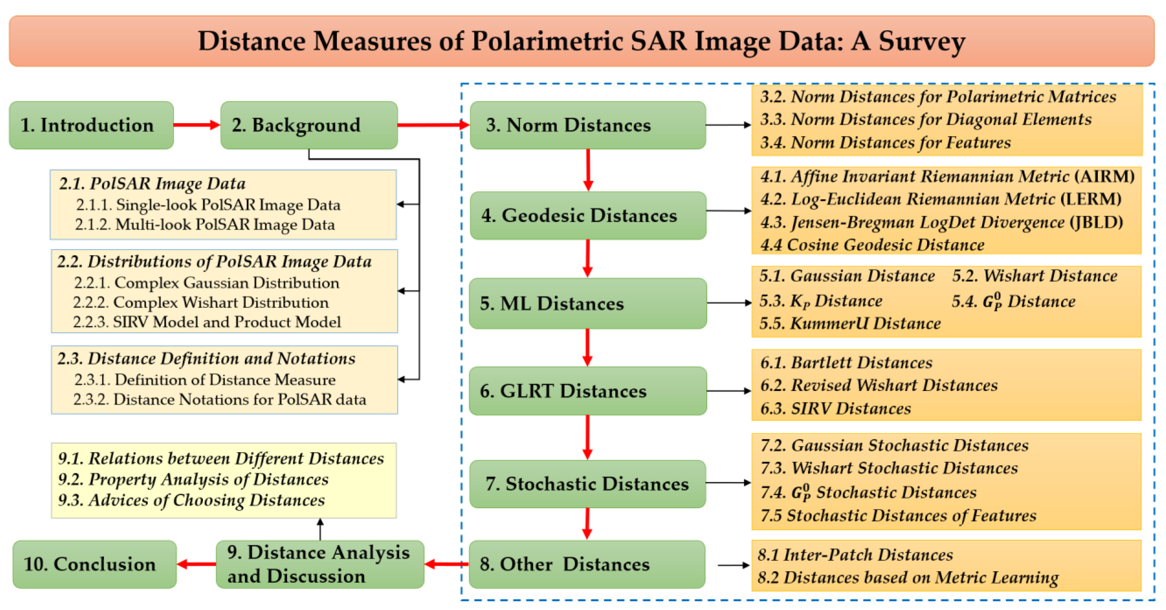
Table 1.
Notations of PolSAR image objects and distances.
| Category | Name | Notations | |
|---|---|---|---|
| Single-Look Data | Multi-Look Data | ||
| Objects | Pixels | , | |
| Pixel sets | , | , | |
| Patch pair | |||
| Class PDFs | , , | , , | |
| Distances | Inter-pixel distance | ||
| Pixel-set/class distance | , | , | |
| Inter-set/class distance | , | , | |
| Inter-patch distance | |||
Table 2.
Inter-pixel norm distances for PolSAR image data.
| Category | Name | Expression | Reference |
|---|---|---|---|
| Norm Distances for Polarimetric Matrices | Manhattan Distance | [12] | |
| Euclidean Distance | [12] | ||
| Norm Distances for Diagonal Elements | Diagonal Euclidean Distance | [48] | |
| Normalized Diagonal Euclidean Distance | [49] | ||
| Normalized Diagonal Manhattan Distance | [51] | ||
| Diagonal Revised Wishart Distance | [49] | ||
| Diagonal Relative Distance | [49] | ||
| Norm Distances for Features | Feature Euclidean Distance | [52,53,54] | |
| Weighted Feature Euclidean Distance | [55] | ||
| Modified Tensor Distance | [56] |
Table 3.
Typical ML distances for PolSAR image data.
| Name | Expression | Reference |
|---|---|---|
| Gaussian Distance | ; | [28] |
| Wishart Distance | ; | [2,11] |
| Symmetric Wishart Distance | [24] | |
| Distance | [9,14,75] | |
| Distance | [76,77] | |
| KummerU Distance | [78] |
Table 4.
Some inter-pixel GLRT distance measures for PolSAR image data.
| Name | Expression | Reference |
|---|---|---|
| Bartlett Distance | [12] | |
| Revised Wishart Distance (RWD) | [12] | |
| Symmetric RWD | [24] | |
| SIRV Distance | [32,86] | |
| Symmetric SIRV Distance | [86,87] |
Table 5.
Expressions of some typical stochastic distances.
| Name | Expression | Reference |
|---|---|---|
| KL divergence | [91] | |
| KL Distance | [91] | |
| (Original) Rényi Distance | [93] | |
| (Modified) Rényi Distance | [91] | |
| Bhattacharyya Distance | [91] | |
| Hellinger Distance | [91] | |
| Chernoff Distance | [94] | |
| JM Distance | [95] |
Table 6.
Stochastic distances between complex Wishart distributions.
| Name | Expression | Reference |
|---|---|---|
| KL Distance | [91] | |
| (Modified) Rényi Distance | [91] | |
| Bhattacharyya Distance | [91] | |
| Hellinger Distance | [91] | |
| Chernoff Distance | [94] | |
| JM Distance | [95] |
Table 7.
Properties (P1: Non-negativity, P2: Identity, P3: Symmetry, P4: Triangle inequality) and characteristics of some main distance measures of PolSAR image data. Notations “√”, “×”, and “○” denote “Yes”, “No”, and “Unknown”, respectively.
Table 7.
Properties (P1: Non-negativity, P2: Identity, P3: Symmetry, P4: Triangle inequality) and characteristics of some main distance measures of PolSAR image data. Notations “√”, “×”, and “○” denote “Yes”, “No”, and “Unknown”, respectively.
| Distance | Expression | Reference | Properties | Characteristics | ||||
|---|---|---|---|---|---|---|---|---|
| Category | Name | P1 | P2 | P3 | P4 | |||
| Norm Distances | Manhattan Distance | (16) | [12] | √ | √ | √ | √ | Defined on all elements of the data. Often leads to unsatisfactory results (possibly because their structures are quite different from the manifold of PolSAR data). |
| Euclidean Distance | (18) | [12] | √ | √ | √ | √ | ||
| Diagonal Euclidean (DE) Distance | (19) | [48] | √ | √ | √ | √ | Defined only on matrix diagonal elements; Discard some information while improving computation efficiency; The value ranges of NDE and NDM distances are and [0, 1], respectively. | |
| Normalized DE (NDE) Distance | (21) | [49] | √ | √ | √ | ○ | ||
| Normalized Diagonal Manhattan (NDM) Distance | (22) | [51] | √ | √ | √ | ○ | ||
| Diagonal Revised Wishart Distance | (26) | [49] | √ | × | √ | ○ | Simplified revised Wishart distance; The value range is [0, 4q]. | |
| Diagonal Relative Distance | (29) | [49] | √ | √ | √ | ○ | Related to the ratio of the corresponding diagonal elements. | |
| Feature Euclidean (FE) Distance | (30) | [52,53,54] | √ | √ | √ | √ | Defined on features that represent more refined PolSAR information; Often superior to the norm distances on original data. | |
| Weighted FE Distance | (31) | [55] | √ | √ | √ | √ | ||
| Modified Tensor Distance | (32) | [56] | √ | √ | √ | √ | ||
| Geodesic Distances | Affine Invariant Riemannian Metric | (34) | [60,61,62] | √ | √ | √ | ○ | Defined on the HPSD manifold of PolSAR image data or features; Requires matrix logarithm and inversion; Time-consuming. |
| Log-Euclidean Riemannian Metric | (37) | [4,62] | √ | √ | √ | ○ | Equivalent to Euclidean distance of matrices after logarithmic transformation; More efficient than AIRM. | |
| Jensen-Bregman LogDet Divergence | (39) | [59,67] | √ | √ | √ | × | Equivalent to the Bartlett distance; Simple and high-efficiency; The square root of JBLD meets the triangle inequality property [67]. | |
| Cosine Geodesic Distance | (40) | [13,72,74] | √ | √ | √ | × | Angle between the data vectors; Omit the amplitude information of data; Scale-invariant. | |
| ML Distances | Gaussian Distance | (43) | [28] | × | × | × | × | For single-look data. The earliest ML distance for PolSAR data; |
| Wishart Distance | (46) | [2,11] | × | × | × | × | For multi-look data; Widely used. | |
| Symmetric Wishart Distance | (47) | [24] | × | × | √ | × | Symmetric version of Wishart distance. | |
| Distance | (52) | [9,14,75] | × | × | × | × | Generalizations of Wishart distance; Take heterogeneous texture into account and suitable for heterogeneous PolSAR image data; Relatively complicated expression and more time-consuming. | |
| Distance | (54) | [76,77] | × | × | × | × | ||
| KummerU Distance | (57) | [78] | × | × | × | × | ||
| GLRT Distances | Bartlett Distance | (67) | [12,16] | √ | √ | √ | × | Equivalent to the JBLD for Wishart distribution. |
| Revised Wishart Distance (RWD) | (74) | [12] | √ | √ | × | × | Equivalent to the KL divergence for Wishart distribution. | |
| Symmetric RWD | (74) | [24] | √ | √ | √ | × | Equivalent to the KL distance for Wishart distribution. | |
| SIRV Distance | (80) | [32,86] | √ | × | √ | ○ | For single-look data; The NCM of each pixel is required in advance; Speckle influence is alleviated by using neighborhood data; Texture difference of data is ignored. | |
| Symmetric SIRV Distance | (81) | [86] | √ | × | √ | ○ | Symmetric version of SIRV Distance. | |
| Stochastic Distances | -KL Distance | Table 6 | [91] | √ | √ | √ | × | Equivalent to RWD when n = 1. |
| -Bhattacharyya Distance | [91] | √ | √ | √ | × | Equivalent to Bartlett distance or JBLD when n = 1. | ||
| -Hellinger Distance | [91] | √ | √ | √ | × | Can be easily transformed from Bhattacharyya distance. | ||
| -(Modifed) Rényi Distance | [91] | √ | √ | √ | × | Generalization of KL, Bhattacharyya, and Chernoff distances; An appropriate order is required in the application. | ||
| -Chernoff Distance | [94] | √ | √ | √ | × | Generalization of KL and Bhattacharyya distances; An appropriate order is required in the application. | ||
| -JM Distance | [95] | √ | √ | √ | × | Equivalent to Hellinger Distance. | ||
| -KL Distance | (90) | [93] | √ | √ | √ | × | Generalization of Wishart stochastic distances; More accurate than Wishart distance for heterogeneous data; Distribution parameters need to be estimated in advance; Complicated expressions; Calculation is time-consuming. | |
| -Rényi Distance | See [93] | [93] | √ | √ | √ | × | ||
| -Bhattacharyya Distance | [93] | √ | √ | √ | × | |||
| -Hellinger Distance | [93] | √ | √ | √ | × | |||
| JM Distance of Features | (91) | [105,106] | √ | √ | √ | × | Assume the feature vectors follow the Gaussian distribution. | |
| Discrete KL Distance of Features | (92) | [107] | √ | √ | √ | × | For each scalar feature; Replace PDFs by histograms. | |
| Inter-Patch Distances | Inter-Patch Bartlett Distance | (96) | [5,43] | √ | √ | √ | × | For multi-look data; Equal to the sum of inter-pixel Bartlett distances of all pixel pairs. |
| Inter-Patch SIRV Distance | (99) | [3] | √ | √ | √ | ○ | For single-look data; The NCM of each pixel is required in advance; Speckle influence is alleviated using neighborhood data; The contribution of texture can be added. | |
| Distances based on metric learning | Feature Mahalanobis Distance | (101) | [23] | √ | √ | √ | √ | Generalization of weighted feature Euclidean distance; Equal to Euclidean distance of the features after a linear transformation. |
| Deep metric learning Distance | Network | [118,119,120,121] | Determined by the given neural network | Use deep network to implicitly represent the distance between data; Labeled training samples are required; Network structure, loss function, and sample selection are important factors. | ||||
Publisher’s Note: MDPI stays neutral with regard to jurisdictional claims in published maps and institutional affiliations. |
© 2022 by the authors. Licensee MDPI, Basel, Switzerland. This article is an open access article distributed under the terms and conditions of the Creative Commons Attribution (CC BY) license (https://creativecommons.org/licenses/by/4.0/).
Share and Cite
MDPI and ACS Style
Qin, X.; Zhang, Y.; Li, Y.; Cheng, Y.; Yu, W.; Wang, P.; Zou, H. Distance Measures of Polarimetric SAR Image Data: A Survey. Remote Sens. 2022, 14, 5873. https://doi.org/10.3390/rs14225873
AMA Style
Qin X, Zhang Y, Li Y, Cheng Y, Yu W, Wang P, Zou H. Distance Measures of Polarimetric SAR Image Data: A Survey. Remote Sensing. 2022; 14(22):5873. https://doi.org/10.3390/rs14225873
Chicago/Turabian StyleQin, Xianxiang, Yanning Zhang, Ying Li, Yinglei Cheng, Wangsheng Yu, Peng Wang, and Huanxin Zou. 2022. "Distance Measures of Polarimetric SAR Image Data: A Survey" Remote Sensing 14, no. 22: 5873. https://doi.org/10.3390/rs14225873
Note that from the first issue of 2016, this journal uses article numbers instead of page numbers. See further details here.