Targeted Universal Adversarial Examples for Remote Sensing

Abstract

Researchers are focusing on the vulnerabilities of deep learning models for remote sensing; various attack methods have been proposed, including universal adversarial examples. Existing universal adversarial examples, however, are only designed to fool deep learning models rather than target specific goals, i.e., targeted attacks. To this end, we propose two variants of universal adversarial examples called targeted universal adversarial examples and source-targeted universal adversarial examples. Extensive experiments on three popular datasets showed strong attackability of the two targeted adversarial variants. We hope such strong attacks can inspire and motivate research on the defenses against adversarial examples in remote sensing.

1. Introduction

With the development of satellite and airborne sensors in the last few years, the amount of Earth data for observation purposes in remote sensing research has grown explosively [1], motivating and boosting many significant applications in the fields of geoscience and remote sensing [2,3]. Representative applications, including scene classification [4], object detection [5], and semantic segmentation [6] have benefited from the large amounts of quality data. Deep neural networks are widely deployed in these applications and achieve great success in interpreting these Earth observation data [7], even surpassing human performances in some tasks.

Deep neural networks, however, are found to be vulnerable to adversarial examples [8,9]. Szegedy et al. [8] discovered that with slight perturbations added to images, a well-trained classification model could output an incomprehensive prediction. Following [8], many adversarial attack methods are proposed, such as the fast gradient sign method (FGSM) [9], C&W attack [10], projected gradient descent (PGD) attack [11], and GAN-based methods [12,13]. With constraints on perturbation magnitudes, adversarial examples generated by these methods can be indistinguishable from original images in human eyes. Though imperceptible, they can be malicious and destructive to state-of-the-art deep learning models [14], leading to devastating consequences in safety–critical applications. The existence of adversarial examples would undoubtedly threaten the reliability of deep neural networks when deployed in real-world applications [11,15]. To this end, for the purpose of improving the reliability of deep learning models, the characteristics of adversarial examples should be fully explored.

In addition to the field of computer vision, there are more sensitive and safety–critical applications in remote sensing and geosciences, which are based on deep learning models. Thus, it is necessary to study adversarial examples for remote sensing. Researchers in this field recently started exploring adversarial examples for remote sensing and geoscience [16,17,18,19]. Czaja et al. [16] first revealed the existence of adversarial examples in the context of remote sensing, providing a good starting point for studying the vulnerabilities of deep learning models for remote sensing. The follow-up works further discovered adversarial examples in optical/synthetic–aperture radar (SAR) [18] and hyperspectral images [20]. In previous research on adversarial attacks in geosciences and remote sensing, white-box settings have mainly been adopted, where the attacker was assumed to access the victim model and training data when generating adversarial examples correspondingly. Xu and Ghamisi [21] argued that such an assumption is too strong to be realistic in real-world scenarios as the deployed deep neural networks are usually well-protected. In this case, it is not convenient for attackers to access models to calculate the gradients. As such, pre-calculated adversarial perturbations can be more useful for attackers. Motivated by this, Xu and Ghamisi [21] extended the research of adversarial examples for remote sensing in black-box settings, where the attacker only has limited information about the victim models, and proposed universal adversarial examples (UAE). Since such universal adversarial examples are independent of the input images, this greatly reduces the attack costs for the attackers and is more practical in real-world scenarios.

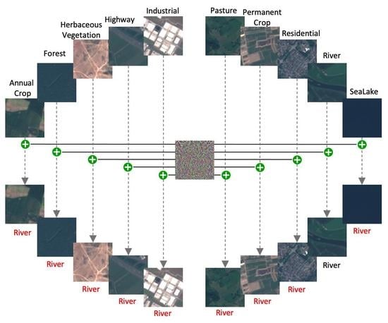
The aim of universal adversarial examples proposed by Xu and Ghamisi [21] is to fool the victim models, no matter what the final predictions are. In practice, however, attackers usually launch attacks with some specific purposes. They hope to compromise the victim models to behave as they expect; thus, the universal adversarial examples proposed by Xu and Ghamisi [21] are not suitable. On the other hand, universal adversarial perturbations are not able to reveal the vulnerabilities of victim models completely since misleading the victim models is quite basic. Studying the class-wise vulnerabilities of models might also be helpful for understanding deep learning. To this end, we propose targeted universal adversarial examples (TUAE, see Figure 1a) to fool the victim models with prefixed targets, which is evidently more challenging and promising to give us more insights into deep neural networks. Compared to universal adversarial examples, we are able to mislead the victim models with targeted universal adversarial examples to make predictions as we expect. Moreover, the attackers might only be interested in some classes for specific reasons. Targeted universal adversarial examples, however, would affect the input images from all classes, which would raise the suspicions of people [22], Thus, we further propose source-targeted universal adversarial examples (STUAE, see Figure 1b), where we compromise the victim models to misclassify the images from the source class as a different target class. In the meanwhile, the victim models would classify other images, except source classes, correctly.

The main contributions of this paper are summarized as follows.

1.

To the best of our knowledge, we are the first to study targeted universal adversarial examples in remote sensing data, without accessing the victim models in evaluation. Compared to universal adversarial examples, our research helps reveal and understand the vulnerabilities of deep learning models in remote sensing applications at a fine-grained level.

2.

We propose two variants of universal adversarial examples: targeted universal adversarial example(s) (TUAE) for all images and source-targeted universal adversarial example(s) (STUAE) for limited source images.

3.

Extensive experiments with various deep learning models on three benchmark datasets of remote sensing showed strong attackability of our methods in the scene classification task.

The rest of this paper is organized as follows. Section 2 reviews works related to this study. Section 3 elaborates on the proposed targeted universal adversarial attack methods with details. Section 4 presents the dataset information, experimental settings, implementation details, and summarizes the experimental results. Conclusions and other discussions are summarized in Section 5.

Figure 1. Illustration of our proposed TUAE (left) and STUAE (right). (a) TUAE. The target class is “forest” and images from all classes are affected by TUAE. (b) STUAE. The target class is forest and the source class is “river”. Only images from the source class are affected by STUAE.

Figure 1. Illustration of our proposed TUAE (left) and STUAE (right). (a) TUAE. The target class is “forest” and images from all classes are affected by TUAE. (b) STUAE. The target class is forest and the source class is “river”. Only images from the source class are affected by STUAE.

2. Related Work

In this section, we review the related works of adversarial attacks and universal adversarial attacks. Normally, adversarial attacks are dependent on the inputs. Universal adversarial attacks, however, do not have access to inputs and are effective. Specific methods are introduced in the following.

2.1. Adversarial Attacks

Adversarial attacks, which usually add carefully designed perturbations to the input images for fooling deep neural networks, are dependent on the input images. Correspondingly, we present the expression of adversarial perturbations below

$$\begin{array}{c}\delta =\underset{B(x,\epsilon )}{max}{\mathcal{L}}_{ce}(\theta ,x+\delta ,y),\end{array}$$

(1)

where $(x,y)\in \mathcal{D}$ represents input data randomly sampled from the dataset $\mathcal{D}$, $\theta$ concerns the parameters of the well-trained neural networks, $\epsilon$ is the maximal magnitude of perturbations, and $B(x,\epsilon )$ is the set of allowed perturbations. We express $B(x,\epsilon )$ as $B(x,\epsilon ):=\left\{x+\delta \in {\mathbb{R}}^{h\times w\times c}\mid {\parallel \delta \parallel }_p\le \epsilon \right\}$. p is used to calculate the magnitudes of perturbations, where 0, 2, and ∞ are common values of p in the literature [8,9,23].

2.1.1. Fast Gradient Sign Method (FGSM)

It is hypothesized in [9] that deep network models are sort of “linear” in high dimensional spaces. In this way, small perturbations added to input images are exaggerated when the neural networks conduct forward propagation. According to this linearity of deep neural networks, Goodfellow et al. [9] proposed the fast gradient sign method (FGSM). Specifically, FGSM first computes the gradients with respect to the inputs x but only utilizes the sign of the gradients. Adversarial perturbation $\delta$ generated by FGSM is expressed as follows:

$$\begin{array}{c}\hfill \delta =\epsilon sign\left({\nabla }_{x}J(\theta ,x,y)\right),\end{array}$$

(2)

where $\theta$ represents the parameters of the targeted classifier, $J(\theta ,x,y)$ denotes the loss function, and $ϵ$ is the magnitude of perturbations.

2.1.2. Iterative Fast Gradient Sign Method (I-FGSM)

The iterative fast gradient sign method (I-FGSM) is the iterative version of FGSM, which uses a small step size $\alpha$ and has more iterations. The generation process is formulated as

$$x^{t+1}=\mathit{Clip}\left(x^t+\alpha sign\left({\nabla }_{x}J(\theta ,x,y)\right)\right)$$

(3)

where Clip ensures the adversarial examples in a valid range.

2.1.3. C&W Attack

The C&W attack proposed by [23] is an optimization-based attack that could craft quasi-imperceptible adversarial perturbations with strong attack abilities. The objective of the C&W attack is formulated as follows:

$$minimizec·g(x+\delta )+{\parallel \delta \parallel }_{\infty }$$

(4)

with $g\left(x\right)$ defined as

$$g\left(x\right)=max\left(\underset{i\ne y}{max}\left\{f_i\left(x\right)-f_y\left(x\right)\right\},-\kappa \right)$$

(5)

where c and $\kappa (\ge 0)$ are hyperparameters, y is the true label of x, and $f_i\left(x\right)$ is the confidence of class i. The first term in Equation (4) is used to find the worst samples, while the second term is used to constrain the magnitude of the perturbations. Although C&W attacks are strong, the generation process is quite time-consuming as there exists a search for hyperparameters.

2.1.4. Projected Gradient Descent (PGD) Attack

The projected gradient descent (PGD) attack [11] is a variant of FGSM, which updates the perturbations multiple times with smaller step sizes. The PGD attack clips the adversarial examples into the neighbor $\mathcal{S}$ of the original samples after every update, defined by $ϵ$ and $l_{\infty }$. In this way, adversarial examples generated by PGD attacks are always in a valid range. The formal update scheme of the PGD attack is expressed as

$$x^{t+1}={\Pi }_{y+\mathcal{S}(x,\epsilon )}\left(x^t+\alpha sign\left({\nabla }_{x}J(\theta ,x,y)\right)\right),$$

(6)

where $\mathcal{S}(x,\epsilon ):=\left\{x+\delta \in {\mathbb{R}}^{h\times w\times c}\mid {\parallel \delta \parallel }_p\le \epsilon \right\}$ is the set of allowed perturbations to ensure the validity of $x^{t+1}$ and $\alpha$ is the step size.

2.2. Universal Attacks

The attacks mentioned in the previous subsection are all dependent on the inputs. Here, we introduce the universal attacks, which are agnostic to the inputs. Universal adversarial perturbations were first proposed in [24], which is image-agnostic and can cause natural images to be misclassified by deep neural networks. In the field of remote sensing, the very first universal adversarial examples were introduced by [21]. In their work, they proposed utilizing mix-up [25] and cut–mix [26] to enhance universal adversarial attacks. Their attacks, however, are only aimed at misleading the victim models. In other words, they are untargeted. Nevertheless, we argue that targeted universal adversarial attacks are necessary to reveal the vulnerabilities of deep neural networks. To our best knowledge, there is no prior work on targeted universal attacks in the field. Thus, we explore the targeted universal attacks and the variant class-specified targeted universal attacks to fill the gap in the literature.

3. Methodology

In this section, we present our targeted universal adversarial examples and source-targeted universal adversarial examples in detail.

3.1. Targeted Universal Adversarial Examples

3.1.1. Problem Definition

According to [21], universal adversarial examples are designed to be effective for all images and mislead the victim model f to make wrong predictions. Formally, given the dataset, e.g., $(x,y)\in \mathcal{D}$, the victim model has been trained well and has a high accuracy for classification. So, we have $f\left(x\right)=y$ in most cases. We use $x_{ua}$ to represent the corresponding adversarial counterpart of x, where $x_{ua}=x+\delta$. To generate universal adversarial examples from $\mathcal{D}$, we seek perturbation $\delta$, satisfying

$$f\left(x+\delta \right)\ne y\mathrm{subject}\mathrm{to}{\parallel \delta \parallel }_p\le ϵ,$$

(7)

where $ϵ$ is the maximal magnitude for the $l_p$ norm of the generated perturbations $\delta$, and p can be 0, 2, and ∞. We set $p=\infty$ in our paper.

Similar to universal adversarial examples, targeted universal adversarial examples are also image-agnostic. However, instead of simply fooling the victim model, we expect them to mislead the victim model to output the desired prediction class t. We use $x_{tua}$ to represent the targeted adversarial counterpart of x, where $x_{tua}=x+{\delta }_t$. Correspondingly, the perturbation ${\delta }_t$ is supposed to satisfy

$$f\left(x_{tua}\right)=t,\mathrm{subject}\mathrm{to}{\parallel {\delta }_{ct}\parallel }_p\le ϵ.$$

(8)

3.1.2. Loss Design

For classification problems, cross-entropy loss ${\mathcal{L}}_{ce}$ is the most common loss used, which is defined as

$${\mathcal{L}}_{ce}\left(f,x,y\right)=-\sum _{k=1}^{n_v}{y}^{\left(k\right)}logf{\left(x\right)}^{\left(k\right)}$$

(9)

where $n_v$ denotes the number of classes in this classification task, and y is the true class of the input samples x with one-hot encoding.

As we know, the attacker’s goal is to maximize the cross-entropy loss ${\mathcal{L}}_{ce}(f,x,y)$ for untargeted attacks and minimize the cross-entropy loss ${\mathcal{L}}_{ce}(f,x,t)$ with target class t. For targeted universal attacks, thus, we are trying to find the perturbations minimizing the targeted loss function, which is

$${\mathcal{L}}_{tu}(f,x,t,{\delta }_t)={\mathbb{E}}_{(x,y)\sim \mathcal{D}}\left[{\mathcal{L}}_{ce}(\theta ,x+{\delta }_t,t)\right].$$

(10)

Thus, our final problem to solve is

$${\delta }_t:=\underset{\parallel {\delta }_t{\parallel }_{\infty }\le ϵ}{argmin}{\mathcal{L}}_{tu}(f,x,t)$$

(11)

The training details are summarized in Algorithm 1.

Algorithm 1 Targeted universal attack.
Require: Dataset $\mathcal{D}$, Victim model f, Targeted class t, Loss function ${\mathcal{L}}_{tu}$, Number of iterations I, Perturbation magnitude $ϵ$
initialize ${\delta }_t\sim \mathcal{N}\left(0,1\right)$	▹ Random initialization
while $i<I$ do
sample $(X,Y)\in \mathcal{D}$	▹ Mini batch
$X_{adv}=X+{\delta }_t$	▹ Craft adversarial examples
$g_{{\delta }_t}=\nabla {\mathcal{L}}_{tu}(f,X,t,{\delta }_t)$	▹ Calculate gradients
${\delta }_t=Optim\left(g_{{\delta }_t}\right)$	▹ Update ${\delta }_t$
${\delta }_t=\frac{{\delta }_t}{\parallel {\delta }_t{\parallel }_p}ϵ$	▹ Projection
end while

3.2. Source-Targeted Universal Adversarial Examples

3.2.1. Problem Definition

Source-targeted universal adversarial examples are variants of targeted universal adversarial examples, where the class-specific perturbations ${\delta }_{ct}$ are only allowed to affect the images from the specified classes s and do not affect images from other classes. Note that $s\ne t$. With ${\delta }_{ct}$ added to images, we expect $f(x_s+{\delta }_{ct})=t$ while $f(x_o+{\delta }_{ct})=y_o$. Here, we use $(x_s,y_s)\in \mathcal{D}$ to denote the images from a specified class s and $(x_o,y_o)\in \mathcal{D}$ to denote the images from other classes.

Formally, the goal of the class-specific perturbation ${\delta }_{ct}$ is

$$\begin{array}{c}\hfill f\left(x_s+{\delta }_{ct}\right)=t\mathrm{while}f\left(x_o+{\delta }_{ct}\right)=y_o,\\ \hfill \mathrm{subject}\mathrm{to}\parallel {\delta }_t{\parallel }_p\le ϵ.\end{array}$$

(12)

3.2.2. Loss Design

Source-targeted universal adversarial attacks, which are different from targeted universal adversarial attacks targeting all of the images, are only for the specified classes and have no or little effects on other classes. Source-targeted universal adversarial attacks are two-fold. First, with the class-specific perturbations ${\delta }_{ct}$, images from class s would be predicted by the victim model f as the target class t. Second, images from other classes with ${\delta }_{ct}$ can be classified correctly by f. Thus, the overall loss source-targeted universal adversarial attacks ${\mathcal{L}}_{st}$ consists of two parts: the loss for class s—${\mathcal{L}}_s$ and the loss for other classes —${\mathcal{L}}_{other}$.

Specifically, ${\mathcal{L}}_s$ is defined as

$${\mathcal{L}}_s(f,x_s,t,{\delta }_{ct})={\mathbb{E}}_{(x_s,y_s)\sim \mathcal{D}}\left[{\mathcal{L}}_{ce}(\theta ,x_s+{\delta }_{ct},t)\right].$$

(13)

The loss ${\mathcal{L}}_{other}$ involves maintaining the performance of the victim model f on images from other classes when added ${\delta }_{ct}$. Thus, we have ${\mathcal{L}}_{other}$ expressed as

$${\mathcal{L}}_{other}(f,x_o,y_o,{\delta }_{ct})={\mathbb{E}}_{(x_o,y_o)\sim \mathcal{D}}\left[{\mathcal{L}}_{ce}(\theta ,x_o+{\delta }_{ct},y_o)\right].$$

(14)

Considering that f can never be perfect to classify all images correctly, we instead replace the true label $y_o$ with the victim model’s predictions $f\left(x_o\right)$ in ${\mathcal{L}}_{other}$. Thus, the new ${\mathcal{L}}_{other}$ is rewritten as

$${\mathcal{L}}_{other}(f,x_o,{\delta }_{ct})={\mathbb{E}}_{(x_o,y_o)\sim \mathcal{D}}\left[{\mathcal{L}}_{ce}(\theta ,x_o+{\delta }_{ct},max\left(f\left(x_o\right)\right))\right].$$

(15)

Then we have ${\mathcal{L}}_{st}$ as the sum of ${\mathcal{L}}_s$ and ${\mathcal{L}}_{other}$,

$${\mathcal{L}}_{st}={\mathcal{L}}_s+\alpha \times {\mathcal{L}}_{other},$$

(16)

where $\alpha$ is a hyperparameter for balancing these two losses. The training details are summarized in Algorithm 2.

Algorithm 2 Source-targeted universal attack.
Require: Dataset $\mathcal{D}$, Victim model f, Specified class s, Targeted class t, Loss function ${\mathcal{L}}_{tu}$, Number of iterations I, Perturbation magnitude $ϵ$, hyperparameter $\alpha$
initialize ${\delta }_{ct}\sim \mathcal{N}\left(0,1\right)$	▹Random initialization
while $i<I$ do
sample $(X,Y)\in \mathcal{D}$	▹ Mini batch
$X_{adv}=X+{\delta }_{ct}$	▹ Craft adversarial examples
$M=\left\{1\right|Y=s\}$	▹ Generate mask
$X_s=X·M$	▹ Select specified class samples
$X_o=X·(1-M),Y_o=Y·(1-M)$	▹ Select other class samples
${\mathcal{L}}_{st}={\mathcal{L}}_s(f,X_s,t,{\delta }_{ct})+\alpha \times {\mathcal{L}}_{other}(f,X_o,Y_o,{\delta }_{ct})$	▹ Calculate loss
$g_{{\delta }_t}=\nabla {\mathcal{L}}_{st}(f,X_s,X_o,Y_o,t,{\delta }_{ct})$	▹ Calculate gradients
${\delta }_{ct}=Optim\left(g_{{\delta }_{ct}}\right)$	▹ Update ${\delta }_{ct}$
${\delta }_{ct}=\frac{{\delta }_{ct}}{\parallel {\delta }_{ct}{\parallel }_p}ϵ$	▹ Projection
end while

4. Experiments

In this section, we first introduce three datasets and experimental settings, then report and discuss the results of our two proposed attacks.

4.1. Data Descriptions

We utilized three remote sensing image datasets for scene classification: UCM (http://weegee.vision.ucmerced.edu/datasets/landuse.html (accessed on 1 September 2022)) (UC Merced Land Use Dataset), AID (Aerial Image Dataset) (https://captain-whu.github.io/AID/ (accessed on 1 September 2022)) and EuroSAT [27]. The details of the three datasets are elaborated as follows.

UCM: There are 2100 overhead scene images with 21 land use classes in UCM. For each class, there are 100 aerial images, 256 × 256, which are extracted from large images from the USGS National Map Urban Area Imagery collection for various urban areas around the country. The 21 land-use classes are agricultural, airplane, baseball diamond, beach, buildings, chaparral, dense residential, forest, freeway, golf course, harbor, intersection, medium residential, mobile home park, overpass, parking lot, river, runway, sparse residential, storage tanks, and tennis court.

AID: AID is a large-scale aerial image dataset collected from Google Earth imagery. AID consists of the following 30 aerial scene types: airport, bare land, baseball field, beach, bridge, center, church, commercial, dense residential, desert, farmland, forest, industrial, meadow, medium residential, mountain, park, parking, playground, pond, port, railway station, resort, river, school, sparse residential, square, stadium, storage tanks, and viaduct. There are 10,000 images in total in AID, and the image numbers for each class are not identical, varying from 220 to 420. The pixel size of each image is 600 × 600 pixels.

EuroSAT: EuroSAT is a satellite image dataset for land use and land cover classification tasks, created from satellite images taken by the satellite Sentinel-2A via Amazon S3; it covers over 34 European countries. It consists of 27,000 labeled images measuring 64 × 64 pixels with 10 different classes: AnnualCrop, Forest, HerbaceousVegatation, Highway, Industrial, Pasture, PermanentCrop, Residential, River, and SeaLake.

4.2. Experimental Settings and Implementation Details

In comparison with our method, we selected several popular adversarial attacks: FGSM [9], I-FGSM [28], C&W [23], and PGD [11] to conduct the targeted adversarial attacks for scene classifications on UCM, AID, and EuroSAT, respectively. For every dataset, we evaluated the above attacks on several different well-trained victim models with various architectures: AlexNet [29], ResNet18 [30], DenseNet121 [31], and RegNetX-400MF [32]. Following the setting in [21], we set the number of total iterations to 5 for iterative attacks, such as I-FGSM, C&W, and PGD. The magnitude of perturbations was set to $l_{\infty }\left(ϵ\right)=15$ for images in the range [0, 255]. The implementations of FGSM, I-FGSM, C&W, and PGD were from [33] (https://github.com/Harry24k/adversarial-attacks-pytorch (accessed on 25 September 2022)).

For our two universal attacks in the following experiments, the number of iterations was set to I = 500. We used statistical gradient descent (SGD) with momentum to optimize the perturbations. The target classes and source classes were randomly sampled.

All our experiments were implemented by PyTorch [34] and ran on a single NVIDIA GPU A100.

4.3. Attacks on Scene Classification

4.3.1. Targeted Adversarial Attacks

In this section, we mainly compare the various targeted attacks: FGSM, I-FGSM, TPGD, and C&W with our TUAE. For a fair comparison, we made necessary modifications to these four attack methods to the targeted attacks. Take FGSM as an example, the perturbations for targeted attacks are defined as

$$\begin{array}{c}\hfill \delta =-\epsilon sign(\nabla J_x(\theta ,x,t)),\end{array}$$

(17)

where $J(\theta ,x,t)$ denotes the loss functions for a targeted attack, and $ϵ$ is the magnitude of the perturbation.

To show the effectiveness of TUAE for each target class, we mainly conducted experiments on the EuroSAT dataset. Specifically, we attacked 4 victim models with 10 different targets (10 classes in EuroSAT) to show the effectiveness of TUAE. The experimental results are summarized in

Table 1. Targeted attack success rate(s) (TSR) of various attacks (FGSM, I-FGSM, PGD, C&W, and our TUAE) on EuroSAT data. TSR is defined as $\frac{\# \mathrm{of} \mathrm{test} \mathrm{samples} \mathrm{predicted} \mathrm{to} \mathrm{Class} \mathrm{t}}{\# \mathrm{of} \mathrm{all} \mathrm{test} \mathrm{samples}}$. The higher, the better. The highest TSR in every row is in bold text.

Model	Target Class	FGSM	I-FGSM	C&W	PGD	TUAE
AlexNet	0	0.00%	99.67%	39.48%	99.69%	99.48%
	1	0.02%	76.85%	23.94%	82.11%	99.52%
	2	0.00%	97.91%	35.76%	98.57%	99.80%
	3	0.54%	100.00%	49.06%	99.96%	99.91%
	4	1.87%	94.04%	16.94%	98.54%	99.94%
	5	0.00%	98.57%	30.50%	98.61%	99.78%
	6	0.00%	99.81%	51.81%	99.69%	99.54%
	7	99.85%	100.00%	23.17%	100.00%	100.00%
	8	0.00%	99.96%	41.61%	99.93%	97.54%
	9	0.00%	92.57%	22.94%	91.19%	99.26%
DenseNet121	0	0.26%	99.96%	50.94%	100.00%	100.00%
	1	0.00%	95.93%	47.11%	99.19%	100.00%
	2	0.00%	98.24%	56.33%	96.07%	100.00%
	3	0.00%	99.93%	47.33%	100.00%	100.00%
	4	0.46%	100.00%	35.22%	100.00%	100.00%
	5	0.00%	100.00%	54.63%	100.00%	100.00%
	6	0.02%	100.00%	80.94%	100.00%	100.00%
	7	99.93%	100.00%	61.87%	100.00%	100.00%
	8	0.00%	99.78%	35.37%	99.87%	100.00%
	9	0.09%	100.00%	34.69%	100.00%	100.00%
RegNet_x_400mf	0	33.69%	100.00%	55.22%	100.00%	100.00%
	1	0.00%	84.93%	11.43%	95.85%	99.98%
	2	0.00%	93.63%	25.56%	95.93%	99.98%
	3	0.00%	99.67%	33.61%	99.57%	99.98%
	4	0.00%	99.94%	30.87%	99.98%	100.00%
	5	0.00%	100.00%	29.76%	99.98%	100.00%
	6	0.00%	99.98%	69.63%	99.98%	100.00%
	7	0.00%	100.00%	67.69%	100.00%	100.00%
	8	0.00%	100.00%	32.15%	100.00%	100.00%
	9	66.76%	100.00%	34.65%	100.00%	100.00%
ResNet18	0	0.06%	96.65%	41.46%	98.85%	100.00%
	1	7.76%	99.98%	51.94%	100.00%	99.94%
	2	0.00%	99.96%	50.52%	99.96%	99.89%
	3	2.46%	99.81%	48.17%	99.98%	100.00%
	4	5.11%	100.00%	34.48%	100.00%	99.98%
	5	0.00%	99.89%	42.33%	99.65%	99.98%
	6	0.00%	99.93%	61.31%	99.91%	99.94%
	7	93.74%	100.00%	57.24%	100.00%	100.00%
	8	0.22%	99.98%	41.65%	99.98%	100.00%
	9	0.02%	99.91%	20.48%	99.98%	99.69%

. The targeted attack success rate (TSR) is defined as $\frac{\# \mathrm{of} \mathrm{test} \mathrm{samples} \mathrm{predicted} \mathrm{to} \mathrm{Class} \mathrm{t}}{\# \mathrm{of} \mathrm{all} \mathrm{test} \mathrm{samples}}$. The higher TSR, the stronger the attacks.

As shown in Table 1, our TUAE can achieve comparable TSR to the other four popular methods, but our method is universal and does not have to access images when testing. This makes it applicable in practice for black-box attacks. Adversarial examples generated by these attacks are shown in Figure 2.

4.3.2. Source-Targeted Universal Adversarial Examples

We now evaluate and report on the experimental results of our source-targeted universal adversarial example(s) (STUAE). Different from TUAE, we assigned source classes and target classes in STUAE. The goal of STUAE is to craft universal adversarial perturbations for images from the source class to be predicted as the target classes while maintaining benign the images from other classes. Thus, there were two evaluation metrics for STUAE: we used source rate (SR, the higher, the better) to denote the TSR for source images and other rates (OR, the lower, the better) to denote the TSR for other class images. We conducted experiments with four different models: AlexNet, DenseNet121, RegNet_x_400mf, and ResNet18 on three datasets: EuroSAT, AID, and UCM. The respective experimental results are summarized in

Table 2. TSR of STUAE on EuroSAT with four victim models: AlexNet, DenseNet121, RegNet_x_400mf, and ResNet18. The goal of the adversaries is to mislead victim models to recognize images from the source class to the target class. SR (the higher, the better) stands for the ratio of images from the source class to be predicted as the target class, while OR (the lower, the better) stands for the ratio of images from the other classes to be predicted as the target class.

Target Class	Source Class	Victim Model
		AlexNet		DenseNet121		RegNet_x_400mf		ResNet18
		SR	OR	SR	OR	SR	OR	SR	OR
5	9	96.33%	12.38%	98.67%	12.35%	96.00%	12.56%	95.00%	12.71%
6	9	83.83%	12.38%	96.17%	12.38%	94.00%	12.56%	97.33%	12.69%
4	9	87.00%	12.02%	94.20%	12.10%	89.40%	12.31%	96.40%	12.47%
3	4	98.20%	12.14%	98.40%	12.12%	100.00%	12.31%	99.40%	12.47%
0	9	97.50%	11.84%	99.25%	11.82%	93.75%	11.94%	98.75%	12.20%
4	7	93.80%	12.02%	97.80%	12.04%	87.80%	12.08%	97.80%	12.27%
8	9	95.50%	12.40%	97.67%	12.38%	99.83%	12.56%	99.67%	12.73%
6	1	92.40%	12.08%	94.00%	12.12%	96.80%	12.31%	98.20%	12.43%
3	7	97.17%	12.35%	99.67%	12.35%	98.83%	12.56%	99.83%	12.69%
7	4	94.67%	11.00%	97.00%	12.40%	95.33%	12.52%	98.50%	12.46%

,

Table 3. TSR of STUAE on AID with four victim models: AlexNet, DenseNet121, RegNet_x_400mf, and ResNet18. The goal of the adversaries is to mislead victim models to recognize images from source class to the target class. SR (the higher, the better) stands for the ratio of images from the source class to be predicted as the target class, while OR (the lower, the better) stands for the ratio of images from the other classes to be predicted as the target class.

Target Class	Source Class	Victim Model
		AlexNet		DenseNet121		RegNet_x_400mf		ResNet18
		SR	OR	SR	OR	SR	OR	SR	OR
0	1	89.68%	3.61%	90.97%	3.80%	81.29%	3.78%	94.19%	3.82%
8	11	72.80%	4.64%	71.20%	4.23%	72.80%	4.74%	67.20%	3.63%
9	1	90.97%	2.97%	94.19%	3.01%	94.84%	3.03%	97.42%	2.95%
11	9	88.00%	2.74%	92.67%	2.56%	94.00%	2.58%	99.33%	2.78%
13	10	82.16%	2.91%	80.54%	2.95%	80.00%	2.91%	79.46%	2.97%
14	13	94.29%	2.96%	93.57%	3.13%	97.86%	3.13%	92.86%	2.82%
15	13	97.14%	3.58%	93.57%	3.50%	100.00%	3.46%	97.14%	3.46%
16	18	84.87%	3.88%	88.11%	3.55%	91.89%	3.78%	94.05%	4.36%
17	13	91.43%	3.93%	92.86%	4.01%	97.86%	4.01%	97.86%	3.89%
19	3	90.00%	4.33%	89.50%	4.52%	81.00%	4.40%	92.00%	4.42%

and

Table 4. TSR of STUAE on UCM with four victim models: AlexNet, DenseNet121, RegNet_x_400mf, and ResNet18. The goal of adversaries is to mislead victim models to recognize images from the source class to the target class. SR (the higher, the better) stands for the ratio of images from the source class to be predicted as the target class, while OR (the lower, the better) stands for the ratio of images from the other classes to be predicted as the target class.

Target Class	Source Class	Victim Model
		AlexNet		DenseNet121		RegNet_x_400mf		ResNet18
		SR	OR	SR	OR	SR	OR	SR	OR
9	3	96.00%	6.60%	98.00%	7.70%	100.00%	7.20%	100.00%	7.70%
0	3	90.00%	6.70%	98.00%	6.70%	92.00%	6.20%	100.00%	7.10%
2	3	86.00%	7.10%	100.00%	7.40%	98.00%	11.20%	98.00%	8.90%
1	3	78.00%	7.80%	100.00%	7.90%	94.00%	9.10%	98.00%	6.60%
7	16	70.00%	8.80%	78.00%	8.50%	80.00%	8.90%	70.00%	10.10%
7	5	92.00%	6.30%	42.00%	6.10%	78.00%	7.80%	70.00%	9.90%
18	9	70.00%	10.50%	66.00%	9.40%	82.00%	11.30%	72.00%	9.60%
20	2	80.00%	13.50%	62.00%	7.20%	54.00%	7.30%	76.00%	11.60%
16	17	56.00%	8.60%	54.00%	9.80%	64.00%	7.90%	54.00%	9.30%
20	9	52.00%	16.30%	54.00%	8.10%	64.00%	10.00%	68.00%	12.90%

.

For each dataset, we sampled ten (source, target) pairs to demonstrate the effectiveness of our method. With extensive experiments, we can see that in most cases, our STUAE can produce strong attacks (high SR) for source class images and benign (low OR) for target class images. For some scenarios, such as the last row in Table 4, it is not as effective as others. We assume this is due to the robust samples in a dataset, which are not easy to attack. Overall, it is safe to conclude several advantages of STUAE: (1) STUAE can be used as easily as UAE [21] since both attacks do not require access to the victim models and save the computation costs; (2) Compared to UAE, STUAE is more advanced and achieves a more complicated goal, which targets a specific class. To this end, STUAE is more difficult to be detected. Samples for each dataset are shown in Figure 3, Figure 4 and Figure 5, respectively.

We further study the necessities of ${\mathcal{L}}_{other}$ in ${\mathcal{L}}_{st}$. Specifically, we set $\alpha =0$ in ${\mathcal{L}}_{st}$ and test STUAE on EuroSAT; the evaluation results can be found in

Table 5. Comparisons of TSR of STUAE on EuroSAT when $alpha=0$ and $alpha=1$.

Target Class	Source Class	Victim Model
		AlexNet		DenseNet121		RegNet_x_400mf		ResNet18
		$\alpha =\mathbf{1}$	$\alpha =\mathbf{0}$	$\alpha =\mathbf{1}$	$\alpha =\mathbf{0}$	$\alpha =\mathbf{1}$	$\alpha =\mathbf{0}$	$\alpha =\mathbf{1}$	$\alpha =\mathbf{0}$
5	9	12.38%	61.60%	12.35%	65.06%	12.56%	98.23%	12.71%	71.50%
6	9	12.38%	69.04%	12.38%	78.35%	12.56%	99.15%	12.69%	85.65%
4	9	12.02%	88.56%	12.10%	91.27%	12.31%	100.00%	12.47%	99.88%
3	4	12.14%	99.98%	12.12%	100.00%	12.31%	99.98%	12.47%	100.00%
0	9	11.84%	66.58%	11.82%	69.88%	11.94%	99.88%	12.20%	69.04%
4	7	12.02%	99.50%	12.04%	100.00%	12.08%	99.75%	12.27%	100.00%
8	9	12.40%	63.48%	12.38%	59.75%	12.56%	89.02%	12.73%	93.40%
6	1	12.08%	76.10%	12.12%	87.25%	12.31%	96.06%	12.43%	93.60%
3	7	12.35%	99.77%	12.35%	100.00%	12.56%	99.50%	12.69%	99.96%
7	4	11.00%	100.00%	12.40%	100.00%	12.52%	100.00%	12.46%	100.00%

. As indicated in Table 5, the universal perturbations generated on only source class images would have substantial effects on the images of other classes. Thus, it is critical to limit the influences of universal perturbations during the generation process. For this reason, we chose $\alpha =1$ in our experiments; it is common to give the same weights when there are multiple terms of loss functions. In our case, we found the experimental results with this default setting to be satisfactory.

5. Conclusions

In this paper, we studied the universal adversarial examples in the field of remote sensing and proposed two variant universal adversarial examples: TUAE and STUAE. These two kinds of universal adversarial examples both achieve high attack success rates in the targeted attack scenario. We hope our two kinds of UAE can be helpful in discovering the vulnerabilities of deep learning models for remote sensing. On the other hand, there are some issues we have not explored: (1) We mainly focused on the white-box settings. The transferability of targeted universal adversarial examples was not studied in this paper. (2) Our experiments show that we can generate strong UAE with images from a single class. This inspires us to consider how to generate UAE with few samples, which has rarely been studied for UAE and reduces the training cost greatly. We hope to solve the above two issues in future works.

References

- Boukabara, S.A.; Eyre, J.; Anthes, R.A.; Holmlund, K.; Germain, K.M.S.; Hoffman, R.N. The Earth-Observing Satellite Constellation: A review from a meteorological perspective of a complex, interconnected global system with extensive applications. IEEE Geosci. Remote Sens. Mag. 2021, 9, 26–42. [Google Scholar] [CrossRef]
- Xu, Y.; Du, B.; Zhang, L.; Cerra, D.; Pato, M.; Carmona, E.; Prasad, S.; Yokoya, N.; Hänsch, R.; Le Saux, B. Advanced multi-sensor optical remote sensing for urban land use and land cover classification: Outcome of the 2018 IEEE GRSS data fusion contest. IEEE J. Sel. Top. Appl. Earth Obs. Remote Sens. 2019, 12, 1709–1724. [Google Scholar] [CrossRef]
- Ghamisi, P.; Rasti, B.; Yokoya, N.; Wang, Q.; Hofle, B.; Bruzzone, L.; Bovolo, F.; Chi, M.; Anders, K.; Gloaguen, R.; et al. Multisource and multitemporal data fusion in remote sensing: A comprehensive review of the state of the art. IEEE Geosci. Remote Sens. Mag. 2019, 7, 6–39. [Google Scholar] [CrossRef] [Green Version]
- Cheng, G.; Han, J.; Lu, X. Remote sensing image scene classification: Benchmark and state of the art. Proc. IEEE 2017, 105, 1865–1883. [Google Scholar] [CrossRef] [Green Version]
- Wu, X.; Li, W.; Hong, D.; Tao, R.; Du, Q. Deep learning for unmanned aerial vehicle-based object detection and tracking: A survey. IEEE Geosci. Remote Sens. Mag. 2021, 10, 91–124. [Google Scholar] [CrossRef]
- Ghorbanzadeh, O.; Tiede, D.; Wendt, L.; Sudmanns, M.; Lang, S. Transferable instance segmentation of dwellings in a refugee camp-integrating CNN and OBIA. Eur. J. Remote Sens. 2021, 54, 127–140. [Google Scholar] [CrossRef]
- Zhang, L.; Zhang, L.; Du, B. Deep learning for remote sensing data: A technical tutorial on the state of the art. IEEE Geosci. Remote Sens. Mag. 2016, 4, 22–40. [Google Scholar] [CrossRef]
- Szegedy, C.; Zaremba, W.; Sutskever, I.; Bruna, J.; Erhan, D.; Goodfellow, I.J.; Fergus, R. Intriguing properties of neural networks. Conference Track Proceedings. In Proceedings of the 2nd International Conference on Learning Representations, ICLR 2014, Banff, AB, Canada, 14–16 April 2014. [Google Scholar]
- Goodfellow, I.J.; Shlens, J.; Szegedy, C. Explaining and Harnessing Adversarial Examples. In Proceedings of the ICLR, San Diego, CA, USA, 7–9 May 2015. [Google Scholar]
- Carlini, N.; Wagner, D. Towards Evaluating the Robustness of Neural Networks. In Proceedings of the 2017 IEEE Symposium on Security and Privacy (SP), San Jose, CA, USA, 22–26 May 2017. [Google Scholar]
- Madry, A.; Makelov, A.; Schmidt, L.; Tsipras, D.; Vladu, A. Towards Deep Learning Models Resistant to Adversarial Attacks. Conference Track Proceedings. In Proceedings of the 6th International Conference on Learning Representations, ICLR 2018, Vancouver, BC, Canada, 30 April–3 May 2018. [Google Scholar]
- Xiao, C.; Li, B.; Zhu, J.; He, W.; Liu, M.; Song, D. Generating Adversarial Examples with Adversarial Networks. In Proceedings of the Twenty-Seventh International Joint Conference on Artificial Intelligence, IJCAI 2018, Stockholm, Sweden, 13–19 July 2018. [Google Scholar]
- Bai, T.; Zhao, J.; Zhu, J.; Han, S.; Chen, J.; Li, B.; Kot, A. AI-GAN: Attack-Inspired Generation of Adversarial Examples. In Proceedings of the 2021 IEEE International Conference on Image Processing (ICIP), Anchorage, AL, USA, 19–22 September 2021; pp. 2543–2547. [Google Scholar] [CrossRef]
- Akhtar, N.; Mian, A. Threat of Adversarial Attacks on Deep Learning in Computer Vision: A Survey. arXiv 2018, arXiv:1801.00553. [Google Scholar] [CrossRef]
- Kurakin, A.; Goodfellow, I.J.; Bengio, S. Adversarial Machine Learning at Scale. Conference Track Proceedings. In Proceedings of the 5th International Conference on Learning Representations, ICLR 2017, Toulon, France, 24–26 April 2017. [Google Scholar]
- Czaja, W.; Fendley, N.; Pekala, M.; Ratto, C.; Wang, I.J. Adversarial examples in remote sensing. In Proceedings of the 26th ACM SIGSPATIAL International Conference on Advances in Geographic Information Systems, Washington, DC, USA, 6–9 November 2018; pp. 408–411. [Google Scholar]
- Xu, Y.; Du, B.; Zhang, L. Assessing the threat of adversarial examples on deep neural networks for remote sensing scene classification: Attacks and defenses. IEEE Trans. Geosci. Remote Sens. 2020, 59, 1604–1617. [Google Scholar] [CrossRef]
- Chen, L.; Zhu, G.; Li, Q.; Li, H. Adversarial example in remote sensing image recognition. arXiv 2019, arXiv:1910.13222. [Google Scholar]
- Chan-Hon-Tong, A.; Lenczner, G.; Plyer, A. Demotivate adversarial defense in remote sensing. In Proceedings of the 2021 IEEE International Geoscience and Remote Sensing Symposium IGARSS, Brussels, Belgium, 11–16 July 2021; pp. 3448–3451. [Google Scholar]
- Xu, Y.; Du, B.; Zhang, L. Self-attention context network: Addressing the threat of adversarial attacks for hyperspectral image classification. IEEE Trans. Image Process. 2021, 30, 8671–8685. [Google Scholar] [CrossRef] [PubMed]
- Xu, Y.; Ghamisi, P. Universal Adversarial Examples in Remote Sensing: Methodology and Benchmark. IEEE Trans. Geosci. Remote Sens. 2022, 60, 1–15. [Google Scholar] [CrossRef]
- Benz, P.; Zhang, C.; Imtiaz, T.; Kweon, I.S. Double targeted universal adversarial perturbations. In Proceedings of the Asian Conference on Computer Vision, Kyoto, Japan, 30 November–4 December 2020. [Google Scholar]
- Carlini, N.; Athalye, A.; Papernot, N.; Brendel, W.; Rauber, J.; Tsipras, D.; Goodfellow, I.; Madry, A.; Kurakin, A. On Evaluating Adversarial Robustness. arXiv 2019, arXiv:1902.06705. [Google Scholar]
- Moosavi-Dezfooli, S.M.; Fawzi, A.; Fawzi, O.; Frossard, P. Universal adversarial perturbations. In Proceedings of the IEEE Conference on Computer Vision and Pattern Recognition, Honolulu, HI, USA, 21–26 July 2017; pp. 1765–1773. [Google Scholar]
- Zhang, H.; Cisse, M.; Dauphin, Y.N.; Lopez-Paz, D. mixup: Beyond empirical risk minimization. arXiv 2017, arXiv:1710.09412. [Google Scholar]
- Yun, S.; Han, D.; Oh, S.J.; Chun, S.; Choe, J.; Yoo, Y. Cutmix: Regularization strategy to train strong classifiers with localizable features. In Proceedings of the IEEE/CVF International Conference on Computer Vision, Seoul, Korea, 27 October–2 November 2019; pp. 6023–6032. [Google Scholar]
- Helber, P.; Bischke, B.; Dengel, A.; Borth, D. Eurosat: A novel dataset and deep learning benchmark for land use and land cover classification. IEEE J. Sel. Top. Appl. Earth Obs. Remote Sens. 2019, 14, 1–9. [Google Scholar] [CrossRef] [Green Version]
- Kurakin, A.; Goodfellow, I.; Bengio, S. Adversarial machine learning at scale. arXiv 2016, arXiv:1611.01236. [Google Scholar]
- Krizhevsky, A.; Sutskever, I.; Hinton, G.E. Imagenet classification with deep convolutional neural networks. Commun. ACM 2017, 60, 84–90. [Google Scholar] [CrossRef] [Green Version]
- He, K.; Zhang, X.; Ren, S.; Sun, J. Deep residual learning for image recognition. In Proceedings of the IEEE Conference on Computer Vision and Pattern Recognition, Las Vegas, NV, USA, 27–30 June 2016; pp. 770–778. [Google Scholar]
- Huang, G.; Liu, Z.; Van Der Maaten, L.; Weinberger, K.Q. Densely connected convolutional networks. In Proceedings of the IEEE Conference on Computer Vision and Pattern Recognition, Honolulu, HI, USA, 21–26 July 2017; pp. 4700–4708. [Google Scholar]
- Radosavovic, I.; Kosaraju, R.P.; Girshick, R.; He, K.; Dollár, P. Designing network design spaces. In Proceedings of the IEEE/CVF Conference on Computer Vision and Pattern Recognition, Seattle, WA, USA, 14–19 June 2020; pp. 10428–10436. [Google Scholar]
- Kim, H. Torchattacks: A pytorch repository for adversarial attacks. arXiv 2020, arXiv:2010.01950. [Google Scholar]
- Paszke, A.; Gross, S.; Massa, F.; Lerer, A.; Bradbury, J.; Chanan, G.; Killeen, T.; Lin, Z.; Gimelshein, N.; Antiga, L.; et al. PyTorch: An Imperative Style, High-Performance Deep Learning Library. In Advances in Neural Information Processing Systems 32; Wallach, H., Larochelle, H., Beygelzimer, A., d’Alché-Buc, F., Fox, E., Garnett, R., Eds.; Curran Associates Inc.: Red Hook, NY, USA, 2019; pp. 8024–8035. [Google Scholar]
Figure 2.
Targeted adversarial samples generated by various attacks. Numbers on the left side are targeted classes when generating adversarial examples. Here, we used AlexNet as the victim model for visualization.
Figure 3.
Samples of source-targeted universal adversarial examples on EuroSAT. The upper row shows the images from source classes, while the lower row shows the corresponding targeted adversarial examples, misleading the victim models to predict the target classes.
Figure 4.
Samples of source-targeted universal adversarial examples on AID. The upper row shows the images from source classes, while the lower row shows the corresponding targeted adversarial examples, misleading the victim models to predict the target classes.
Figure 5.
Samples of Source-Targeted Universal Adversarial Examples on UCM. The upper row shows the images from source classes, while the lower row shows the corresponding targeted adversarial examples, misleading the victim models to predict the target classes.